Embedded discontinuous Galerkin transport schemes with localised limiters

C. J. Cotter Department of Mathematics, Imperial College London, South Kensington Campus, London SW7 2AZ D. Kuzmin Institute of Applied Mathematics, Dortmund University of Technology, Vogelpothsweg 87, D-44227 Dortmund, Germany
(P2; vertical; Recently there has been a lot of activity in the development of finite element methods for numerical weather prediction (NWP), using continuous (mainly spectral) finite elements as well as discontinuous finite elements (Fournier et al., 2004; Thomas and Loft, 2005; Dennis et al., 2011; Kelly and Giraldo, 2012; Giraldo et al., 2013; Marras et al., 2013; Brdar et al., 2013; Bao et al., 2015); see Marras et al. (2015) for a comprehensive review. A key aspect of NWP models is the need for transport schemes that preserve discrete analogues of properties of the transport equation such as monotonicity (shape preservation) and positivity; these properties are particularly important when treating tracers such as moisture. Discontinuous Galerkin methods can be interpreted as a generalisation of finite volume methods and hence the roadmap for the development of shape preserving and positivity preserving methods is relatively clear (see Cockburn and Shu (2001) for an introduction to this topic). However, this is not the case for continuous Galerkin methods, and so different approaches must be used. In the NWP community, limiters for CG methods have been considered by Marras et al. (2012), who used first-order subcells to reduce the method to first-order upwind in oscillatory regions, and Guba et al. (2014), who exploited the monotonicity of the element-averaged scheme in the spectral element method to build a quasi-monotone limiter. ; In this paper, we address the problem of finding suitable limiters for the partially continuous finite element spaces for tracers that arise in the framework of compatible finite element methods for numerical weather prediction models (Cotter and Shipton, 2012; Cotter and Thuburn, 2014; Staniforth et al., 2013; McRae and Cotter, 2014). Compatible finite element methods have been proposed as an evolution of the C-grid staggered finite difference methods that are very popular in NWP.; Within the UK dynamical core “Gung-Ho” project; evolution; (Staniforth and Thuburn, 2012); Compatible finite element; (Biswas et al., 1994; Burbeau et al., 2001; Cockburn and Shu, 2001; Hoteit et al., 2004; Krivodonova et al., 2004; Tu and Aliabadi, 2005; Kuzmin, 2010; Zhang and Shu, 2011); The main results of this paper are:
  1. 1.

    The introduction of an embedded discontinuous Galerkin scheme which is demonstrated to be linearly stable,

  2. 2.

    The introduction of localised element-based limiters to remove spurious oscillations when projecting from from discontinuous to continuous finite element spaces, which are necessary to make the whole transport scheme bounded,

  3. 3.

    When combined with standard limiters for the discontinuous Galerkin stage, the overall scheme remains locally bounded, addressing the previously unsolved problem of how to limit partially continuous finite element spaces that arise in the compatible finite element framework.

Our bounded transport scheme can also be used for continuous finite element methods, although other approaches are available that do not involve intermediate use of discontinuous Galerkin methods.; Figure Embedded discontinuous Galerkin transport schemes with localised limiters provides diagrams showing the nodes for these spaces in the case $k=1$.;
Figure 1: Diagrams showing the nodes for the various spaces in the compatible finite element framework in the 2D vertical slice case and degree $k=1$. From left to right: the velocity space $RT_{1}$, the pressure space $DG_{1}\times DG_{1}$, the vertical part of the velocity space $RT_{1}$, and the temperature space $DG_{1}\times CG_{2}$. Circles denote scalar nodes, whilst lines denote normal components of a vector.
;
Figure 2: Diagrams showing the nodes for the partially continuous space $V$ and the discontinuous space $\hat{V}$, in the case $V=DG_{1}\times CG_{2}$ and $\hat{V}=DG_{1}\times DG_{2}$.
; In this section we describe the basic embedded transport scheme as a linear transport scheme without limiters. The scheme, which can be applied to continuous or partially-continuous finite element spaces, is motivated by the fact that limiters are most easily applied to fully discontinuous finite element spaces. We call the continuous or partially-continuous finite element space $V$, and let $\hat{V}$ be the smallest fully discontinuous finite element space containing $V$. A diagram illustrating $V$ and $\hat{V}$ in our case of interest, namely the finite element space for temperature described in the previous section, is shown in Figure Embedded discontinuous Galerkin transport schemes with localised limiters. Before describing the transport scheme, we make a few definitions.
Definition 1 (Injection operator).

For $u\in V\subset\hat{V}$, we denote $I:V\to\hat{V}$ the natural injection operator.

The injection operator does nothing mathematically except to identify $Iu$ as a member of $\hat{V}$ instead of just $V$. However, in a computer implementation, it requires us to expand $u$ in a new basis. This can be cheaply evaluated element-by-element.
Definition 2 (Propagation operator).

Let $A:\hat{V}\to\hat{V}$ denote the operator representing the application of one timestep of an $L^{2}$-stable discontinuous Galerkin discretisation of the transport equation.

For example, $A$ could be the combination of an upwind discontinuous Galerkin method with a suitable Runge-Kutta scheme.
Definition 3 (Projection operator).

For $\hat{u}\in\hat{V}$ we define the projection $P:\hat{V}\to V$ by

$$\langle v,P\hat{u}\rangle=\langle v,\hat{u}\rangle,\quad\forall v\in V.$$
In a computer implementation, this requires the inversion of the mass matrix associated with $V$. We now combine these operators to construct our embedded discontinuous Galerkin scheme.
Definition 4 (Embedded discontinuous Galerkin scheme).

Let $V\subset\hat{V}$, with injection operator $I$, projection operator $P$ and propagation operator $A$. Then one step of the embedded discontinuous Galerkin scheme is defined as

$$\theta^{n+1}=PAI\theta^{n},\quad\theta^{n},\theta^{n+1}\in V.$$
The $L^{2}$ stability of this scheme is ensured by the following result.
Proposition 5.

Let $\alpha>0$ be the stability constant of the the propagation operator $A$, such that

$$\|A\|=\sup_{\hat{z}\in\hat{V},\|\hat{z}\|>0}\frac{\|A\hat{z}\|}{\|\hat{z}\|}\leq\alpha,$$ (1)

where $\|\cdot\|$ denotes the $L^{2}$ norm. Then, the stability constant $\alpha^{*}$ of the embedded discontinuous Galerkin scheme on $V$ satisfies $\alpha^{*}<\alpha$.

Proof.
$$\sup_{z\in V,\|z\|>0}\frac{\|PAIz\|}{\|z\|}=\sup_{z\in V,\|z\|>0}\frac{\|PAIz\|}{\|Iz\|}\leq\sup_{\hat{z}\in\hat{V},\|\hat{z}\|>0}\frac{\|PA\hat{z}\|}{\|\hat{z}\|}\leq\sup_{\hat{z}\in\hat{V},\|\hat{z}\|>0}\frac{\|A\hat{z}\|}{\|\hat{z}\|}\leq\alpha,$$ (2)

as required. In the last inequality we used the fact that $\|P\hat{z}\|\leq\|\hat{z}\|$, which is a consequence of the Riesz representation theorem. ∎

Corollary 6.

For a given velocity field $\boldsymbol{u}$, let $A_{\Delta t}$ denote the propagation operator for timestep size $\Delta t$. Let $\Delta t^{*}$ denote the critical timestep for $A_{\Delta t}$, i.e.,

$$\|A_{\Delta t}\|\leq 1,\quad\mbox{ for }\Delta t\leq\Delta t^{*}.$$

Then, the critical timestep size $\Delta t^{\dagger}$ for the embedded discontinuous Galerkin scheme $PA_{\Delta t}I$ is at least as large as $\Delta t^{*}$.

Proof.

If $\Delta t\leq\Delta t^{*}$, then

$$\|PA_{\Delta t}I\|\leq\|A_{\Delta t}\|\leq 1,$$

as required. ∎

Hence, the embedded DG scheme is $L^{2}$ stable whenever the propagation operator $A$ is. For the numerical examples in this paper, we consider the case $V=DG_{1}\times CG_{2}$ (our temperature space) and $\hat{V}=DG_{1}\times DG_{2}$. For a given divergence-free velocity field $\boldsymbol{u}$, defined on the domain $\Omega$ and satisfying $\boldsymbol{u}\cdot\boldsymbol{n}=0$ on the domain boundary $\partial\Omega$, $A$ represents the application of one timestep applied to the transport equation
$$\theta_{t}=-\boldsymbol{u}\cdot\nabla\theta=-\nabla\cdot(\boldsymbol{u}\theta),$$ (3)
discretised using the usual Runge-Kutta discontinuous Galerkin discretisation (see Cockburn and Shu (2001) for a review). To do this, first we define $L:\hat{V}\to\hat{V}$ by
$$\int_{\Omega}\gamma L\theta\operatorname{d}x=-\Delta t\int_{\Omega}\nabla\gamma\cdot\boldsymbol{u}\theta\operatorname{d}x+\Delta t\int_{\Gamma}\left[\!\!\left[\boldsymbol{u}\gamma\right]\!\!\right]\tilde{\theta}\operatorname{d}S,$$ (4)
where $\Gamma$ is the set of interior facets in the finite element mesh, with the two sides of each facet arbitrarily labelled by $+$ and $-$, the jump operator denotes $\left[\!\!\left[\boldsymbol{v}\right]\!\!\right]=\boldsymbol{v}^{+}\cdot\boldsymbol{n}^{+}+\boldsymbol{v}^{-}\cdot\boldsymbol{n}^{-}$, and where $\tilde{\theta}$ is the upwind value of $\theta$ defined by
$$\tilde{\theta}=\left\{\begin{array}[]{cc}\theta^{+}&\mbox{ if }\boldsymbol{u}\cdot\boldsymbol{n}^{+}<0,\\ \theta^{-}&\mbox{ otherwise.}\end{array}\right.$$
Then, the timestepping method is defined by the usual 3rd order 3 step SSPRK timestepping method (Shu and Osher, 1988),
$\displaystyle\phi^{1}$ $\displaystyle=\theta^{n}+L\theta^{n},$ (5)
$\displaystyle\phi^{2}$ $\displaystyle=\frac{3}{4}\theta^{n}+\frac{1}{4}(\phi^{1}+L\phi^{1}),$ (6)
$\displaystyle A\theta^{n}=\theta^{n+1}$ $\displaystyle=\frac{1}{3}\theta^{n}+\frac{2}{3}(\phi^{2}+L\phi^{2}).$ (7)
Since the finite element space $V$ is discontinuous in the horizontal, the projection $P:\hat{V}\to V$ decouples into independent problems to solve in each column (i.e., the mass matrix for $DG_{1}\times CG_{2}$ is column-block diagonal). ; First, a slope limiter should be incorporated into the $\hat{V}$ propagator, $A$; we call the resulting scheme $\tilde{A}$. A suitable limiter is defined in Section 2.3.1 After replacing $A$ with $\tilde{A}$, the only way that the solution can generate overshoots and undershoots is after the application of the projection $P$.; ; this is described in Section 2.3.2. We denote the flux corrected remapping $\tilde{P}$, and the resulting bounded transport scheme may be written as $\theta^{n+1}=\tilde{P}\tilde{A}I$. ; for the propagator $A$; for the propagator $A$; In principle, any suitable discontinuous Galerkin slope limiter can be used in the propagator $A$.; Before presenting the limiter for $\hat{V}=DG_{1}\times DG_{2}$ (recall that this is the space we must use to obtain a transport scheme for our $DG_{1}\times CG_{2}$ space used for temperature), we first review the concepts in the simpler case of $\hat{V}=DG_{1}\times DG_{1}$.; $\theta\in\hat{V}=DG_{1}\times DG_{1}$; For our temperature space $DG_{1}\times DG_{2}$ applied to numerical weather prediction applications, we assume that we have a columnar mesh. This means that the prismatic elements are stacked vertically in layers, with vertical sidewalls (but possibly with tilted top and bottom faces to facilitate terrain-following meshes, so that the elements are trapezia). This allows us to adopt a Taylor basis in the vertical, i.e. the basis in local coordinates is the tensor product of a Taylor basis in the vertical with a Lagrange basis in the horizontal. We write; where $\theta_{1}\in DG_{1}\times DG_{1}$, and satisfies the following conditions:
  1. 1.

    $\bar{\theta}_{1}=\bar{\theta}$,

  2. 2.

    $\frac{\partial\theta_{1}}{\partial z}$ and $\frac{\partial\theta}{\partial z}$ take the same values along the horizontal element midline in local coordinates.

; evaluate the derivative at the horizontal cell midline to obtain $\overline{\frac{\partial\theta_{1}}{\partial z}}\in DG_{1}\times DG_{0}$.; sharing that vertex; ∂θ∂z|e,i; This limiter is applied to the input to $\tilde{A}$ and after each SSPRK stage, to ensure that no new maxima or minima appear in the solution over the timestep.; The final step of the embedded DG scheme is the projection $P$ of the DG solution (which we denote here as $\hat{\theta}$) back into $V$. We obtain a high-order, but oscillatory solution, which we denote $\theta^{H}$. To obtain a bounded solution, we introduce a localised element-based limiter that blends $\theta^{H}$ with a low-order bounded solution ${\theta}^{L}$, such that high-order approximation is preserved wherever overshoots and undershoots are not present.; First, we must obtain the low-order bounded solution. Using the Taylor basis, we remove the quadratic part of $\hat{\theta}$, to obtain $\tilde{\theta}\in DG_{1}\times DG_{1}$. A low-order bounded solution can then be obtained by applying a lumped mass projection,; MiθiL=∫Ωϕi~θdx=∑k=1mQik~θk,i=1,…,m,;
$$Q_{ik}=\int_{\Omega}\phi_{i}\psi_{k}\operatorname{d}x,\quad i=1,\ldots,n,\,k=1,\ldots,$$ (17)
; m,; m; Lagrange; and $\{\phi_{i}\}_{i=1}^{n}$ is a basis for $DG_{1}\times CG_{2}$. ; Lagrange; $\tilde{\theta}$; $\tilde{\theta}$; Next, we combine the low order and high order solutions element-by-element, in a process called element-based flux correction. Element based flux correction was introduced in (Löhner et al., 1987) and formulated for conservative remapping in (Löhner, 2008; Kuzmin et al., 2010). Here, we use a new localised element-based formulation, where element contributions to the low and high order solutions are blended locally and then assembled.; To formulate the element-based limiter, we note that the;
$$M_{i}\theta^{H}_{i}=M_{i}\theta^{L}_{i}+f_{i}$$ (20)
where $\displaystyle f_{i}$ $\displaystyle=M_{i}\theta^{H}_{i}-\sum_{j}M_{ij}\theta^{H}_{j}+M_{i}\theta^{L}_{i}+\sum_{j}M_{ij}\theta^{H}_{j},$ (21) $\displaystyle=M_{i}\theta^{H}_{i}-\sum_{j}M_{ij}\theta^{H}_{j}+\int_{\Omega}\phi_{i}(\hat{\theta}-\tilde{\theta})\operatorname{d}x.$ (22) ; $$M_{i}\theta^{H}_{i}=\sum_{e}\left(M_{i}^{e}\theta^{L}_{i}+f_{i}^{e}\right),\quad f_{i}^{e}=M_{i}^{e}\theta^{H}_{i}-\sum_{j}M_{ij}^{e}\theta^{H}_{j}+\int_{e}\phi_{i}(\hat{\theta}-\tilde{\theta})\operatorname{d}x,$$ (23) where $$M_{i}^{e}=\int_{e}\phi_{i}\operatorname{d}x,\quad\mbox{ and }M_{ij}^{e}=\int_{e}\phi_{i}\phi_{j}\operatorname{d}x.$$ (24) ; Importantly, the contributions $f^{e}_{i}$ of element $e$ to its vertices sum to zero, since $\displaystyle\sum_{i=1}^{n}f_{i}^{e}$ $\displaystyle=\sum_{i=1}^{n}M_{i}^{e}\theta^{H}_{i}-\sum_{i=1}^{n}\sum_{j=1}^{n}M_{ij}^{e}\theta_{j}^{H}+\int_{e}\underbrace{\sum_{i=1}^{n}\phi_{i}}_{=1}(\hat{\theta}-\tilde{\theta})\operatorname{d}x,$ $\displaystyle=\underbrace{\sum_{i=1}^{n}M_{i}^{e}\theta^{H}_{i}-\sum_{j=1}^{n}M_{j}^{e}\theta_{j}^{H}}_{=0}+\underbrace{\int_{e}(\hat{\theta}-\tilde{\theta})\operatorname{d}x}_{=0}=0.$ (25) It follows that the total mass of the solution remains unchanged (i.e., $\sum_{i=1}^{n}M_{i}\theta_{i}^{H}=\sum_{i=1}^{n}M_{i}\theta_{i}^{L}$) if all contributions of the same element are reduced by the same amount. ; A further advantage of the localised formulation is that the limited fluxes can be built independently in each element, before assembling globally and dividing by the global lumped mass by iterating over nodes.; and Courant number 0.3; $DG_{1}$; It is also hard to distinguish between the $x$-direction, where the finite element space is discontinuous, and the $y$-direction, where the space is continuous. This suggests that we have achieved our goal of constructing a limited transport scheme for our partially-continuous finite element space.;

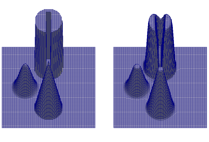
3.2 Advection of a discontinous function with curvature

In this test case, the transport equations are solved in the unit square $\Omega=(0,1)^{2}$ with velocity field $\boldsymbol{u}=(1,0)$, i.e. steady translation in the $x$-direction (which is the direction of discontinuity in the finite element space). The initial condition is

$$\theta=\left\{\begin{array}[]{cc}4y(1-y)+1&\mbox{ if }0.2<x<0.4,\\ 4y(1-y)&\mbox{ otherwise. }\end{array}\right.$$ (31)

This test case is challenging because the height of the ``plateau'' next to the continuity varies as a function of $y$ (i.e., in the direction tangential to the discontinuity); this means that the behaviour of the limiter is more sensitive to the process of obtaining local bounds.

The equations are integrated until $t=0.4$ in a $100\times 100$ square grid and Courant number 0.3. The results are showing in Figure Embedded discontinuous Galerkin transport schemes with localised limiters. One can see qualitatively that the degradation in the solution due to the limiter and numerical errors is not too great.

;
Figure 4: Results from the test case in Section 3.2. Left: The initial condition. Right: The solution at time $t=0.4$.
; where $\boldsymbol{x}=(x,y)$; at fixed timestep $\Delta t=0.000856898$; $C_{0}$)
Abstract

Motivated by finite element spaces used for representation of temperature in the compatible finite element approach for numerical weather prediction, we introduce locally bounded transport schemes for (partially-)continuous finite element spaces. The underlying high-order transport scheme is constructed by injecting the partially-continuous field into an embedding discontinuous finite element space, applying a stable upwind discontinuous Galerkin (DG) scheme, and projecting back into the partially-continuous space; we call this an embedded DG transport scheme. We prove that this scheme is stable in $L^{2}$ provided that the underlying upwind DG scheme is. We then provide a framework for applying limiters for embedded DG transport schemes. Standard DG limiters are applied during the underlying DG scheme. We introduce a new localised form of element-based flux-correction which we apply to limiting the projection back into the partially-continuous space, so that the whole transport scheme is bounded. We provide details in the specific case of tensor-product finite element spaces on wedge elements that are discontinuous P1/Q1 in the horizontal and continuous in the . The framework is illustrated with numerical tests.

keywords:
Discontinuous Galerkin , slope limiters , flux corrected transport , convection-dominated transport , numerical weather prediction
journal: Journal of Computational Physics

1 Introduction

, this is being driven by the need to move away from the latitude-longitude grids which are currently used in NWP models, since they prohibit parallel scalability . methods rely on choosing compatible finite element spaces for the various prognostic fields (velocity, density, temperature, etc.), in order to avoid spurious numerical wave propagation that pollutes the numerical solution on long time scales. In particular, in three dimensional models, this calls for the velocity space to be a div-conforming space such as Raviart-Thomas, and the density space is the corresponding discontinuous space. Many current operational forecasting models, such as the Met Office Unified Model (Davies et al., 2005), use a Charney-Philips grid staggering in the vertical, to avoid a spurious mode in the vertical. When translated into the framework of compatible finite element spaces, this requires the temperature space to be a tensor product of discontinuous functions in the horizontal and continuous functions in the vertical (more details are given below). Physics/dynamics coupling then requires that other tracers (moisture, chemical species etc.) also use the same finite element space as temperature.

A critical requirement for numerical weather prediction models is that the transport schemes for advected tracers do not lead to the creation of new local maxima and minima, since their coupling back into the dynamics is very sensitive. In the compatible finite element framework, this calls for the development of limiters for partially-continuous finite element spaces. Since there is a well-developed framework for limiters for discontinuous Galerkin methods , in this paper we pursue the three stage approach of (i) injecting the solution into an embedding discontinuous finite element space at the beginning of the timestep, then (ii) applying a standard discontinuous Galerkin timestepping scheme, before finally (iii) projecting the solution back into the partially continuous space. If the discontinuous Galerkin scheme is combined with a slope limiter, the only step where overshoots and undershoots can occur is in the final projection. In this paper we describe a localised limiter for the projection stage, which is a modification of element-based limiters (Löhner et al., 1987; Kuzmin and Turek, 2002) previously applied to remapping in Löhner (2008); Kuzmin et al. (2010). This leads to a locally bounded advection scheme when combined with the other steps.

The rest of the paper is structured as follows. The problem is formulated in Section 2. In particular, more detail on the finite element spaces is provided in Section 2.1. The embedded discontinuous Galerkin schemes are introduced in Section 2.2; it is also shown that these schemes are stable if the underlying discontinuous Galerkin scheme is stable. The limiters are described in Section 2.3. In Section 3 we provide some numerical examples. Finally, in Section 4 we provide a summary and outlook.

2 Formulation

2.1 Finite element spaces

We begin by defining the partially continuous finite element spaces under consideration. In three dimensions, the element domain is constructed as the tensor product of a two-dimensional horizontal element domain (a triangle or a quadrilateral) and a one-dimensional vertical element domain (i.e., an interval); we obtain triangular prism or hexahedral element domains aligned with the vertical direction. For a vertical slice geometry in two dimensions (frequently used in testcases during model development), the horizontal domain is also an interval, and we obtain quadrilateral elements aligned with the vertical direction.

To motivate the problem of transport schemes for a partially continuous finite element space, we first consider a compatible finite element scheme that uses a discontinuous finite element space for density. This is typically formed as the tensor product of the $DG_{k}$ space in the horizontal (degree $k$ polynomials on triangles or bi-$k$ polynomials on quadrilaterals, allowing discontinuities between elements) and the $DG_{l}$ space in the vertical. We consider the case where the same degree is chosen in horizontal and vertical, i.e. $k=l$, although there are no restrictions in the framework. We will denote this space as $DG_{k}\times DG_{k}$.

In the compatible finite element framework, the vertical velocity space is staggered in the vertical from the pressure space; the staggering is selected by requiring that the divergence (i.e., the vertical derivative of the vertical velocity) maps from the vertical velocity space to the pressure space. This means that vertical velocity is stored as a field in $DG_{k}\times CG_{k+1}$ (where $CG_{k+1}$ denotes degree $k+1$ polynomials in each interval element, with $C^{0}$ continuity between elements). To avoid spurious hydrostatic pressure modes, one may then choose to store (potential) temperature in the same space as vertical velocity (this is the finite element version of the Charney-Phillips staggering). Details of how to automate the construction of these finite element spaces within a code generation framework are provided in McRae et al. (2015).

[Uncaptioned image]

Monotonic transport schemes for temperature are often required, particularly in challenging testcases such as baroclinic front generation. Further, dynamics-physics coupling requires that other tracers such as moisture must be stored at the same points as temperature; many of these tracers are involved in parameterisation calculations that involve switches and monotonic advection is required to avoid spurious formation of rain patterns at the gridscale, for example. Hence, we must address the challenge of monotonic advection in the partially continuous $DG_{k}\times CG_{k+1}$ space.

In this paper, we shall concentrate on the case of $DG_{1}\times CG_{2}$. This is motivated by the fact that we wish to use standard DG upwind schemes where the advected tracer is simply evaluated on the upwind side; the lowest order space $DG_{0}\times CG_{1}$ leads to a first order scheme in this case. We may return to higher order spaces in future work.

2.2 Embedded Discontinuous Galerkin schemes

[Uncaptioned image]

2.3 Bounded transport

Next we wish to add limiters to the scheme. This is done in two stages. To control these unwanted oscillations, we apply a (conservative) flux correction to the projection, referred to as flux corrected remapping (Kuzmin et al., 2010)

2.3.1 Slope limiter

In this paper we used the vertex-based slope limiter of Kuzmin (2010). This limiter is both very easy to implement, and supports a treatment of the quadratic structure in the vertical. The basic idea for is to write

$$\theta=\bar{\theta}+\Delta\theta,$$ (8)

where $\bar{\theta}$ is the projection of $\theta$ into $DG_{0}$, i.e. in each element $\bar{\theta}$ is the element-averaged value of $\theta$. Then, for each vertex $i$ in the mesh, we compute maximum and minimum bounds $\theta_{\max,i}$ and $\theta_{\min,i}$ by computing the maximum and minimum values of $\bar{\theta}$ over all the elements that contain that vertex, respectively. In each element $e$ we then compute a constant $0\leq\alpha_{e}\leq 1$ such that the value of

$$\theta_{\min,i}\leq\theta_{e}(\boldsymbol{x}_{i})=\bar{\theta}_{e}+\alpha_{e}(\Delta\theta)_{e}(\boldsymbol{x}_{i})\leq\theta_{\max,i},$$ (9)

at each vertex $i$ contained by element $e$. The optimal value of the correction factor $\alpha_{e}$ can be determined using the formula of Barth and Jespersen (1989)

$$\alpha_{e}=\min\limits_{i\in{\cal N}_{e}}\left\{\begin{array}[]{ll}\min\left\{1,\frac{\theta_{\max,i}-\bar{\theta}_{e}}{\theta_{e,i}-\bar{\theta}_{e}}\right\}&\mbox{if}\quad\theta_{e,i}-\bar{\theta}_{e}>0,\\[2.84544pt] 1&\mbox{if}\quad\theta_{e,i}-\bar{\theta}_{e}=0,\\[0.0pt] \min\left\{1,\frac{\theta_{\min,i}-\bar{\theta}_{e}}{\theta_{e,i}-\bar{\theta}_{e}}\right\}&\mbox{if}\quad\theta_{e,i}-\bar{\theta}_{e}<0,\end{array}\right.$$ (10)

where ${\cal N}_{e}$ is the set of vertices of element $e$ and $\theta_{e,i}=\bar{\theta}_{e}+(\Delta\theta)_{e}(\boldsymbol{x}_{i})$ is the unconstrained value of the $DG_{1}$ shape function at the $i$-th vertex.

$$\theta={\bar{\theta}}+(\theta_{1}-\bar{\theta})+(\theta-\theta_{1}),$$ (11)

Then, $\frac{\partial\theta}{\partial z}\in DG_{1}\times DG_{1}$ whilst $\frac{\partial\theta_{1}}{\partial z}\in DG_{1}\times DG_{0}$.

First, we limit the quadratic component in the vertical (the third term in Equation (11)), performing the following steps.

  1. 1.

    In each element, compute $\frac{\partial\theta_{1}}{\partial z}$, and If the quadratic component $\theta-\theta_{1}$ is limited to zero then $\frac{\partial\theta_{1}}{\partial z}$ will become equal to $\overline{\frac{\partial\theta_{1}}{\partial z}}$.

  2. 2.

    In each column, at each vertex $i$, compute bounds $\frac{\partial\theta}{\partial z}|_{\min,i}$ and $\frac{\partial\theta}{\partial z}|_{\max,i}$ by taking the maximum value of $\overline{\frac{\partial\theta_{1}}{\partial z}}$ at that vertex in the elements in the column.

  3. 3.

    In each element, compute element correction factors $\alpha_{1,e}$ according to

    $$\alpha_{1,e}=\min\limits_{i\in{\cal N}_{e}}\left\{\begin{array}[]{ll}\min\left\{1,\frac{\frac{\partial\theta}{\partial z}|_{\max,i}-\overline{\frac{\partial\theta}{\partial z}}|_{e,i}}{\frac{\partial\theta}{\partial z}_{e,i}-\overline{\frac{\partial\theta}{\partial z}}|_{e,i}}\right\}&\mbox{if}\quad\frac{\partial\theta}{\partial z}|_{e,i}-\overline{\frac{\partial\theta}{\partial z}}|_{e,i}>0,\\[2.84544pt] 1&\mbox{if}\quad-\overline{\frac{\partial\theta}{\partial z}}|_{e,i}=0,\\[0.0pt] \min\left\{1,\frac{\frac{\partial\theta}{\partial z}|_{\min,i}-\overline{\frac{\partial\theta}{\partial z}}|_{e,i}}{\frac{\partial\theta}{\partial z}|_{e,i}-\overline{\frac{\partial\theta}{\partial z}}|_{e,i}}\right\}&\mbox{if}\quad\frac{\partial\theta}{\partial z}|_{e,i}-\overline{\frac{\partial\theta}{\partial z}}|_{e}<0.\end{array}\right.$$ (12)

This approach can also be extended to meshes in spherical geometry for which all side walls are parallel to the radial direction111Such meshes arise when terrain following grids are used in spherical geometry., having replaced $\frac{\partial}{\partial z}$ by the radial derivative.

Second, we apply the vertex-based limiter to the $DG_{1}\times DG_{1}$ component $\theta_{1}$, obtaining limiting constants $\alpha_{0}$. We then finally evaluate

$$\theta\mapsto\theta=\bar{\theta}+\alpha_{0}(\theta_{1}-\bar{\theta})+\alpha_{1}(\theta-\theta_{1}).$$ (13)

To reduce diffusion of smooth extrema, it was recommended in Kuzmin (2010) to recompute the $\alpha_{0}$ coefficients according to

$$\alpha_{0,e}\mapsto\max(\alpha_{0,e},\alpha_{1,e}).$$ (14)

However, this does not work in the case of $DG_{1}\times DG_{2}$ since there is no quadratic component in the horizontal direction, and hence nonsmooth extrema in the horizontal direction will not be detected. A possible remedy is to use $\alpha_{0,e}$ for the horizontal gradient and $\max(\alpha_{0,e},\alpha_{1,e})$ for the vertical gradient or to limit the directional derivatives separately using an anisotropic version of the vertex-based slope limiter (Kuzmin et al. (2015)).

2.3.2 Flux corrected remapping

(15)

where the lumped mass $M$ is defined by

$$M_{i}=\int_{\Omega}\phi_{i}\operatorname{d}x,$$ (16)

the projection matrix $Q$ is defined by $\{\psi_{i}\}_{i=1}$ is a basis for $DG_{1}\times DG_{1}$

The lumped mass $M$ and projection matrix $Q$ both have strictly positive entries. This means that for each $1\leq i\leq n$, the basis coefficient $\theta^{L}_{i}$ is a weighted average of values of coming from elements that lie in $S(i)$, the support of $\phi_{i}$. The weights are all positive, and hence the value of $\theta^{L}_{i}$ is bounded by the maximum and minimum values of in $S(i)$. Hence, no new maxima or minima appear in the low order solution.

consistent mass counterpart of (15) is given by

$$\sum_{j=1}^{n}M_{ij}\theta_{j}^{H}=\int_{\Omega}\phi_{i}\hat{\theta}\operatorname{d}x,\quad i=1,\ldots,n,$$ (18)

where

$$M_{ij}=\int_{\Omega}\phi_{i}\phi_{j}\operatorname{d}x.$$ (19)

First, by repeated addition and subtraction of terms, we write (with no implied sum over the index $i$) This can be decomposed into elements to obtain

We can then choose element limiting constants $\alpha^{e}$ to get

$$M_{i}\theta^{H}_{i}=\sum_{e}\left(M_{i}^{e}\theta^{L}_{i}+\alpha_{e}f_{i}^{e}\right),$$ (26)

where $0\leq\alpha_{e}\leq 1$ is a limiting constant for each element which is chosen to satisfy vertex bounds obtained from the nodal values of $\hat{\theta}$.

The bounds in each vertex are obtained as follows. First element bounds $\theta_{\max}^{e}$ and $\theta_{\min}^{e}$ are obtained from $\hat{\theta}$ by maximising/minimising over the vertices of element $e$. Then for each vertex $i$, maxima/minima are obtained by maximising/minimising over the elements containing the vertex:

$$\theta_{\max,i}=\max_{e}\theta_{\max}^{e},\quad\theta_{\min,i}=\min_{e}\theta_{\min}^{e}.$$ (27)

The correction factor $\alpha_{e}$ is chosen so as to enforce the local inequality constraints

$$M_{i}^{e}\theta_{\min,i}\leq M_{i}^{e}\theta_{i}^{L}+\alpha_{e}f_{i}^{e}\leq M_{i}^{e}\theta_{\max,i}$$ (28)

Summing over all elements, one obtains the corresponding global estimate

$$M_{i}\theta_{\min,i}\leq M_{i}\theta_{i}^{L}+\sum_{e}\alpha_{e}f_{i}^{e}\leq M_{i}\theta_{\max,i},$$ (29)

which proves that the corrected value $\theta_{i}^{C}:=\theta_{i}^{L}+\frac{1}{M_{i}}\sum_{e}\alpha_{e}f_{i}^{e}$ is bounded by $\theta_{\max,i}$ and $\theta_{\min,i}$.

To enforce the above maximum principles, we limit the element contributions $f_{i}^{e}$ using

$$\alpha_{e}=\min\limits_{i\in{\cal N}_{e}}\left\{\begin{array}[]{ll}\min\left\{1,\frac{M_{i}^{e}(\theta_{\max,i}-\theta^{L}_{i})}{f_{i}^{e}}\right\}&\mbox{if}\quad f_{i}^{e}>0,\\[2.84544pt] 1&\mbox{if}\quad f_{i}^{e}=0,\\[0.0pt] \min\left\{1,\frac{M_{i}^{e}(\theta_{\min,i}-\theta^{L}_{i})}{f_{i}^{e}}\right\}&\mbox{if}\quad f_{i}^{e}<0.\end{array}\right.$$ (30)

This definition of $\alpha_{e}$ corresponds to a localised version of the element-based multidimensional FCT limiter ((Löhner et al., 1987; Kuzmin and Turek, 2002)) and has the same structure as formula (10) for the correction factors that we used to constrain the $DG_{1}$ approximation.

3 Numerical Experiments

Refer to caption

Figure 3: Solid body rotation test (Section 3.1) on a 100$\times$100 grid. Solution is interpolated to a $DG_{1}$ discontinuous field before plotting. Left: initial condition. Right: Solution after one rotation. The solution is free from over- and undershoots and exhibits comparable numerical dissipation to discontinuous Galerkin methods combined with limiters.

In this section, we provide some numerical experiments demonstrating the localised limiter for embedded Discontinuous Galerkin schemes.

3.1 Solid body rotation

In this standard test case, the transport equations are solved in the unit square $\Omega=(0,1)^{2}$ with velocity field $\boldsymbol{u}(x,y)=(0.5-y,x-0.5)$, i.e. a solid body rotation in anticlockwise direction about the centre of the domain, so that the exact solution at time $t=2\pi$ is equal to the initial condition. The initial condition is chosen to be the standard hump-cone-slotted cylinder configuration defined in LeVeque (1996), and solved on a regular mesh with element width $h=1/100$ . The result, shown in Figure 3, is comparable with the result for the discontinuous Galerkin vertex-based limiter shown in Figure 2 of Kuzmin (2010); it is free from over- and undershoots and exhibits a similar amount of numerical diffusion.

[Uncaptioned image] [Uncaptioned image]

3.3 Convergence test: deformational flow

In this test, we consider the advection of a smooth function by a deformational flow field that is reversed so that the function at time $t=1$ is equal to the initial condition. As is standard for this type of test, we add a translational component to the flow and solve the problem with periodic boundary conditions to eliminate the possibility of fortuitous error cancellation due to the time reversal.

The transport equations are solved in a unit square, with periodic boundary conditions in the $x$-direction. The initial condition is

$$\theta(\boldsymbol{x},0)=0.25(1+\cos(r)),\quad r=\min\left(0.2,\sqrt{(x-0.3)^{2}+(y-0.5)^{2}}/0.2\right),$$

and the velocity field is

$$\boldsymbol{u}(\boldsymbol{x},t)=\left(1-5(0.5-t)\sin(2\pi(x-t))\cos(\pi y),5(0.5-t)\cos(2\pi(x-t))\sin(\pi y)\right),$$

. The problem was solved on a sequence of regular meshes with square elements , and the $L^{2}$ error was computed. A plot of the errors is provided in Figure 5. As expected, we obtain second-order convergence (the quadratic space in the vertical does not enhance convergence rate because the full two-dimensional quadratic space is not spanned).

Refer to caption

ΔxΔ𝑥\Delta x L2superscript𝐿2L^{2} 
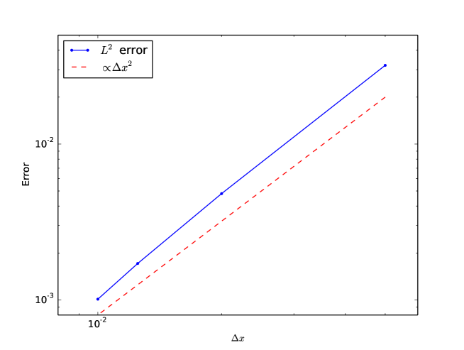
error 0.05 0.0319911 0.02 0.0048104 0.0125 0.0017125 0.01 0.0010108

Figure 5: Convergence plot for deformational flow experiment (Section 3.3) showing second order convergence, and a table of error values.

4 Summary and Outlook

In this paper we described a limited transport scheme for partially-continuous finite element spaces. Motivated by numerical weather prediction applications, where the finite element space for temperature and other tracers is imposed by hydrostatic balance and wave propagation properties, we focussed particularly on the case of tensor-product elements that are continuous in the vertical direction but discontinuous in the horizontal. However, the entire methodology applies to standard finite element spaces. The transport scheme was demonstrated in terms of convergence rate on smooth solutions and dissipative behaviour for non-smooth solutions in some standard testcases.

Having a bounded transport scheme for tracers is a strong requirement for numerical weather prediction algorithms; the development of our scheme advances the practical usage of the compatible finite element methods described in the introduction. The performance of this transport scheme applied to temperature in a fully coupled atmosphere model will be evaluated in 2D and 3D testcases as part of the ``Gung Ho'' UK Dynamical Core project in collaboration with the Met Office. In the case of triangular prism elements we anticipate that it may be necessary to modify the algorithm above to limit the time derivatives as described in Kuzmin (2013).

A key novel aspect of our transport scheme is the localised element-based FCT limiter. This limiter has much broader potential for use in FCT schemes for continuous finite element spaces, which will be explored and developed in future work.

5 Acknowledgements

Colin Cotter acknowledges funding from NERC grant NE/K006789/1. Dmitri Kuzmin acknowledges funding from DFG grant KU 1530/12-1.

References

  • Bao et al. (2015) Bao, L., Klöfkorn, R., Nair, R. D., 2015. Horizontally explicit and vertically implicit (HEVI) time discretization scheme for a discontinuous Galerkin nonhydrostatic model. Monthly Weather Review 143 (3), 972–990.
  • Barth and Jespersen (1989) Barth, T., Jespersen, D., 1989. The design and application of upwind schemes on unstructured meshes. AIAA Paper 89-0366.
  • Biswas et al. (1994) Biswas, R., Devine, K., Flaherty, J. E., 1994. Parallel adaptive finite element methods for conservation laws. Appl. Numer. Math. 14, 255–285.
  • Brdar et al. (2013) Brdar, S., Baldauf, M., Dedner, A., Klöfkorn, R., 2013. Comparison of dynamical cores for NWP models: comparison of COSMO and Dune. Theoretical and Computational Fluid Dynamics 27 (3-4), 453–472.
  • Burbeau et al. (2001) Burbeau, A., Sagaut, P., Bruneau, C.-H., 2001. A problem-independent limiter for high-order Runge-Kutta discontinuous Galerkin methods. J. Comput. Phys. 169, 111–150.
  • Cockburn and Shu (2001) Cockburn, B., Shu, C.-W., 2001. Runge–Kutta discontinuous Galerkin methods for convection-dominated problems. Journal of Scientific Computing 16 (3), 173–261.
  • Cotter and Shipton (2012) Cotter, C., Shipton, J., 2012. Mixed finite elements for numerical weather prediction. Journal of Computational Physics 231 (21), 7076–7091.
  • Cotter and Thuburn (2014) Cotter, C. J., Thuburn, J., 2014. A finite element exterior calculus framework for the rotating shallow-water equations. Journal of Computational Physics 257, 1506–1526.
  • Davies et al. (2005) Davies, T., Cullen, M., Malcolm, A., Mawson, M., Staniforth, A., White, A., Wood, N., 2005. A new dynamical core for the Met Office's global and regional modelling of the atmosphere. Quarterly Journal of the Royal Meteorological Society 131 (608), 1759–1782.
  • Dennis et al. (2011) Dennis, J., Edwards, J., Evans, K. J., Guba, O., Lauritzen, P. H., Mirin, A. A., St-Cyr, A., Taylor, M. A., Worley, P. H., 2011. CAM-SE: A scalable spectral element dynamical core for the Community Atmosphere Model. International Journal of High Performance Computing Applications, 1094342011428142.
  • Fournier et al. (2004) Fournier, A., Taylor, M. A., Tribbia, J. J., 2004. The spectral element atmosphere model (SEAM): High-resolution parallel computation and localized resolution of regional dynamics. Monthly Weather Review 132 (3), 726–748.
  • Giraldo et al. (2013) Giraldo, F. X., Kelly, J. F., Constantinescu, E., 2013. Implicit-explicit formulations of a three-dimensional nonhydrostatic unified model of the atmosphere (NUMA). SIAM Journal on Scientific Computing 35 (5), B1162–B1194.
  • Guba et al. (2014) Guba, O., Taylor, M., St-Cyr, A., 2014. Optimization-based limiters for the spectral element method. Journal of Computational Physics 267, 176–195.
  • Hoteit et al. (2004) Hoteit, H., Ackerer, P., Mosé, R., Erhel, J., Philippe, B., 2004. New two-dimensional slope limiters for discontinuous Galerkin methods on arbitrary meshes. Int. J. Numer. Meth. Engrg. 61, 2566–2593.
  • Kelly and Giraldo (2012) Kelly, J. F., Giraldo, F. X., 2012. Continuous and discontinuous Galerkin methods for a scalable three-dimensional nonhydrostatic atmospheric model: Limited-area mode. Journal of Computational Physics 231 (24), 7988–8008.
  • Krivodonova et al. (2004) Krivodonova, L., Xin, J., Remacle, J.-F., Chevaugeon, N., Flaherty, J., 2004. Shock detection and limiting with discontinuous Galerkin methods for hyperbolic conservation laws. Appl. Numer. Math. 48, 323–338.
  • Kuzmin (2010) Kuzmin, D., 2010. A vertex-based hierarchical slope limiter for p-adaptive discontinuous Galerkin methods. Journal of Computational and Applied Mathematics 233 (12), 3077–3085.
  • Kuzmin (2013) Kuzmin, D., 2013. Slope limiting for discontinuous Galerkin approximations with a possibly non-orthogonal Taylor basis. International Journal for Numerical Methods in Fluids 71 (9), 1178–1190.
  • Kuzmin et al. (2015) Kuzmin, D., Kosík, A., Aizinger, V., 2015. Anisotropic slope limiting in discontinuous Galerkin methods for transport equations, paper in preparation.
  • Kuzmin et al. (2010) Kuzmin, D., Möller, M., Shadid, J. N., Shashkov, M., 2010. Failsafe flux limiting and constrained data projections for equations of gas dynamics. Journal of Computational Physics 229 (23), 8766–8779.
  • Kuzmin and Turek (2002) Kuzmin, D., Turek, S., 2002. Flux correction tools for finite elements. Journal of Computational Physics 175, 525–558.
  • LeVeque (1996) LeVeque, R., 1996. High-resolution conservative algorithms for advection in incompressible flow. SIAM J. Numer. Anal. 33, 627–665.
  • Löhner (2008) Löhner, R., 2008. Applied CFD Techniques: An Introduction Based on Finite Element Methods. John Wiley & Sons.
  • Löhner et al. (1987) Löhner, R., Morgan, K., Peraire, J., Vahdati, M., 1987. Finite element flux-corrected transport (FEM–FCT) for the Euler and Navier–Stokes equations. International Journal for Numerical Methods in Fluids 7 (10), 1093–1109.
  • Marras et al. (2012) Marras, S., Kelly, J. F., Giraldo, F. X., Vázquez, M., 2012. Variational multiscale stabilization of high-order spectral elements for the advection–diffusion equation. Journal of Computational Physics 231 (21), 7187–7213.
  • Marras et al. (2015) Marras, S., Kelly, J. F., Moragues, M., Müller, A., Kopera, M. A., Vázquez, M., Giraldo, F. X., Houzeaux, G., Jorba, O., 2015. A review of element-based Galerkin methods for numerical weather prediction: Finite elements, spectral elements, and discontinuous Galerkin. Archives of Computational Methods in Engineering, 1–50.
  • Marras et al. (2013) Marras, S., Moragues, M., Vázquez, M., Jorba, O., Houzeaux, G., 2013. Simulations of moist convection by a variational multiscale stabilized finite element method. Journal of Computational Physics 252, 195–218.
  • McRae et al. (2015) McRae, A. T., Bercea, G.-T., Mitchell, L., Ham, D. A., Cotter, C. J., 2015. Automated generation and symbolic manipulation of tensor product finite elements. Submitted, arXiv preprint arXiv:1411.2940.
  • McRae and Cotter (2014) McRae, A. T., Cotter, C. J., 2014. Energy-and enstrophy-conserving schemes for the shallow-water equations, based on mimetic finite elements. Quarterly Journal of the Royal Meteorological Society 140 (684), 2223–2234.
  • Shu and Osher (1988) Shu, C.-W., Osher, S., 1988. Efficient implementation of essentially non-oscillatory shock-capturing schemes. Journal of Computational Physics 77 (2), 439–471.
  • Staniforth et al. (2013) Staniforth, A., Melvin, T., Cotter, C. J., 2013. Analysis of a mixed finite-element pair proposed for an atmospheric dynamical core. Quarterly Journal of the Royal Meteorological Society 139 (674), 1239–1254.
  • Staniforth and Thuburn (2012) Staniforth, A., Thuburn, J., 2012. Horizontal grids for global weather and climate prediction models: a review. Quarterly Journal of the Royal Meteorological Society 138 (662), 1–26.
  • Thomas and Loft (2005) Thomas, S. J., Loft, R. D., 2005. The NCAR spectral element climate dynamical core: Semi-implicit Eulerian formulation. Journal of Scientific Computing 25 (1), 307–322.
  • Tu and Aliabadi (2005) Tu, S., Aliabadi, S., 2005. A slope limiting procedure in discontinuous Galerkin finite element method for gasdynamics applications. Int. J. Numer. Anal. Model. 2, 163–178.
  • Zhang and Shu (2011) Zhang, X., Shu, C.-W., 2011. Maximum-principle-satisfying and positivity-preserving high-order schemes for conservation laws: survey and new developments. In: Proceedings of the Royal Society of London A: Mathematical, Physical and Engineering Sciences. The Royal Society, p. rspa20110153.