Qualitative and Quantitative Stability Analysis of Penta-rhythmic Circuits

Abstract

Inhibitory circuits of relaxation oscillators are often-used models for the dynamics of biological networks. We present a qualitative and quantitative stability analysis of such a circuit constituted by three reciprocally coupled oscillators of a Fitzhugh-Nagumo type as nodes. Depending on inhibitory strengths, and parameters of individual oscillators, the circuit exhibits polyrhythmicity of up to five simultaneously stable rhythms. With methods of bifurcation analysis and phase reduction, we investigate qualitative changes in stability of these circuit rhythms for a wide range of parameters. Furthermore, we quantify how robustly rhythms are maintained under random perturbations by monitoring phase diffusion in the circuit. Our findings allow us to describe how circuit dynamics relate to dynamics of individual nodes. We also find that quantitative and qualitative stability of polyrhythmicity do not always align.

I Introduction

Relaxation oscillators have become a base for constituting coupled systems that generate a variety of self-sustained rhythms. These types of oscillators are used to model heart beats [1], cellular membrane dynamics [2], electrical and mechanical systems [3, 4], harmful algae bloom [5], regulatory genetic networks [6, 7], and the population dynamics of pest cycles of forests [8].

Simple relaxation oscillations are formed by two essential variables: one activity variable assumes active and inactive states, and one recovery variable regulates and completes the activity cycle by destabilizing the activity states, and thus leading to recurrent switching. The activity variable exhibits dynamic hysteresis in which the state of activity is bi-stable if the recovery variable is held constant. For example in neuronal dynamics, the cell membrane voltage determines the state of neuronal activity. The state becomes active as the voltage depolarizes. This depolarization occurs when the potassium-ion conductance, i.e. the recovery variable, falls below a threshold. In return, the depolarized, active membrane voltage opens voltage-dependent K⁺-gates causing the K⁺-conductance to increase. Such increases beyond another threshold cause the active state of the membrane voltage to destabilize, and thereby to complete the cycle. While more detailed models can exhibit other complex types of neuronal activity, such as sub-threshold oscillations and bursting [9, 10, 11, 12, 13], this mechanism of hysteresis, which guides the relaxation oscillations, is retained.

Coupling among relaxation oscillators is introduced through interactions of their activity variables. Prominent biological examples of coupled systems include neuronal populations connected by chemical synapses and gap junctions [14, 15, 16], as well as single-cell organisms communicating via signaling molecules [17]. We distinguish two types of connections: excitatory connections promote and support the active state, and inhibitory connections repress the active state and hold the inactive state of the oscillator. Note that neuronal gap junctions and other types of diffusive coupling do not fall into either of these categories.

Networked oscillators typically show a degree of coordination among their individual cycles. Reciprocal excitation between two oscillators leads to their synchrony, whereas inhibition forces them to oscillate in anti-phase [18]. Moreover, slow inhibition can promote synchrony in two coupled oscillatory neurons [18, 15, 19, 20], while fast, non-delayed inhibition allows for synchronous bursting dynamics due to spike interactions [21, 22]. Generation of robust network rhythms is of particular relevance for neural ensembles that control the dynamics of motor patterns. These central pattern generators (CPGs), described in the next section, largely inspire the research presented in this work.

I.1 Dynamics of Central Pattern Generators

Small neuronal networks of interconnected relaxation oscillators have been identified in a number of invertebrate CPGs [23, 24, 25]. These networks are structurally equal in individuals of the same species, and show characteristic differences across related species [25]. A function of the network connectivity is to maintain a single rhythmic activity pattern of the oscillators, and to ensure resilience of the pattern against disturbances. Indeed, computationally extensive modelling studies of a three-node CPG that controls rhythmic motion in the stomach of lobsters revealed that a wide range of circuit parameters could produce the same rhythmic output [26, 27, 28]. This invariance of pattern generation with respect to parameter changes highlights the robustness of the network structure to stably produce certain rhythms.

More complex CPGs support multiple rhythms to efficiently perform multiple functions [29] (see Ref. [30] for a review on multistability). To study the dynamics of these CPGs, the state space of each circuit configuration needs to be analyzed for multistability and polyrhythmicity. Arguably, the brute-force methods used in aforementioned lobster studies are numerically impractical in this case, and other methods are therefore needed. One potentially viable approach relies on techniques of qualitative theory to mechanistically understand and categorize the relation between circuitry and rhythmogenesis [31, 32, 33, 34, 35].

In our recent qualitative studies on circuits consisting of several endogenous bursters, we have learned that (1) the duty cycle of individual neurons strongly affects circuit rhythmicity [12]; (2) variations in coupling strength among the bursters lead to predictable bifurcations of rhythms [35]; (3) strong reciprocal inhibition can make network rhythms vulnerable to perturbations such as noise [37]. Based on these results, we have been able to better understand the swim CPG of a sea slug, Melibe leonina [34, 38]. Our continuing goal is to develop the theory of rhythmogenesis to predict changes in rhythm stability, and to determine the robustness of rhythms in an oscillatory network given its circuitry.

In this paper, we generalize previous results to three-node circuits constituted of generic relaxation oscillators with relevance outside of computational neuroscience. We adopt and counterpose a variety analysis techniques for polyrythmic circuits and highlight their individual strengths. Our complimentary techniques of phase reduction, bifurcation theory, perturbation theory, and stochastic dynamics lets us describe a near-maximal range of dynamical regimes including different separations of time scale between activity and recovery variables, bifurcations in individual nodes, and a range of coupling strengths from weak to strong. We find that stability and robustness of circuit rhythms strongly depend on the parameters of oscillators in the circuit. In the vicinity of their individual bifurcations, abrupt changes in the circuit dynamics are observed. Furthermore, we demonstrate that qualitative and quantitative stability of polyrhythms do not align completely, thereby leading us to new hypotheses concerning polyrhythmic circuits. Our results strengthen and generalize previous findings obtained with Hodgkin-Huxley-type neuronal circuits. Moreover, synthesizing the outcome of various analysis techniques allows us to specify conditions under which an individual technique may efficiently extract particular dynamical features of stability for a given polyrhythmic circuit.

Note that resilience of the circuit to retain a rhythm under external disturbances is analyzed in two ways, in this article, using the terms stability and robustness. Stability describes the response of the circuit dynamics to infinitesimal perturbations. Robustness describes this response to finite, stochastic perturbations.

II Methods

II.1 Circuit Dynamics

We consider a circuit of three Fitzhugh-Nagumo like relaxation oscillators that are identical and coupled all-to-all. The circuit dynamics are governed by the following equations:

$$\begin{aligned} \dot{V}_{i}&=V_{i}-V_{i}^{3}+I-x_{i}-g\sum_{i\neq j}G(V_{i},V_{j})\leavevmode\nobreak\ ,\\ \dot{x}_{i}&=\varepsilon\left[x_{\infty}(V_{i})-x_{i}\right]\leavevmode\nobreak\ ,\qquad i,j=1,\,2,\,3\leavevmode\nobreak\ .\end{aligned}$$ (1)

The state of each individual node is described by the activity variable $V_{i}$ and recovery variable $x_{i}$. Node $j$ is called active if $V_{j}$ exceeds the activation threshold at $V_{j}=0$. Active oscillators repress their coupling partners towards the inactive state ($V_{i}<0$). This interaction stabilizes certain activity patterns in the circuit dynamics as demonstrated with two sample trajectories in Fig. 1. Starting from arbitrary initial conditions, the phases of activity in each oscillator realign and converge to a stable circuit rhythm.

The family of circuits is altered by the parameters, nullcline shift $I$ and inhibitory strength $g$ discussed in Sec. II.2, as well as time-scale parameter $\varepsilon$. Small values of $\varepsilon$, e.g. $\varepsilon=0.1$, indicate well-separate time scales between the dynamics of $V$ and $x$.

Nodes are coupled via a sigmoidal coupling function

$$G(V_{i},V_{j})=\frac{V_{i}-E}{1+e^{-100\,V_{j}}}\leavevmode\nobreak\ ,$$

with $E=-1.5$. This choice of $E$ makes coupling inhibitory. The equilibrium state of the recovery variable is also represented by the sigmoidal function:

$$x_{\infty}(V)=\frac{1}{1+e^{-10\,V}}\leavevmode\nobreak\ .$$

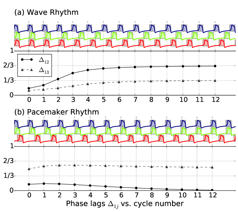
Figure 1: (Color online) Rhythms in the three-node circuit. Oscillations of $V$-variables (top traces) converge to one of the wave rhythms (a), and pacemaker rhythms (b), both simultaneously stable. The convergence is visible in the dynamics of phase lags, $\Delta=(\Delta_{12},\Delta_{13})$, that approach the characteristic fixed points $\Delta=(2/3,1/3)$, and $(0,1/2)$ in panel (a) and (b), respectively. Boxes denote active states. Parameters: $g=0.005$, $I=0.4$, $\varepsilon=0.17$.

In a neuroscience context, Eq. (1) represents a phenomenological model of neuronal dynamics [2, 39]. Variables $V_{i}$ and $x_{i}$ describe the membrane voltage and a voltage-dependent K⁺-conductance, while the coupling function models fast inhibitory ($V_{j}>E$) synapses [14].

II.2 Release, Escape, and Coupling

We investigate the circuit dynamics with individual node dynamics set at a range of parameters in between two bifurcations controlled by $I$. Let us describe individual dynamics at these bifurcations in the $(V,x)$-plane with a special emphasis placed on the two nullclines : the $V$-nullcline is the cubic parabola on which $\dot{V}=0$, and the $x$-nullcline is a sigmoidal graph on which $\dot{x}=0$; both nullclines are shown in Fig. 2. Nullclines coordinate the dynamics; whenever the state is above the $x$-nullcline, $x(t)$ increases and whenever the state lies to the right of the $V$-nullcline, $V(t)$ decreases, and vice versa. As shown in the figure, this leads to self-sustained relaxation oscillations in which the trajectory periodically bypasses the lower and upper fold or knee of the $V$-nullcline. The equilibrium state located on the middle segment of the $V$-nullcline is unstable, and is encircled by the stable periodic orbit in the $(V,x)$-plane.

Release. Variations of the parameter $I$ shift the $V$-nullcline relative to the position of the $x$-nullcline, potentially causing bifurcations in the dynamics of individual nodes. Decreasing $I$ shifts the $V$-nullcline to the left. A tangency of both nullclines occurring near the lower fold of the $V$-nullcline corresponds to a saddle-node bifurcation (Fig. 2(b)). If the shifted nullclines locally cross twice, the node has two additional equilibrium states located in the inactive state: one unstable and one stable. This causes the oscillations to cease in the node which becomes permanently inactive. Inhibition affects the oscillator, similarly, in shifting the $V$-nullcline to the left. When inhibitory strength, $g$, exceeds a critical value, $g_{\rm crit}$, the same stable equilibrium states appear and the inhibited oscillator becomes inactive. We say that while inhibited, the oscillator is locked down at a stable inactive state, and becomes oscillatory again after it is released from inhibition. This mechanism of oscillations emerging from a stable inactive state is called release. The release mechanism based on the saddle-node bifurcation works for weak coupling if the gap between the $x$-nullcline and $V$-nullcline at the lower fold is small. It is thus a combination of $g$ and $I$ that determine whether the release mechanism is in place in the circuit dynamics.

Escape. Increasing $I$ shifts the $V$-nullcline to the right and thereby leads to a bifurcation scenario similar to release at the upper fold of the nullcline (Fig. 2(c)). Past the corresponding saddle-node bifurcation the active state of the node becomes a stable equilibrium. Inhibition, which shifts the $V$-nullcline back to the left, lets the oscillator escape from this equilibrium towards the inactive state. This mechanism of oscillatory dynamics emerging from a stable active state is called escape.

At values of $I$ close to these saddle-node bifurcations – one near $I\approx 0.4$ and one near $I\approx 0.6$, respectively – the trajectory bypasses the designated folds, slowly [41]. Passage times of these stagnation regions can take a substantial part of the oscillation period. Each time is inversely proportional to the square-root of the gap separating the nullclines [41]. This square-root law yields important intuition about the effect of coupling. Even weak inhibition can have a large effect on the oscillation period of the inhibited node, depending on the gap size. In this case, it is conceptually difficult to speak about weak coupling.

Figure 2: (Color online) Dynamics of individual nodes. Individual dynamics $(V_{i},x_{i})=(V,x)$ (cf. Eq. (1)) of each node in the circuit (sketch inset in (a)) is governed by the geometric relation of the nullclines $\dot{x}=0$ (dashed line), and $\dot{V}=0$ (dashed-dotted). (a) In a regular configuration at $I=0.5$, the limit cycle (black line) has a very homogeneous velocity, indicated by its thickness. When the nullclines almost touch at the lower (b, $I=0.4$), or upper fold (c, $I=0.59$), the limit cycle stagnates in a vicinity of the almost-tangency. These configurations, called release and escape cases, can affect the whole network dynamics. Two arrows in (a) indicate the orientation of the limit cycle. The activation threshold (grey horizontal line) divides active (above) from inactive (below) states. The inset in panel (a) shows a sketch of the mutually inhibitory three-node circuit. Parameters: $\epsilon=0.1$.

II.3 Construction of Poincaré Return Maps

Due to the oscillatory nature of the six-dimensional Eqs. (1), the dynamics can be explained with two variables, $\Delta=(\Delta_{12},\Delta_{13})$, that describe a maximal number of linearly independent phase differences, synonymously phase lags, between the three oscillators. Herein, $\Delta_{ij}$ describes the phase difference between node i and j. The phase difference between node 2 and 3, $\Delta_{23}$, can be computed from the other two differences.

Following Wojcik et al. [12], we compute these phase lags by first detecting events $t_{1}^{(k)}$ at which our chosen reference node 1 becomes active for the $k$-th time, i.e. $V_{1}$ increases through $V_{1}(t_{1}^{(k)})=0$. We also detect the crossings of nodes 2 and 3, $t_{j}^{(k)}$ ($j=2,3$) that directly follow each $t_{1}^{(k)}$. Next, we compute the time lags between $t_{2,3}^{(k)}$ and $t_{1}^{(k)}$. Normalizing these time lags by the $k$-th period of the reference node, $T_{1}^{(k)}=t_{1}^{(k+1)}-t_{1}^{(k)}$, yields a trajectory of phase lags $\Delta^{(k)}=(\Delta^{(k)}_{12},\Delta^{(k)}_{13})$:

$$\Delta_{12}^{(k)}=\frac{t_{2}^{(k)}-t_{1}^{(k)}}{T_{1}^{(k)}}\quad\mbox{and}\quad\Delta_{13}^{(k)}=\frac{t_{3}^{(k)}-t_{1}^{(k)}}{T_{1}^{(k)}}\leavevmode\nobreak\ .$$ (2)

Truncated values $\Delta_{1j}^{(k)}$ modulus-one tabulate the return map on a two-dimensional torus,

$$\Pi:\leavevmode\nobreak\ \left(\Delta_{12}^{(k)},\,\Delta_{13}^{(k)}\right)\to\left(\Delta_{12}^{(k+1)},\,\Delta_{13}^{(k+1)}\right)\leavevmode\nobreak\ ,$$ (3)

which is computed from long phase-lag trajectories starting from a large number of initial phase lags between the nodes. As implied above, $\Delta_{23}=\Delta_{13}-\Delta_{12}$.

Fig. 1(a) illustrates the relation between the $V$-traces of the oscillators and their phase lags. As the number of oscillations progresses, the phase lags converge exponentially to a locked state with $\Delta^{\ast}=(2/3,1/3)$, corresponding to a wave rhythm of consecutive activity with the order $1$-$3$-$2$. This locked state is a stable fixed point (FP) of the return map [Eq. (3)]. Using the return map [Eq. (3)], one can show that there co-exist several of such rhythms for the given circuit configuration. Fig. 1(b) displays another example trajectory converging to a pacemaker rhythm characterized by a FP $\Delta^{\ast}=(0,1/2)$.

To explore polyrhythmic circuit dynamics in its entirety and to identify all stable rhythms, a regular grid of initial conditions $\{V(\varphi_{j}^{lk}),x(\varphi_{j}^{lk})|j=1,2,3\text{ and }l,k=1,\dots,n\}$ is constructed, so that the corresponding distribution of initial phase lags densely covers the torus. The shown results were computed using grids of size $40$-by-$40$; however, we also checked our results on grid sizes of $100$-by-$100$. For each of these initial conditions, we compute the phase trajectory as exemplified in Fig. 1.

All initial conditions lie along the stable periodic orbit $(V(\varphi),x(\varphi))$ of uncoupled, individual nodes, which is computed for the given node parameters. Specifically, node 1 is initialized with zero phase: $\varphi_{1}^{lk}=0$. The other two are initialized at phase steps $\delta$ along the orbit: $\varphi_{2}^{lk}=l\delta$ and $\varphi_{3}^{lk}=k\delta$. We always set the phase of zero, where the periodic orbit intersects activation threshold from below.

An example for such a phase analysis is summarized in Fig. 3(a), where we show all phase trajectories on the torus, that were generated from the grid of initial conditions. This representation gives the impression of a time-continuous flow of phase differences, rather than the discrete map [Eq. (3)]. All stable and unstable FPs are visualized as con- or divergence regions: five coexisting stable FPs are discernible with color-coded attraction basins in the flattened torus $[0,1)\times[0,1)$. The coordinates of the stable FPs are associated with the locked phase lags of the corresponding rhythms. We differentiate between rhythms of pacemaker and wave type, which we identify by their phase lags. A pacemaker rhythm is defined to show one phase lag equal zero, and one phase lag close to $1/2$. The map in Fig. 3(a) has three corresponding FPs with the coordinates in the following ordered pairs: a FP at $(\Delta_{12}\approx\frac{1}{2},\Delta_{13}=0)$ shown in red, a FP at $(0,\frac{1}{2})$ (green), and a FP at $(\frac{1}{2},\frac{1}{2})$ (blue). Note that, in the latter, $\Delta_{23}=0$. The other two FPs correspond to clockwise and counter-clockwise wave rhythms defined to show an ordered succession of equidistant phases. These are FPs at $(\frac{2}{3},\frac{1}{3})$ (black) and $(\frac{1}{3},\frac{2}{3})$ (pink), respectively. The attraction basins of the FPs are separated by incoming sets (stable separatrices) of six saddle FPs not shown in the figure. Examples of saddles in return maps are shown in Figs. 8 and 9.

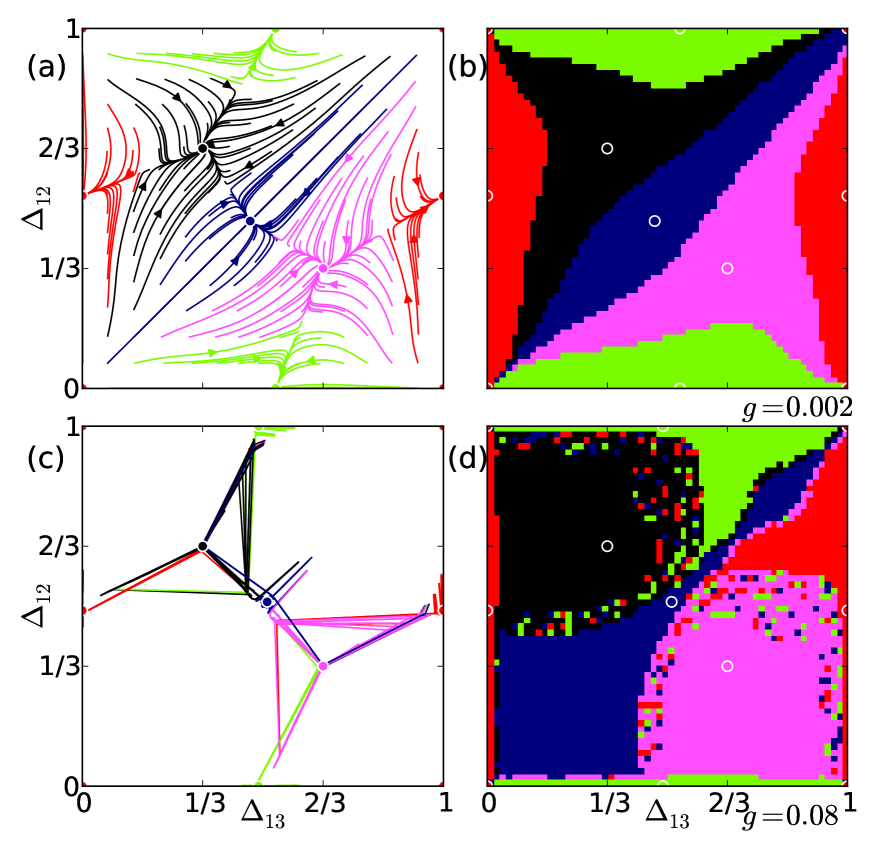
Figure 3: (Color online) Polyrhythmicity in the torus representation of phase lags. (a) At $g=0.002$, the return map reveals the underlying flow of phases converging to five stable FPs (circles). (b) By color-coding initial conditions according to the final rhythm, the basins are visualized. (c) At $g=0.08$, convergence in the return map is fast and no phase flow is discernible. (d) The structure of color-coded attraction basins reveals rigid boundaries. Parameters: $I=0.41$, $\varepsilon=0.15$.

II.4 Mapping Phase Basins

Return maps (Sec. II.3) allow us to partition the phase torus into attraction basins of the coexisting stable FPs. Numerically, we compute a basin as a finite set of initial conditions converging to a particular FP. The boundaries separating two neighboring basins are approximated by delineating adjacent initial conditions on the torus that result in two different rhythms.

To numerically determine these basins, we first create a grid of initial conditions densely covering the torus. We then attribute each point on the grid to a stable rhythm that establishes in the circuit after a transient. This method is illustrated in Fig. 3(b) showing the torus partitioned in the five color-coded attraction basins. For example, all initial states lying within the blue region converged to the pacemaker rhythm corresponding to the FP, $(\frac{1}{2},\frac{1}{2})$, which is located in the middle of the torus.

When coupling is weak, the basin approach does not add information to the knowledge deducted from return maps. For example, Figs. 3(a) and (b) disclose the basins equally well. This is no longer the case for stronger coupling, where the approach based on attraction basins becomes very handy. For example at $g=0.08$, the phase-basin representation shown in Fig. 3(d) offers more insight into the circuit dynamics than the return map shown in Fig. 3(c). Unlike maps for weak coupling, stronger coupling results in the faster convergence of $V$-traces and phase trajectories to corresponding stable FPs over the course of a few iterations. Therefore, the return-map method gives a good projection of circuit dynamics only when a slow-fast decomposition is possible. Herein, the strength of phase coupling governs the slow time scale, which however, is not small anymore in the circuit whose dynamics are depicted in Figs. 3(c) and (d). A good indication of this limitation is the fractal break-up of basin boundaries apparent in Fig. 3(d), and which is not observed if time scales are well separated.

II.5 Finite Stochastic Perturbations

Robustness of circuit rhythms to perturbations is probed by adding white noise to each $V$-equation of the circuit in the following way:

$$\dot{V}_{i}=V_{i}-V_{i}^{3}+I-x_{i}-g\sum_{i\neq j}G(V_{i},V_{j})+\sigma\xi_{i}(t)\leavevmode\nobreak\ ,$$ (4)

where $\langle\xi_{i}(t)\xi_{j}(t^{\prime})\rangle=\delta_{ij}\delta(t-t^{\prime})$ and $i,j=1,2,3$. Unlike the deterministic case, the stochastic dynamics show sudden transitions among multiple coexistent rhythms, which are stably generated by the circuit otherwise. Such switching is intensified at higher noise intensity $\sigma$, but foremostly depends on properties of the polyrhythm at given circuit parameters. Fig. 4(a) illustrates the evolution of a stochastic trajectory of the circuit that begins in the vicinity of $\Delta=\left(\frac{1}{2},\frac{1}{2}\right)$. The circuit mainly switches among the three coexistent pacemaker states, and sporadically transitions throughout the wave rhythms. This wandering of the phase lags is shown in the return map (Fig. 4(b)). The phase lags, taken modulo one, form clusters in the vicinity of pacemaker rhythms. The unwrapped phase lags, defined without modulo-one and shown in Fig. 4(b), allow us to characterize the two-dimensional random walk.

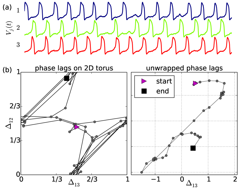
Figure 4: (Color online) Example of 2D phase diffusion in the stochastic circuit. (a) An excerpt of the example traces $V_{j}(t)$ shows erratic transitions between wave and pacemaker rhythms; color-coded bars indicate synaptic activation in the nodes. (b) Evolution of the corresponding phase lags (taken on modulo one and unwrapped by Eq. (5)) in a torus (left), and a phase plane (right) depicting a phase diffusion.

To evaluate the unwrapped phase lags, we use a more general definition of phase. As before, we employ return-time sequences $t_{j}^{(k)}$ for the oscillators (Sec. II.3). Then, define the unwrapped phase at each return time as follows $\varphi_{j}(t_{j}^{(k)})=k$. Next, phase differences, $\varphi_{j}(t)$ are defined in between two successive return times using linear interpolation ($t_{j}^{(k)}<t<t_{j}^{(k+1)}$) [42]:

$$\varphi_{j}(t)=\frac{(k+1)(t-t_{j}^{(k)})+k(t_{j}^{(k+1)}-t)}{t_{j}^{(k+1)}-t_{j}^{(k)}}\leavevmode\nobreak\ .$$ (5)

This phase differs from the previous definition [Eq. (2)] in two principal aspects: (i) the newly defined phase lets us monitor continuous unwrapped phase differences $\Delta_{1j}=\varphi_{1}-\varphi_{j}$, which cannot be recovered from the representation with modulo one. (ii) Through Eq. (2) we have phase lags normalized by the period of the reference node 1, whereas in Eq. (5), we normalize the phase of each oscillator with its individual period. By comparing two panels in Fig. 4 one can see that as long as the individual periods do not differ substantially, both definitions agree well on the torus.

Diffusion coefficient. The unwrapped phase lags perform a random walk. After many oscillations, the variance of each phase lag scales linearly in time: $\langle(\Delta_{1j}^{(n)})^{2}\rangle=D_{j}n$, wherein the proportionality constant $D_{j}$ is the diffusion coefficient. We compute the joint diffusion constant as a sum, $D=D_{2}+D_{3}$, because correlations between phase lags vanish in the symmetric circuit. The average is taken over representations of noise. To estimate $D_{j}$, we first compute a long phase trajectory $\Delta^{(n)}$. We divide the trajectory in segments of $50$ oscillations and compute the two variances $\langle(\Delta_{1j}^{(n)})^{2}\rangle$. Each diffusion coefficient is determined by a linear fit with respect to $n$, and then the two estimates are summed to obtain $D$.

Alternatively to perturbing $V$-variables, it is possible to add noise to the $x$-variables. While the diffusion motion at fixed values of $\sigma$ differs, the qualitative results of polyrhythmic robustness are comparable.

II.6 Standard Phase Reduction

A perturbation approach lets us derive phase equations for two phase-difference variables defined on the periodic orbit of the individual nodes [43]. These phase variables can be approximated by those introduced in Sec. II.3. The computation requires the uncoupled periodic orbits and their phase resetting curves, which we find with AUTO (Sec. II.7).

We map the uncoupled ($g=0$) periodic orbit $y(t)=(V(t),x(t))$ of period $T$ to a phase variable $\varphi(y)\in[0,1)$. The phase is required to increase constantly: $\dot{\varphi}=\omega=1/T$. The last assertion fixes the definition of $\varphi$ up to a constant phase shift. To quantify how coupling influences this phase, we compute the infinitesimal phase resetting curve $Q(\varphi)$ (PRC) for the $V(t)$-variable . Then, the phase variable $\varphi_{j}$ for node $j$ is given by ($i,j=1,2,3$)

$$\dot{\varphi_{j}}=\omega+gQ(\varphi_{j})\sum_{i\neq j}G(V_{j}(\varphi_{j})\leavevmode\nobreak\ ,V_{i}(\varphi_{i}))\leavevmode\nobreak\ .$$ (6)

This already reduces the number of equations from six to three. Below we will use a short notation $G(\varphi_{j},\varphi_{i})$ for $G(V_{j}(\varphi_{j}),V_{i}(\varphi_{i}))$.

For sufficiently small $g$, the phase equations [Eqs. (6)] hide a separation of time scales allowing for a further reduction to two variables. The separation becomes visible in Fig. 1 showing slow convergence to stable fixed points over the course of many oscillations. Therefore, we consider the phase differences, $\Delta=(\Delta_{12}=\varphi_{1}-\varphi_{2};\leavevmode\nobreak\ \Delta_{13}=\varphi_{1}-\varphi_{3})$. Their dynamics are of the order of the coupling strength $g$, which is slow compared to $\omega$:

$$\begin{aligned} \dot{\Delta}_{1j}&=gf_{1j}(\Delta;\varphi_{1})\leavevmode\nobreak\ ,\quad\text{where}\\ f_{1j}&=Q(\varphi_{1})\sum_{i\neq 1}G(\varphi_{1},\varphi_{i})-Q(\varphi_{j})\sum_{i\neq j}G(\varphi_{j},\varphi_{i}).\end{aligned}$$ (7)

Introducing $\varphi_{i}=\varphi_{1}-\Delta_{1i}$ for $i=2,3$, and integrating Eq.(7) over the fast variable $\varphi_{1}$ on $[0,1)$, we obtain

$$\begin{aligned} \dot{\Delta}_{1j}&=gf_{1j}(\Delta),\quad\text{where}\\ f_{1j}(\Delta)&=\int\limits_{0}^{1}f_{1j}(\Delta;\varphi)\leavevmode\nobreak\ d\varphi.\end{aligned}$$ (8)

This calculation gives us a direct access to the vector field $f_{1j}(\Delta)$ determining all fixed points of the circuit and their stability in the weak coupling limit. Moreover, the result depends on neither the choice of $\varphi_{1}$ as the reference phase, nor which phase variable is used for averaging.

II.7 Bifurcation Analysis and Continuation of Periodic Solutions

II.7.1 Stability of Periodic Orbits

The circuit dynamics [Eq. (1)] can also be analyzed with numeric parameter continuation if circuit rhythms are period orbits [45]. Essentially, one computes the stability multipliers corresponding to a Poincaré map of the orbit. Let us treat the circuit as a system of six ordinary differential equations $\dot{y}=f(y;p)$ with a vector $p$ of bifurcation parameters. An observable circuit rhythm is a stable $T$-periodic orbit, $y(t+T)=y(t)$, of this system. Formal linearizing the system on the orbit leads to the following variational equation

$$\dot{v}=A(t)v,\quad\text{where}\quad A(t)=Df(y(t);p)\leavevmode\nobreak\ ,$$ (9)

with a $6\times 6$ matrix $A(t)$ of periodic coefficients. This equation describes how infinitesimal deviations $\xi(0)$ from the periodic orbit may grow or decay as time progresses: $\xi(t)=\Psi(t)\,\xi(0)$; here $\Psi(t)$ is the fundamental matrix [41]. Its eigenvalues, $\lambda_{k}$ ($k=0,\dots,5)$, are called the Floquet multipliers. For each $\lambda_{k}$, there is an eigenvector $v_{k}(t)$ with the property $v_{k}(T)=\lambda_{k}v_{k}(0)$. In other words, the multiplier $\lambda_{k}$ quantifies the growth rate of a perturbation from the periodic orbit in the direction $v_{k}$ after a single evolution of the circuit rhythm.

Each orbit always has one multiplier, say $\lambda_{0}$, equal to $+1$. It corresponds to perturbations along the orbit, which neither increase nor decrease on average over the period $T$. If all other multipliers fulfill the condition $|\lambda_{k}|<1$, then the periodic orbit is Lyapunov stable. The values of three multipliers, say $\lambda_{3}$, $\lambda_{4}$, and $\lambda_{5}$, are close to zero at the coupling strength considered here. They correspond to strongly stable directions towards the stable periodic orbits in the individual nodes. These directions are perpendicular to those determined by the vector tangent to the periodic orbit, and hence to those on which the phase lags are defined on the periodic orbit. The remaining two multipliers, $\lambda_{1}$ and $\lambda_{2}$, correspond to perturbations parallel to the phase lags. These multipliers govern the stability of circuit rhythms, and are therefore called control multipliers below.

We say that a bifurcation in the circuit occurs when one, or both, multipliers $\lambda_{1,2}$ cross a unit circle outward, i.e $|\lambda_{k}|=1$, as circuit parameters are varied. This bifurcation gives rise to the stability loss of a circuit rhythm though a pitchfork or a flip (period doubling) bifurcation, or the disappearance of the stable rhythm through a generic saddle-node bifurcation. The case where a pair of complex conjugate multipliers $\lambda_{1,2}$ leaves a unit circle corresponds to a torus or a secondary Andronov-Hopf bifurcation. This bifurcation can give rise to the emergence of a stable invariant circle in the Poincaré return map. Such a stable circle is attributed to the onset of phase jiggling in the voltage traces [12, 35]. The jiggle frequency is determined by the angle $\theta$ of the multipliers, i.e. $\lambda_{1}=e^{\pm i\theta}$. Moreover, if $\theta$ is a simple multiple of $\pi$, the torus bifurcation unfolding becomes more complex because of the occurrence of strong resonances at $\theta=\pi$, $\frac{2\pi}{3}$, and $\frac{\pi}{4}$ [41].

II.7.2 Numerical Computation

The bifurcation analysis of periodic orbits in the circuit was carried out with use of parameter continuation package AUTO-07p [46]. Specifically, we set up Eqs. (1) in AUTO to investigate the stability of the wave and pacemaker rhythms under the variation of parameters $\varepsilon$, $I$, and $g$.

In our simulations, AUTO was initially used to compute the stable periodic orbit (PO) and phase resetting curves (PRCs) for each individual oscillator. Before, an uncoupled oscillator ($g=0$) was numerically integrated until a transient relaxed onto the PO, and an individual oscillation was recorded. The data was used as an initial guess for AUTO to approximate the PO as precisely as possible. By simultaneously solving the adjoint equation, we also obtained the PRC describing perturbations of the $V$-variable.

Next, AUTO was employed to investigate POs in the full, coupled circuit, to examine their dependence on the control parameters $I$, $g$, and $\varepsilon$. We first found an initial guess for the circuit PO at parameter values $I=0.51$, $\varepsilon=0.3$, and $g=0.01$. At these values, the two coexisting wave-rhythm POs of the circuit are pre-dominantly stable and can be easily detected. We then continued either solution in the parameters $I$, $\varepsilon$, and $g$ to examine its bifurcations, as well as to monitor quantitative variations in the Floquet multipliers of the circuit PO. This allowed us to detect bifurcations and changes in stability. Similarly, we also investigated properties of the three symmetric pacemaker rhythms dominating the dynamics of the circuit at $I=0.41$. Below we analyze in detail the bifurcation boundaries demarcating the stability and existence regions of the circuit polyrhythm.

We performed all of our computations with Motiftoolbox, an in-house developed simulation package that combines powerful computation software libraries such as Compute Unified Device Architecture, GNU Scientific Library, python-scipy, python-matplotlib, and AUTO-07p. .

III Results

III.1 Qualitative Stability of Polyrhythms

III.1.1 Phase Analysis of Polyrhythmicity

The three-node circuit [Eq. (1)] exhibits up to five stable rhythms, for example at the parameter values $I=0.41$, $g=0.08$, and $\varepsilon=0.15$, as shown in Fig. 3. Two rhythms are of the wave type and three are of the pacemaker type. While these numbers are formally due to permutation symmetries of the circuit [48, 49], the question of whether the given rhythm exists and is stable or unstable solely depends on the parameters of the circuit [35].

Return-map analysis. We investigated the stability of the rhythms for a broad range of circuits by systematically varying the three parameters $I$, $g$, and $\varepsilon$. For every point in a grid of this parameter space, we identified all stable rhythms by analyzing the phase dynamics of the circuit, as shown in Fig. 3. We examined the following parameter ranges of $\varepsilon\in[0.1,0.3]$, $g\in[0.001,0.1]$, and $I\in[0.4,0.6]$ to span dynamical scenarios of slow-fast versus normal time scales, weakly versus strongly coupled circuits, and release versus escape mechanisms of node dynamics, respectively.

We found regions in the three-dimensional parameter space where either wave, pacemaker, or both rhythms are stable. This is illustrated in Fig. 5, where we show four parameter sweeps in $g$ and $I$, each one with a different value of $\varepsilon$.

As evident in the figure, we find that the Pacemaker rhythms are stable in a vicinity of the release and escape case, for which $I\approx 0.4$, and $I\approx 0.6$, respectively. The region of instability, enclosed by solid black lines, did not seem to depend on $\varepsilon$.

On the contrary, stability regions of wave rhythms depend on $\varepsilon$. At values of $\varepsilon<0.1$, at which time scales are well-separated, the wave rhythms are stable in the whole parameter space. At $\varepsilon$ larger than $0.11$, regions in parameter space form in which wave patterns are unstable. The dependence is visible in Fig. 5(c) at $\varepsilon=0.13$, where a region of wave instability becomes visible at $g>0.08$ and $I\approx 0.45$. The region grows with $\varepsilon$ and then merges with another region emerging from the release border at $I=0.4$.

We analytically determined the hard-lock transition of inhibitory coupling (dashed-dotted [pink] lines in Fig. 5), beyond which one, active oscillator is able to lock down another oscillator at a stable inactive state. Because active phases in wave rhythms tend to overlap in time, the mechanism could influence the stability of these rhythms. Indeed, we found at large values of $\varepsilon$, that the boundary of wave stability correlates well with the hard-lock transition of coupling strength, for example at $\varepsilon=0.17$ shown in Fig. 5(a). At smaller values of $\varepsilon$ we did not find such good correspondence.

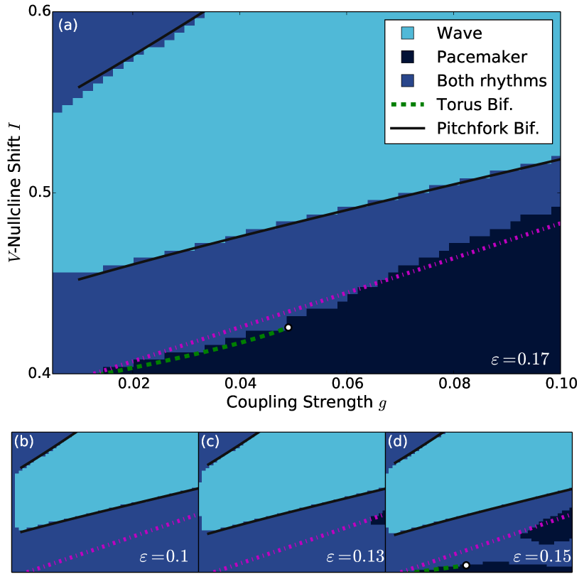
Figure 5: (Color online) Qualitative stability of circuit polyrhythms in three parameters. For a grid of $I$, $g$ and $\varepsilon$, we determine the stability of wave and pacemaker rhythms using the phase-basin method (Sec. II.4 and Fig. 3(b),(d)). Each plot (a)-(d) shows a bi-parametric sweep in $I$ and $g$ at fixed $\varepsilon$ as indicated. The regions of stability for wave (light blue), and pacemaker rhythms (navy) can be distinct, or show an overlap (dark blue), at which both rhythms are stable. Pure pacemaker regions at low $I<0.5$ and large $\varepsilon>0.15$ correlate with the soft-to-hard lock transition (dashed dotted line). Region borders indicate bifurcations where one rhythm becomes unstable. Bifurcation lines of a pitchfork and a torus bifurcation (Bif.) were determined with AUTO.

Standard phase reduction. Return-map analysis is impractical at weak coupling because convergence of transients to stable rhythms become very long. To analyze the stability of polyrhythms in this weak-coupling case, we used the methods of standard phase reduction (Sec. II.6).

We computed phase resetting curves (PRC) for a dense grid of parameters $I\in[0.4,\,0.6]$ and $\varepsilon\in[0.1,\,0.3]$. From these PRCs, we constructed the flow for the phase differences on a torus (Eq. (8)). We identify all equilibria of this flow. Applying the numerical differentiation tools, we can also assess the Lyapunov characteristic exponents of the equilibria. Our findings are documented in Fig. 6(a) representing the bifurcation digram in the ($\varepsilon,I$)-parameter plane of the weakly coupled circuit.

We find that pacemaker rhythms show a region of stability for values of $I$ close to release and escape, while enclosing a region where only wave rhythms are stable. This is in line with our results from the return map analysis (cf. Fig. 5). The boundaries of the pacemaker region weakly depend on $\varepsilon$, such that the region shrinks as $\varepsilon$ increases. We note that wave rhythms always coexist for the range of parameter values in $\varepsilon$ and $I$ considered in Fig. 5. Nevertheless, at larger values of $\varepsilon\geq 0.23$, a region emerges in which the wave rhythms becomes unstable, and pacemaker rhythms are the only stable attractors. Compared to moderate values of coupling, the regions found here are very thinly around the release and escape case.

Figure 6: (Color online) Polyrhythms stability in the weak-coupling limit. For a grid of $I$ and $\varepsilon$, we determine the stability of wave and pacemaker rhythms using the standard phase reduction (Sec. II.6). (a) a bi-parametric sweep in $I$ and $\varepsilon$ for infinitesimal $g$. The regions of stability for wave (light blue), and pacemaker rhythms (navy) can be distinct, or show an overlap (dark blue), at which both rhythms are stable. Region borders indicate bifurcations where one rhythm becomes unstable. A torus bifurcation (Bif.) was determined. (b) The imaginary part of the wave rhythm’s Lyapunov exponent is color-coded. The exponent is imaginary at the border of wave instability indicating a torus bifurcation (green dashed line).

The phase-reduced circuit dynamics (summarized in Fig. 6) are primarily determined by the coupling function $G(V_{i},V_{j})$ and the phase resetting curve (PRC) $Q(\varphi)$ given by Eq. (6). As $G$ does not depend on the parameters, differences in PRCs are responsible for the variations in circuit dynamics shown in Fig. 6. We computed PRCs for a series of parameters $I$ and $\varepsilon$ to understand how the different patterns of polyrhythmicity relate to these fundamental functions.

Six representative PRCs are shown in Fig. 7 for the escape case in Panels (a, b); for the centered nullclines in Panels (c, d); and for the release case in Panels (e, f), at two different values of the time-scale parameter $\varepsilon=0.1$ and $0.25$. Each curve was characterized by a negative and a positive inflection, or bump. These inflections appeared in each of the phase-parameterized stagnation regions at the lower and upper fold of the $V$-nullcline. The upper stagnation region appeared first in the PRC. The associated negative inflection indicates that a perturbation with positive sign causes a phase delay, thus prolonging the active state. The opposite is true for the latter, positive inflection that was located at the lower stagnation region. Note also that the PRC amplitudes are arbitrary because the phase theory is taken to a linear order only. Parameter $I$ affected PRCs in two ways: increasing $I$ shifted the first inflection to later phases. It also rebalances the inflection amplitudes towards the first one. The time-scale parameter $\varepsilon$, on the other hand, affects the width of the inflections.

Figure 7: (Color online) Phase resetting curves of activity variable. The infinitesimal phase resetting curve is tabulated for values of $I$ and $\varepsilon$ (indicated). Values for $I$ correspond to (a, b) escape- ($I=0.6$), (c, d) normal- ($I=0.5$), and (e, f) release- ($I=0.4$) cases, which are shown for separate and similar time scales, at $\varepsilon=0.1$ and $\varepsilon=0.25$, respectively. Note that amplitudes of infinitesimal PRCs are unit-free because perturbations are linearized.

III.1.2 Bifurcation Analysis of Circuit Rhythms

We investigated the dynamical scenarios through which circuit rhythms loose or gain stability at the region borders shown in Fig. 5. Such bifurcations for the wave and pacemaker rhythms, respectively, were visible in return maps for small enough values of coupling strength, $g$. It was also possible to characterize some of the bifurcations with AUTO.

Pacemaker rhythms. Our analysis of return maps revealed that every pacemaker rhythm first loses, and then gains stability back through a pitchfork bifurcation as the parameter $I$ is increased from $0.4$ through $0.6$. At the pitchfork bifurcation a stable fixed point (corresponding to either pacemaker) becomes unstable after it merges with two nearby saddle fixed points to become a saddle itself, that next becomes stable again through a reverse bifurcation. Such a bifurcation sequence was clearly visible in the maps for small $g$, as exemplified in Fig. 8.

We used AUTO to trace the bifurcation in two parameters with high accuracy. For this, we initialized one of the pacemaker rhythms as a periodic orbit at $I=0.41$. The results do not depend on the choice of rhythm because symmetry ensures that all pacemaker rhythms have the same stability properties. We found the numerically precise parameters of the bifurcations by increasing $I$ at fixed $\varepsilon$ and $g$ when the control Floquet multiplier of the orbit becomes $+1$. We then continued the bifurcation in $I$ and $g$ through the entire parameter range (black lines in Fig. 5). The procedure was repeated for each $\varepsilon$. We found that the bifurcation curves precisely correspond to the region borders found in return maps.

Figure 8: (Color online) Pitchfork bifurcation of a pacemaker rhythm. When $I$ increases from (a) $0.43$ to (b) $0.46$, the pacemaker rhythms undergo a pitchfork bifurcation, here shown for a part of the full torus (Fig. 3). Two saddles (black squares) collide with the fixed point corresponding to the blue pacemaker rhythm (circle in the center). Beyond $I=0.46$, only the two wave rhythms (circles in upper-left, and lower-right corners) are stable. Parameters: $\varepsilon=0.17$, and $g=0.01$.

Wave rhythms. We found the bifurcation of wave rhythms to be more complex. Along the border of instability (blue and dark-blue region in Fig. 5(a)), the bifurcation changed its type from torus bifurcation at small $g$, to saddle-node bifurcation involving three saddles at larger $g$.

At small $g$, the bifurcation type was discernible in return maps as documented in Fig. 9. Decreasing $I$ at low values of $g$, we found a torus bifurcation leading to an invariant cycle (Fig. 9(a)). The circle grew in size with further decreases of $I$ until it became a heteroclinic orbit connecting three saddle fixed points. The heteroclinic bifurcation completed the sequence: once the heteroclinic connection broke down, the pacemaker rhythms dominated the dynamics of the circuit.

Figure 9: (Color online) Destabilization of the wave rhythms. At $\varepsilon=0.3$, When we decrease $I$ from $0.415$ to $0.4$ the wave rhythms located at $\Delta=(2/3,1/3)$ loses stability. At values $I>0.415$, the basin of attraction of the wave rhythm persistently shrinks. Around $I=0.41$, a torus bifurcation gives birth to a stable invariant cycle, through which the wave rhythm also loses stability. The invariant cycle grows until it merges with three saddles (black diamonds) in a heteroclinic bifurcation around $I=0.406$. After the heteroclinic bifurcation, the former wave basin is divided among the pacemaker rhythms.

By performing AUTO simulations we could accurately detect the torus bifurcation in the diagram. As before, we initiated the circuit on either stable wave rhythm at $I=0.4$. The corresponding periodic orbit was then numerically continued by varying $I$ at fixed $\varepsilon$ and $g$ until AUTO detected the torus bifurcation. Next, the torus bifurcation was parametrically continued in $I$ and $g$, thus tracing down the bifurcation curve represented by dashed lines in the diagram shown in Fig. 5. The found segment of the corresponding bifurcation curve is located in proximity of the associated region border found through the return maps. We were not able to detect or continue the heteroclinic bifurcation.

Despite all efforts, we were also unable to continue the torus-bifurcation curve for values $g$ greater than $0.05$ when using AUTO. To find out the cause of its malfunction, we examine the behavior of the pair of complex-conjugate Floquet multipliers, $e^{\pm i\theta}$, corresponding to the torus bifurcation. Given that $||e^{\pm i\theta}||=1$ at the bifurcation, we assessed the angle, $\theta=|\arg e^{\pm i\theta}|$, as a function of $g$. In the uncoupled case, the angle is zero because all phase lags are constant. We found that for increasing $g$ the angle grows monotonically until it reaches $\pi$, as illustrated in Fig. 10 for $\varepsilon=0.17$. We also detected the values of $g$ at which the angle reaches strong resonances. Of special interest to us is the $\frac{2\pi}{3}$-strong resonance. In theory this resonance gives rise to the emergence of a resonant invariant circle (torus) containing a saddle-node orbit of period three [41]. It is known too that the bifurcation unfolding of the $\frac{2\pi}{3}$-resonance case involves a further bifurcation resulting in that three saddle fixed points collapse into the bifurcating one making it a saddle with six separatrices. Studies of such codimension-two bifurcations are the state of the art that no simulation package can handle.

Figure 10: (Color online) Bifurcation scenario of the wave rhythm. The wave rhythm’s complex-conjugate Floquet multipliers $\mu=\text{e}^{i\theta}$ at the torus bifurcation change their critical angle $\theta$ along the bifurcation curve (inset). The angle $\theta$, grows with increasing coupling strength $g$. It passes resonances $\pi/2$ and $3\pi/2$ after which $\theta$ approaches $\pi$. The angle decreases to zero when extrapolated to $g=0$ (dashed-line). Parameters: $\varepsilon=0.15$ and $I(g)$ as shown in Fig. 5(d).

III.2 Quantitative Stability of Polyrhythms

We assess quantitative stability of the circuit rhythms by applying infinitesimal and finite stochastic perturbations. Infinitesimal perturbations do not induce switching from rhythm to rhythm; instead, they offer insight into the local stability of wave and pacemaker rhythms separately. Finite perturbations induce switching, and therefore inform about the stability of the polyrhythm, which we also call robustness.

III.2.1 Linear and Local Stability

The standard phase reduction method (Sec. II.6) approximates the phase dynamics as follows: $\dot{\Delta}=gf(\Delta),$ ($\Delta=(\Delta_{12},\Delta_{13})$) The stability of an equilibrium state $\Delta^{\ast}$ is determined by the eigenvalues $\lambda_{1,2}$ of the differential $Df(\Delta^{\ast})$. It is exponentially stable if $|\lambda_{1,2}|<0$. Coupling strength $g$ scales the exponent values proportionally: increasing $g$ enhances the stability of a stable rhythm, while pronouncing the instability of an unstable one.

We counterpose this assertion with the exact calculation of the leading Floquet exponent $\mu$ using AUTO (Sec. II.7). For weak coupling, $\mu$ is equivalent to the leading eigenvalue $\lambda$ evaluated through phase reduction.

For a grid of parameter values $I$, $g$ and $\varepsilon$, we computed the leading Floquet exponent $\mu$ for the traveling wave and a pacemaker rhythm. Note that all permutation-symmetric rhythms have the same set of exponents [48, 49]. The corresponding bifurcation diagrams for $\varepsilon=0.17$ are shown in Fig. 11 (cf. Fig. 5(a)). The exponents changed signs exactly at the pitchfork and torus bifurcations for the pacemaker and wave rhythms, respectively. For weak coupling strength $g$, the exponent $\mu$ shows a monotonous dependence on $g$, which breaks down in a vicinity of the bifurcations. Strengthening $g$ for the wave rhythm revealed a parabola-shaped set of minimal values of $\mu$ in the bifurcation diagram. At these parameter values, the local linear stability of wave rhythms reached its maximum. At low values of $I$, the wave rhythms become highly unstable.

Figure 11: (Color online) Leading Floquet exponent of circuit rhythms. The largest, non-zero Floquet exponent determines the linear stability of the (a) pacemaker and (b) wave rhythms. The values, indicating stability ($\mu<0$) or instability ($\mu>0$) of the rhythms, are proportional to $g$ at weak coupling, unless in the vicinity of bifurcations (black-solid, and green-dashed lines). The wave rhythms are the most stable on a parabola-shaped set in the $(g,I)$-parameter plane, and highly unstable at low values of $I$.

III.2.2 Robustness of Polyrhythmicity

We tested the robustness of polyrhythmic circuit dynamics under noisy perturbations. Robustness was quantified by the phase diffusion constant for the phase-lag variables described in Sec. III.2.2. We found that the diffusion constant varies by orders of magnitude across the tested parameter space of $I$, $g$, and $\varepsilon$. Therefore, we carefully selected a value of noise intensity $\sigma$ that allowed us to sample the wide range of parameters with comparable accuracy. At small $\sigma$, noise caused only few switching events within $20000$ circuit-rhythm periods, and therefore no feasible estimation for $D$ was possible. We therefore present our results for $\sigma=0.01$, below. The value, $\sigma=0.02$, yielded similar results.

In the region where waves are the only stable rhythms, the phase diffusion constant showed a monotonous dependence on all parameters (cf. Fig. 12 between the solid black lines). Outside this region, the parameter dependence of $D$ shows considerable complexity. In Fig. 13, we supplement our findings with exemplary traces of the circuit dynamics.

Close to the escape case, the phase diffusion constant $D(I)$ at fixed $g$ and $\varepsilon$ shows a series of minima and maxima. A comparison with the deterministic bifurcation diagram (Fig. 5) revealed that the minima of $D$ somewhat align with both, the soft-to-hard lock transition line and the wave-instability line at $\varepsilon>0.13$. However, this is not the case at $\varepsilon=0.1$ where the wave rhythm did not bifurcate, while $D$ still showed a pronounced valley of stable dynamics (cf. Fig. 13(1),(2)).

The diffusion constant $D$ becomes increasingly large as $I$ approaches the boundary $0.4$ for all values of $g$ and $\varepsilon$. This is related to the highly vulnerable dynamics of the individual oscillators near the saddle-node bifurcation.

Figure 12: (color online) Phase diffusion constant $D$ of stochastic circuit dynamics. Random perturbations induce rhythm switching in the circuit, resulting in a finite phase diffusion constant $D$. Where the circuit demonstrates only wave rhythms (between black lines), $D$ depends weakly on $I$, $g$, and $\varepsilon$. Elsewhere, the dependence is complex and cannot be explained by the local bifurcation structures in the coexistence region of all five polyrhythms. $\sigma=0.01$.

IV Discussion

Previous studies have demonstrated that mutually inhibitory three-node circuits of neuronal bursters synchronize in up to five coexistent stable rhythms [12, 35, 37]. Out of these five, three are pacemaker rhythms, and two are the clockwise and counterclockwise wave rhythms. Disturbances with external current pulses or noise can cause switching among the rhythms. To better understand mechanisms of stability and robustness of polyrhythmicity, we have explored in this paper circuit dynamics constituted by generic relaxation oscillations. We set out to explore a wide parameter range to catalogue and describe the circuit dynamics in its entirety.

In particular, we investigated the circuit dynamics [Eq. (1)] depending on three principle parameters: the time-scale separation $\varepsilon$ determines the speed of the recovery variable $x$ with respect to the activity variable $V$ in each node; parameter $I$ shifts the position of the $V$-nullcline and thus controls the release and escape mechanism (cf. Fig. 2(b),(c)); and the inhibitory coupling strength $g$ determines how strong the node dynamics are tied to each other in the circuit. Here, we also distinguished a hard-lock coupling regime where inhibition is strong enough to fix the inhibited node in the inactive state.

We used in our circuit a Fitzhugh-Nagumo model with an $x$-nullcline, $x_{\infty}(V)$, that shows a sigmoidal shape and thereby deviates from the standard linear function. This choice is relevant especially for biological applications: it closely resembles corresponding Boltzmann and Hill functions that appear in Hodgkin-Huxley-type neuronal dynamics and enzyme kinetics, for example. Moreover, our choice allowed us to study transitions in the circuit dynamics related to the release and escape mechanisms, which are fundamental mechanisms of rhythmogenesis.

IV.1 Qualitative Stability of Polyrhythms

Circuit dynamics were particularly sensitive to the $V$-nullcline shift $I$ when set close to the release or escape case (Fig. 2(b),(c)). In both cases, the dynamics of individual oscillators are close to a saddle-node (SN) bifurcation emerging around the lower or upper fold of the $V$-nullcline, respectively. Such SN ghosts are known to substantially reduce the individual oscillation frequencies. Our results show that the two mechanisms qualitatively affect the circuit dynamics through interactions with inhibitory coupling, as described further below.

Let us first discuss the generic case of intermediate $I$-values. Here, individual oscillators are not close to any bifurcations, and we observed wave rhythms as the only stable circuit dynamics (cf. Fig. 5). The inhibition exerted by an individual oscillator is not strong enough to overcome mutual phase repulsion of the other two oscillators. Conversely, the pacemaker rhythms were unstable in this region.

Release case. At low values of $I$, corresponding to the release case, inhibitory coupling has a drastic effect on the dynamics of the inhibited nodes, specifically in the region of stagnation at the lower fold. Weak inhibition brings the dynamics of individual oscillators closer to the SN bifurcation at the lower fold; inhibition where the coupling parameter is larger than $g_{\rm crit}$ induces a transient SN bifurcation, leading to a stable equilibrium state [37]. With such strong inhibition, one oscillator locks down the other oscillators in the inactive state for the time it is active. As a result, the distribution of phases along individual orbits is highly non-uniform, and condensed around the stagnation region: each oscillator is either in a short active state, or it stagnates near the SN equilibrium. Naturally, two of the three oscillators must collapse in one of these two states, and thus synchronize. According to this description of two quasi-discrete states, the three-state wave rhythms are very unstable. Evidence for this heuristic description is the close proximity of the border of wave stability (border of blue to navy region in Fig. 5(a)) and the hard-lock transition line (magenta dashed-dotted line), that was visible at $\varepsilon=0.17$. For smaller values of $\varepsilon$ however, i.e. at large time-scale separation, we did not observe this mechanism (cf. Fig. 5(b) where $\varepsilon=0.1$). At these values, the slow dynamics of the recovery variable spreads active and inactive states along the branches of the slow manifold. Therefore, the heuristic description is not valid in this case.

Escape case. When increasing $I$ towards the escape case, we again found a region of parameter space wherein pacemaker rhythms are stable. As shown in Fig. 5, the effect did not depend on $\varepsilon$ and was most pronounced at small coupling strengths, which we also confirmed in the weak-coupling limit (Fig. 6(a)). The SN ghost, here located at the upper fold (Fig. 2(c)), plays a key role in the emergence of pacemaker rhythms. Analogous to the release case, the upper fold forms a stagnation region that leads to a highly non-uniform distribution of phases. Consider oscillators 1 and 2, that are in active states. The states approach each other as they slow down in the vicinity of the stagnation region. When the third oscillator becomes active, its inhibition breaks stagnation by widening the gap between $V$- and $x$-nullcline. Thus, oscillators 1 and 2 can simultaneously “escape” from the ghost and synchronize in a pacemaker rhythm. With only this mechanism, the pacemaker region should extend to higher coupling strengths, which is not the case (cf. Fig. 5). The mutual interaction of the oscillators 1 and 2, in the example, prevents their synchronization for strong coupling: if they strongly inhibit each other in the stagnation region, the oscillator 1 slightly lagging behind will repress oscillator 2 and push it through the stagnation region into the inactive state. In effect, oscillator 2 will cease to inhibit oscillator 1 which, thus, lingers on in the stagnation region. This explains our observation that the pacemaker rhythm was unstable.

The results for the release case are in line with those of Wojcik et al. [12]. In their model of neuronal bursting, which closely resembles the neuronal electrophysiology, a shift of a K⁺-conductance parameter induces the same series of bifurcations of the wave rhythms as those shown in Fig. 9. A dynamical analysis revealed that the shift widens the gap between the slow and fast nullclines at the lower fold [37], thus completing the analogy of the two observations. On the contrary, the escape mechanism is not observed due to inhibitory interactions of spikes [21]. In these parameter regimes, the burster models show different circuit dynamics compared with our relaxation oscillator.

IV.2 Quantitative Stability of Polyrhythms

Functional circuits often operate in environments where perturbations and noise interrupt their dynamics. In polyrhythmic circuits, this can lead to switching between coexistent rhythms and the switching process strongly depends on the circuit parameters. To analyze how robustly the circuit sustains a rhythm in such an environment, we randomly perturbed the circuit dynamics and monitored how individual phases diffused apart in consecutive random switching events. We found that the phase diffusion constant, indicating robustness of the polyrhythm, strongly depended on circuit parameters. However, we were unable to predict robustness by the bifurcation structure in the circuit or by linear-stability measures of individual circuit rhythms. One may still speculate why certain circuit configurations are more robust than others based on these information, for which we give two examples below.

In the wave-rhythm regions in Fig. 12, the dependence of $D$ on parameters $I$, $g$, and $\varepsilon$ is the most homogeneous. Strengthening inhibition, by increasing $g$, generally increases the local robustness of polyrhythms against noise as explainable in the linear stability theory (Sec. III.2.1). However, we find a vastly complex behavior in the region close to the release case (Fig. 13(a, b)). At small $\varepsilon$, a strip of stable wave rhythmicity is observed (Fig. 13(c)). By shifting $I$ to larger values, the robustness of the circuit becomes less pronounced. In this region, linear theory predicts pacemaker rhythms to be more stable (Fig. 11(a)). We speculate that increased stability of pacemaker rhythms facilitate switching, because they can better serve as intermediates in the switching process (Fig. 13(d)).

Generally, robust pacemaker rhythms can be achieved at larger values of $\varepsilon$, where the wave rhythms are less stable. At $I=0.48$, $g=0.09$, and $\varepsilon=0.17$, for example, all five rhythms coexist, but the wave rhythm is close to its stability boundary (cf. Fig. 5(a)). Here, pacemaker rhythms were commonly observed in randomly perturbed traces of circuit dynamics, as shown Fig. 13(e). One might expect to enhance stability of pacemaker rhythms by further reducing $I$ below the stability boundary of the wave rhythms. However, the circuit dynamics closer to the release case turns out to be highly vulnerable, especially below the hard-lock transition (dashed-dotted [pink] line). In this region, switching caused by noise among the three coexisting pacemaker rhythms becomes very frequent (cf. Fig. 13(f)). The increased intensity of switching is analogous to the observations in three-cell motifs of the Hodgkin-Huxley type bursters in Ref. [37], that demonstrated even weak noise can disrupt the pacemaker rhythms subjected to the hard-lock inhibition occurring in the release case.

Figure 13: (Color online) Stochastic circuit dynamics at different levels of robustness. The examples illustrate specific regions of interest in the complex rhythm robustness of stochastic circuit dynamics. Colors (gray scales) in Panels (a) and (b) are coded according to Fig. 12.

The closer the circuit is set to the release case (lower $I$), the higher the diffusion rate, $D$, becomes in the two-dimensional plane of phase differences.

IV.3 Comparison of Methods for Stability Analysis

We used several methods to carry out the qualitative and quantitative stability analysis of the circuit polyrhythms. The qualitative stability was assessed by standard phase reduction, phase mappings, phase-basin analysis, and direct bifurcation continuation. The quantitative stability was assessed by local methods of stability analysis derived from standard phase reduction, and the Floquet exponents of continued periodic orbits. It was also counterposed to random perturbation analysis in its effect on phase diffusion.

Qualitative Methods. Geometric and symmetry arguments in an all-to-all coupled circuit of oscillators grants the existence of periodic orbits [48, 50, 50, 51, 49]. However, these arguments cannot be applied to show whether the corresponding rhythms (orbits) are stable or not. Methods of automatic bifurcation analysis can answer this question successfully as demonstrated in this study (cf. Fig. 5). The approach fails, however, if circuit rhythms bifurcate. In the example of the wave rhythm, a torus bifurcation leaves the associated periodic orbit unstable; disregarding the resulting low-amplitude jiggle, the wave rhythm is still intact. In the example, the torus-bifurcation line (green dashed line in Fig. 5(a)) still coincides well with the border of wave instability, but only by the coincidence that the torus is stable for a small range of parameters. In such cases, the methods of phase description, such as return maps, are able to qualify that the torus orbit is still close to the wave rhythm (cf. Fig. 9(c)).

The phase approach is applied with three different methods in this work. In the weak coupling approximation, the standard method of phase reduction describes phase perturbations of individual periodic orbits by the phase resetting curve (PRC) to linear order. The method has many numerical advantages. The PRC is obtained by only regarding an individual oscillator; subsequently it can be used to explore the phase dynamics of arbitrarily large networks. Moreover, a high precision can be reached because the method does not require forward integration of the full circuit dynamics. One can therefore compute fixed points, as well as their eigenvalues of the phase flow, as demonstrated in Fig. 6.

As coupling is strengthened, the standard phase reduction fails to produce correct results because the individual periodic orbits become increasingly distorted by the inhibitory coupling. However, in principle, the phase dynamics remain slow compared to that for the amplitudes. Therefore, one can still compute the return maps from first return times of individual oscillations to reconstruct the phase flow. The distance between consecutive phase lags in the mapping will increase with stronger coupling because the phase dynamics become fast compared to the oscillation period. Eventually, phase trajectories are not discernible anymore and the phase-mappings method will fail.

Nevertheless, when phases jump erratically, it is still possible to re-construct some practical aspects of the phase dynamics, for example, the basins of attraction and their boundaries. In the brute-force scheme, the initial conditions can only form a topological equivalent of the individual periodic orbit. Therefore, the geometry of the basins is strongly distorted. For example, the basins of the pacemaker rhythms may not appear equally sized, even though they are in this symmetric circuit (cf. Fig. 3(d)).

Quantitative Methods. Harder than the stability or instability of a circuit rhythm is the evaluation how stable a rhythm is. We used two approaches, in this work, to quantify stability depending on the assumed disturbances to the circuit dynamics: approaches of linear stability measure the effect of infinitesimal perturbations, whereas approaches with finite perturbations such as noise investigate the full polyrhythmic stability, or robustness.

Infinitesimal perturbations cannot excite the circuit to switch from a stable rhythm to another. Therefore, the wave and pacemaker rhythms have to be regarded separately. From such an element-wise description of polyrhythmicity, it is hard to predict the outcome of the switching behavior through Kramer’s rates, for example. This would only be possible if one were able to quantify a height of an assumed potential barrier separating stable circuit rhythms. Phase diffusion coefficients of noise-perturbed circuit dynamics, on the other hand, quantify random transitions between stable circuit rhythms. This measure is typically dominated by the most stable circuit rhythms, as highlighted in the examples in Fig. 13. The least stable rhythms take the role of unstable saddles at finite noise strengths, but may also serve as facilitating intermediates.

V Conclusions

Small circuits of inhibitory relaxation oscillators appear in many natural systems in order to flexibly generate rhythmic patterns of activity phases. In this article, we applied several computational methods to gain global understanding of the dynamical transitions in a circuit of three mutually inhibitory relaxation oscillators. We find that the two wave and three pacemaker rhythms, predicted to coexist in the circuit due to permutation symmetry, strongly depend on quantitative and qualitative features of the node dynamics and inhibitory coupling.

As a generic model of relaxation oscillations, we adopted a Fitzhugh-Nagumo-like system that exhibits two saddle-node bifurcations, beyond which oscillations stall. One bifurcation inactivates the oscillators, while the other stabilizes its active state. These dynamical regimes are non-generic for oscillators, but occur often in natural systems to facilitate flexible control of frequency and rhythmicity. Comparison of our results using the generic model and those of Wojcik et al. [12] and Jalil et al. [21] highlight to what extent the generic model can approximate Hodgkin-Huxley type bursting models. While the release case is well represented [12], the two models differ in the escape case where spikes play an active role in rhythmogenesis [21].

In our investigations, we find that closeness to bifurcations of individual oscillators has a profound effect on the dynamics of the whole circuit: a generic inhibitory circuit produces the wave rhythms, but close to the inactivating bifurcation, we find that the wave rhythms can become unstable to give room for pacemaker rhythms. We find the same dynamical instabilities in the case of strong inhibition. Past the hard-lock transition, all active phases of mutually inhibitory neurons need to be non-overlapping. This is possible in our three-node circuit where, conversely, wave rhythms may still be observed. However, for circuits consisting of more nodes, waves can become unstable due to such a crowding effect.

The method of phase basins described in this article gives a natural extension to the return maps of Wojcik et al. [12], that allows for the treatment of strong coupling in polyrhythmic circuits. Tracking phase basins across coupling strengths allows us to identify bifurcations that can be utilized for the control of rhythms in the circuit. Such coupling control may be of particular experimental relevance in neuroscience, because inhibitory synaptic strengths are easily modifiable by chemical agents.

Quantitative stability of polyrhythmicity is particularly hard to explore because transitions can occur at any phase of a stable periodic orbit to another. We add noise to the dynamics to excite this potentially large number of switching paths. For weak noise, only the most probable paths are excited, thus, revealing a skeleton of vulnerability in the full polyrhythmic dynamics. The adoption of phase diffusion to quantify such stability features has advantages over other possible methods, such as deviants of recurrences [37], or coarse-grained Markov chain descriptions [30]. The main advantage is the intrinsic invariance of the phase diffusion constant [52], that allows for a reliable estimation of complex features of the circuit dynamics. To understand the unfolding complexity of polyrhtymic switching, more refined techniques of stochastic analysis will be necessary.