Non-Abelian cosmic strings in de Sitter and anti-de Sitter space

Abstract

In this paper we investigate the non-Abelian cosmic string in de Sitter and anti-de Sitter spacetimes. In order to do that we construct the complete set of equations of motion considering the presence of a cosmological constant. By using numerical analysis we provide the behavior of the Higgs and gauge fields and also for the metric tensor for specific values of the physical parameters of the theory. For de Sitter case, we find the appearance of horizons that although being consequence of the presence of the cosmological constant it strongly depends on the value of the gravitational coupling. In the anti-de Sitter case, we find that the system does not present horizons. In fact the new feature of this system is related with the behavior of the $(00)$ and $(zz)$ components of the metric tensor. They present a strongly increasing for large distance from the string.

PACS numbers: 98.80.Cq, 04.40.-b, 11.27.+d

1 Introduction

Our understanding about the Universe is based upon the standard cosmological model known as the Big Bang theory. The main feature of the Big Bang Theory is the expansion of the Universe. Under this base, as the Universe expands it has been cooling. During its cosmological expansion, the Universe underwent a series of phase transitions [1]. These phase transitions are characterized by spontaneously broken gauge symmetries, and have important roles in the cosmological context [2]. They provide a mechanism for the formation of topological defects that can be described by classical field theories whose configurations of vacuum have elegant and topologically stable solutions with relevant physical implications. Such solutions are specified as domain wall, monopoles and cosmic strings among others [3]. Between them cosmic strings are the most studied. They can be considered as candidate to explain the temperature anisotropies of cosmic microwave background (CMB) [4], or associated to emission of gravitational wave and high-energy cosmic rays [5, 6].

String-like solutions were obtained by Nielsen and Olesen [7] through a relativistic classical field theory considering a system composed by Abelian and Non-Abelain gauge fields coupled with Higgs fields. In the system under consideration a potential interaction which present non-trivial vacuum solution was taking into account. This potential is responsible for the spontaneously broken of gauge symmetries. The authors were able to find static, cylindrically symmetric and stable solution from the equations of motion, which corresponds to a magnetic field along the $z-$direction. This solution was named vortex. Unfortunately the complete set of equations associated with this topological object is non-linear and, in general, there is no closed solution for it. Only asymptotic expressions, for points near or very far from the vortex’s core, can be found for the Higgs and gauge fields. A more complex system is formed when one decides to analyze the influence of this linear defect on the geometry of the spacetime. This huge challenge was faced initially by Garfinkle [8] and two years later by Laguna and Matzner [9] considering the Abelian version of the Nielsen and Olesen model. The authors have shown that there exists a class of static cylindrically symmetric solutions of these equations representing a string; moreover, they have showed that these solutions approach asymptotically to a Minkowski spacetime minus a wedge. Linet in [10] analyzed a special kind of Abelian vortex solution that satisfy the BPS condition, and showed that for the case of infinity electric charge and Higgs field self-coupling limit, it possible to obtain exact solutions for the metric tensor, which is determined in terms of the linear energy density of the string.

The analysis of the spacetime geometry in the presence of an infinitely long, straight, static, Abelian cosmic string formed during phase transitions at energy scales larger than the grand-unified-theory scale were developed in [11, 12]. For these supermassive configurations, two different types of solutions were found: one [11] in which the components of metric tensor $g_{tt}=g_{zz}$ vanish at finite distance from the axis, and in the other where these components remain finite everywhere while $g_{\phi\phi}$ decreases outside the core of the string. Although both types of geometries present different asymptotic behaviors, they are solutions of the same set of differential equations. This apparent contradiction was clarified in the papers [13, 14], where the authors pointed out that the coexistence of two different kinds of solutions are consequence of boundary conditions imposed on the metric fields. In fact the two different kinds of asymptotic behaviors for the metric tensor correspond to the two different branches of cylindrically symmetric vacuum solutions of the Einstein equations [15]. The solution analyzed in [11] corresponds to the so called Melvin branch; and the case analyzed in [12] corresponds to the so called string branch. The string branch solutions are those of astrophysical interest, since they describe solutions with a deficit of planar angle [16]; moreover, the Melvin branch has no flat spacetime counterpart. In [17] was discussesed how the presence of multiple supermassive cosmic strings in the Abelian model can induce the spontaneous compactication of the transverse space to a cosmic string, and to construct solutions where the gravitational background becomes regular everywhere.

In General Relativity, de Sitter (dS) and anti-de Sitter (AdS) spacetimes are maximally symmetric solution of Einstein’s field equations in the presence of a positive and negative cosmological constant, $\Lambda$, respectively. Due the symmetry of de Sitter and anti-de Sitter spacetimes, numerous physical problems have been exactly solved. In particular, astronomical observations of high redshift supernovae, galaxy clusters and cosmic microwave background [18, 19] indicate that at the present epoch we live in Universe that may be described by de Sitter spacetime. On the other hand, anti-de Sitter spacetime plays an important role in theoretical physics such as the realization of the holographic principle known as AdS/CFT correpondence [20]. So, in the context of gravitating local cosmic string, a natural question takes place: how does the presence of cosmological constant, positive or negative, modify the geometry of the spacetime produced by an Abelian or non-Abelian cosmic string? The answer to this question is the main objective of the present analysis.

In fact the numerical analysis of the Abelian Nielsen and Olesen string minimally coupled to gravity including a positive cosmological constant have been studied in [21]. Moreover, the analysis of Abelian strings in a fixed background spacetime with positive cosmological constant has investigated in [22, 23]. In addition, the spherically symmetric topological defect named global monopole [24], was investigated in dS and AdS spacetimes by Li and Hao in [25] and by Bertrand at all in [26].

In the paper by Nielsen and Olesen the non-Abelian string system is described by a $SU(2)$ gauge invariant Lagrangian density composed by gauge fields and two Higgs sectors. A potential responsible for the spontaneously gauge symmetry broken is present. The analysis of the non-Abelian Nielsen and Olesen string and its influence on the geometry of the spacetime, was only recently considered in [27]. In this analysis it was not take into account the presence of any cosmological constant. All the modifications in the Minkowski spacetime were caused by the defect. So, as an addition motivation to develop this work, we would like to complete this analysis considering now that the non-Abelian string, and also tne Abelian one, are in dS and AdS spacetimes.

This paper is organized as follows: In section 2 we present the non-Abelian Higgs model in de Sitter and anti-de Sitter spaces and analyze the conditions that the physical parameters contained in the potential should satisfy in order the system presents stable topological solutions. Also we present the ansatz for the Higgs and gauge fields, and for the metric tensor. The equations of motion and boundary conditions are presented in section 3. In section 4 we provide our numerical results, exhibiting the behaviors of the Higgs, gauge and metric fields as functions of the distance to the core of the string. Moreover, we present a comparison of the non-Abelian system in Minkowski, de Sitter and anti-de Sitter spaces, and pointed out the most relevant aspects that distinguish the behaviors of those fields in the presence/absence of cosmological constant. Finally in section 5 we give our conclusions.

2 The Model

In previous work [27] it has been studied the behavior of gravitating non-Abelian strings in the absence of cosmological constant. In that paper it was mainly considered the planar angle deficit in the spacetime caused by the string and the the energy density by unit length associated with this system, and compare both quantity, separately, with the corresponding ones for the Abelian string. The aim of this paper is to examine the influence of the cosmological constant in the non-Abelian and Abelian cosmic strings spacetimes. For the present purposes, we introduce the cosmological constant in the model described by the following action, $S$:

$$S=\int d^{4}x\sqrt{-g}\left(\frac{1}{16\pi G}(R-2\Lambda)+\mathcal{L}_{m}\right),$$ (2.1)

where $R$ is the Ricci scalar, $G$ denotes the Newton’s constant and $\Lambda$ is the cosmological constant. The matter Lagrangian density of the non-Abelian Higgs model is given by

$$\mathcal{L}_{m}=-\frac{1}{4}F^{a}_{\mu\nu}F^{\mu\nu a}+\frac{1}{2}(D_{\mu}\varphi^{a})^{2}+\frac{1}{2}(D_{\mu}\chi^{a})^{2}-V(\varphi^{a},\chi^{a}),\quad a=1,2,3;$$ (2.2)

where $F^{a}_{\mu\nu}$ denotes the field strength tensor,

$$F^{a}_{\mu\nu}=\partial_{\mu}A^{a}_{\nu}-\partial_{\nu}A^{a}_{\mu}+e\epsilon^{abc}A^{b}_{\mu}A^{c}_{\nu}.$$ (2.3)

The covariant derivative is given by $D_{\mu}\varphi^{a}=\partial_{\mu}\varphi^{a}+e\epsilon^{abc}A^{b}_{\mu}\varphi^{c}$, where the latin indices denote the internal gauge groups. $A^{b}_{\mu}$ is the $SU(2)$ gauge potential and $e$ the gauge coupling constant. The interaction potential, $V(\varphi^{a},\chi^{a})$, is defined by the expression

$$V(\varphi^{a},\chi^{a}) = \frac{\lambda_{1}}{4}\left[(\varphi^{a})^{2}-\eta_{1}^{2}\right]^{2}+\frac{\lambda_{2}}{4}\left[(\chi^{a})^{2}-\eta_{2}^{2}\right]^{2}$$ (2.4)

$$+\frac{\lambda_{3}}{2}\left[(\varphi^{a})^{2}-\eta_{1}^{2}\right]\left[(\chi^{a})^{2}-\eta_{2}^{2}\right],$$

where the $\lambda_{1}$ and $\lambda_{2}$ are the Higgs fields self-coupling positive constants and $\lambda_{3}$ is the coupling constant between both bosonic sectors. $\eta_{1}$ and $\eta_{2}$ are parameters corresponding to the energies scales where the gauge symmetry is broken. The potential above has different properties according to the sign of $\Delta\equiv\lambda_{1}\lambda_{2}-\lambda_{3}^{2}$ [27]:

• For $\Delta>0$, the potential has positive value and its minimum is attained for $(\varphi^{a})^{2}=\eta_{1}^{2}$ and $(\chi^{a})^{2}=\eta_{2}^{2}$.

• For $\Delta<0$, these configuration lead to saddle points and two minima occur for:

  $$(\varphi^{a})^{2}=0,\quad(\chi^{a})^{2}=\eta_{2}^{2}+\frac{\lambda_{3}}{\lambda_{2}}\eta_{1}^{2}$$ (2.5)

  and

  $$(\chi^{a})^{2}=0,\quad(\varphi^{a})^{2}=\eta_{1}^{2}+\frac{\lambda_{3}}{\lambda_{1}}\eta_{2}^{2}.$$ (2.6)

  The values of the potential for these cases are, respectively,

  $$V_{min}=\frac{\eta_{1}^{4}}{4\lambda_{2}}\Delta\quad\textrm{and}\quad V_{min}=\frac{\eta_{2}^{4}}{4\lambda_{1}}\Delta.$$ (2.7)

  Both values for $V_{min}$ are negatives, since $\Delta<0$.

2.1 The Ansatz

First let us consider the most general, cylindrically symmetric line element invariant under boosts along z-direction. By using cylindrical coordinates, this line element is given by:

$$ds^{2}=N^{2}(\rho)dt^{2}-d\rho^{2}-L^{2}(\rho)d\phi^{2}-N^{2}(\rho)dz^{2}\ .$$ (2.8)

For this metric, the non-vanishing components of the Ricci tensor, $R_{\mu\nu}$, are:

$$R_{tt}=-R_{zz}=\frac{NLN^{\prime\prime}+NN^{\prime}L^{\prime}+L(N^{\prime})^{2}}{L}\ ,$$ (2.9)

$$R_{\rho\rho}=\frac{2LN^{\prime\prime}+NL^{\prime\prime}}{NL}\ ,$$ (2.10)

$$R_{\phi\phi}=\frac{L(2N^{\prime}L^{\prime}+NL^{\prime\prime})}{N},$$ (2.11)

where the primes denotes derivative with respect to $\rho$.

For the Higgs and gauge fields we have the following expressions [28]:

$$\varphi^{a}(\rho)=f(\rho)\left(\begin{array}[]{c}\cos(\phi)\\ \sin(\phi)\\ 0\end{array}\right)\ ,$$ (2.12)

$$\chi^{a}(\rho)=g(\rho)\left(\begin{array}[]{c}-\sin(\phi)\\ \cos(\phi)\\ 0\end{array}\right)\ ,$$ (2.13)

$$\vec{A}^{a}(\rho)=\hat{\phi}\left(\frac{1-H(\rho)}{e\rho}\right)\delta_{a,3}$$ (2.14)

and

$${A}^{a}_{t}(\rho)=0\ ,\quad a=1,2,3\ .$$ (2.15)

From the above expressions we can see that both iso-vector bosonic fields satisfy the orthogonality condition, $\varphi^{a}\chi^{a}=0$.

3 Equation of Motion

In this paper we shall use the same notation as in [27] for the dimensionless variables and functions, as shown below:

$$x=\sqrt{\lambda_{1}}\eta_{1}\rho,\quad f(\rho)=\eta_{1}X(x),\ g(\rho)=\eta_{1}Y(x),\ \ L(x)=\sqrt{\lambda_{1}}\eta_{1}L(\rho).$$ (3.1)

Adopting these notations the Lagrangian density will depend only on dimensionless variables and parameters:

$$\alpha=\frac{e^{2}}{\lambda_{1}},\quad q=\frac{\eta_{1}}{\eta_{2}},\quad\beta^{2}_{i}=\frac{\lambda_{i}}{\lambda_{1}},\quad i=1,2,3\ ,\ \gamma=\kappa\eta_{1}^{2},\ \bar{\Lambda}=\frac{\Lambda}{\eta_{1}^{2}\lambda_{1}}\ {\rm and}\ \kappa=8\pi G\ .$$ (3.2)

For the de Sitter or anti-de Sitter spacetime, it is convenient to use the Einstein field equations in the form

$$R_{\mu\nu}=-\kappa\left(T_{\mu\nu}-\frac{1}{2}g_{\mu\nu}T\right)+{\Lambda}g_{\mu\nu},\quad\textrm{with}\quad T=g^{\mu\nu}T_{\mu\nu}\quad\textrm{and}\quad\mu,\nu=t,x,\phi,z\ .$$ (3.3)

For the energy-momentum tensor associated with the mater field we use the usual definition given below,

$$T_{\mu\nu}=\frac{2}{\sqrt{-g}}\frac{\delta S}{\delta g^{\mu\nu}},\quad g=\textrm{det}(g_{\mu\nu}).$$ (3.4)

Varying the action (2.1) with respect to matter fields, we obtain the Euler-Lagrange equations below,

$$\frac{(N^{2}LX^{\prime})^{\prime}}{N^{2}L}=X\Biggl{[}X^{2}-1+\beta_{3}^{2}\left(Y^{2}-q^{2}\right)+\frac{H^{2}}{L^{2}}\Biggr{]}\ ,$$ (3.5)

$$\frac{(N^{2}LY^{\prime})^{\prime}}{N^{2}L}=Y\Biggl{[}\beta_{3}^{2}\left(X^{2}-1\right)+\beta_{2}^{2}\left(Y^{2}-q^{2}\right)+\frac{H^{2}}{L^{2}}\Biggr{]},$$ (3.6)

$$\frac{L}{N^{2}}\left(\frac{N^{2}H^{\prime}}{L}\right)^{\prime}=\alpha\bigl{(}X^{2}+Y^{2})H\ .$$ (3.7)

As to the Einstein equations (3.3), we obtain:

$$\frac{\left(LNN^{\prime}\right)^{\prime}}{N^{2}L}=-\bar{\Lambda}+\gamma\Biggl{[}\frac{H^{\prime 2}}{2\alpha L^{2}}-\frac{1}{4}\left(X^{2}-1\right)^{2}-\frac{\beta_{2}^{2}}{4}\left(Y^{2}-q^{2}\right)^{2}-\frac{\beta_{3}^{2}}{2}\left(X^{2}-1\right)\left(Y^{2}-q^{2}\right)\Biggr{]}$$ (3.8)

and

$$\frac{\left(N^{2}L^{\prime}\right)^{\prime}}{N^{2}L} = -\bar{\Lambda}-\gamma\Biggl{[}\frac{H^{\prime 2}}{2\alpha L^{2}}+\left(X^{2}+Y^{2}\right)\frac{H^{2}}{L^{2}}+\frac{1}{4}\left(X^{2}-1\right)^{2}+\frac{\beta_{2}^{2}}{4}\left(Y^{2}-q^{2}\right)^{2}$$ (3.9)

$$+\frac{\beta_{3}^{2}}{2}\left(X^{2}-1\right)\left(Y^{2}-q^{2}\right)\Biggr{]}\ .$$

The primes in the equations (3.5) - (3.9) stand for derivatives with respect to $x$. As we can see this set of non-linear coupled differential equations is a hard sistem to be analyzed. We shall leave this task for the next section. Defining $u=\sqrt{-g}=N^{2}L$, we obtain the following equation:

$$\frac{u^{\prime\prime}(x)}{u(x)} = -3\bar{\Lambda}-\gamma\Biggl{[}-\frac{H^{\prime 2}}{2\alpha L^{2}}+\left(X^{2}+Y^{2}\right)\frac{H^{2}}{L^{2}}+\frac{3}{4}\left(X^{2}-1\right)^{2}+\frac{3\beta_{2}^{2}}{4}\left(Y^{2}-q^{2}\right)^{2}$$ (3.10)

$$+\frac{3\beta_{3}^{2}}{2}\left(X^{2}-1\right)\left(Y^{2}-q^{2}\right)\Bigg{]}.$$

Before to finish this subsection, we would like to point out that the set of differential equation above, reduces itself to the corresponding one for the Abelian Higgs model by taking $\beta_{2}=\beta_{3}=0$ and setting one of the Higgs field equal to zero. Because one of our objective is to compare the non-Abelian results with the corresponding one for the Abelian case, we shall take, when necessary, the bosonic field $\chi=0$, which, in terms of dimensionless functions, corresponds to take $Y=0$.

3.1 Boundary conditions

The boundary conditions imposed on the fields at origin are determined by the requirements of regularity at this point. However, the sign of the cosmological constant, $\bar{\Lambda}$, will establish different kinds of the boundary conditions for the matter and gauge fields at large distance.

• For de Sitter space $(\bar{\Lambda}>0)$, the boudary conditions for the matter and gauge fields are:

  $$H(0)=1,\ X(0)=0,\ Y(0)=0.$$ (3.11)

  As we shall see, the cosmological constant will provide a cosmological horizon for the metric tensor. Then we must integrate the equations until this value of the coordinate, $x=x_{0}$, in order to have the core of the cosmic string located inside the horizon. So, we require:

  $$X(x=x_{0})=1,\ Y(x=x_{0})=\frac{\eta_{2}}{\eta_{1}}=q,\ H(x=x_{0})=0.$$ (3.12)

• For anti-de Sitter space $(\bar{\Lambda}<0)$, the cosmological horizon does not appear. Therefore the boundary conditions for the matter and gauge fields are:

  $$H(0)=1;\quad H(\infty)=0\ ,$$ (3.13)

  $$X(0)=0,\quad X(\infty)=1,\quad Y(0)=0,\quad Y(\infty)=\frac{\eta_{2}}{\eta_{1}}=q.$$ (3.14)

The boundary conditions for the metric fields are

$$N(0)=1,\quad N^{\prime}(0)=0\ ,\quad L(0)=0,\quad L^{\prime}(0)=1$$ (3.15)

in both spaces.

3.2 Vacuum solution

The vacuum solution of our system is attained by setting $X(x)=1,\ Y(x)=q$ and $H(x)=0$ into the Eq. (3.10). So, we have:

• For de Sitter spacetime ($\bar{\Lambda}>0$), we get

  $$N^{2}(x)L(x)=A_{1}\sin(\sqrt{3\bar{\Lambda}}x)+B_{1}\cos(\sqrt{3\bar{\Lambda}}x)\ .$$ (3.16)

  Using the boundary condition Eq. (3.15), we find the following solution

  $$N^{2}(x)L(x)=\frac{1}{\sqrt{3\bar{\Lambda}}}\sin(\sqrt{3\bar{\Lambda}}x).$$ (3.17)

  Following the method sugested by Linet [30], we find the solutions

  $$N(x)=\cos^{2/3}\Biggl{(}\sqrt{3\bar{\Lambda}}\frac{x}{2}\Biggr{)}$$ (3.18)

  and

  $$L(x)=\frac{2^{2/3}}{\sqrt{3\bar{\Lambda}}}\Biggl{[}\sin(\sqrt{3\bar{\Lambda}}x)\Biggr{]}^{1/3}\Biggl{[}\tan\biggl{(}\sqrt{3\bar{\Lambda}}\frac{x}{2}\biggr{)}\Biggr{]}^{2/3}.$$ (3.19)

• For anti-de Sitter spacetime ($\bar{\Lambda}<0$), we get

  $$N^{2}(x)L(x)=A_{2}\exp(\sqrt{3|\bar{\Lambda}|}x)+B_{2}\exp(-\sqrt{3|\bar{\Lambda}|}x)$$ (3.20)

  Using the boundary condition Eq. (3.15), we find the following solution

  $$N^{2}(x)L(x)=\frac{1}{\sqrt{3|\bar{\Lambda}|}}\sinh(\sqrt{3|\bar{\Lambda}|}x).$$ (3.21)

  By means of [30], we find the solutions

  $$N(x)=\cosh^{2/3}\Biggl{(}\sqrt{3|\bar{\Lambda}|}\frac{x}{2}\Biggr{)}$$ (3.22)

  and

  $$L(x)=\frac{2^{2/3}}{\sqrt{3|\bar{\Lambda}|}}\Biggl{[}\sinh(\sqrt{3|\bar{\Lambda}|}x)\Biggr{]}^{1/3}\Biggl{[}\tanh\biggl{(}\sqrt{3|\bar{\Lambda}|}\frac{x}{2}\biggr{)}\Biggr{]}^{2/3}.$$ (3.23)

Here we would like to point out that naturally a cosmological horizon takes place in de Sitter spacetime. In the vacuum conditions the cosmological horizon appears at the first zero of $N(x)$. This occurs at $x_{0}^{v}=\frac{\pi}{\sqrt{3\bar{\Lambda}}}$. At the same position, $L(x\rightarrow x_{0}^{v})\rightarrow\infty$. We also want to mention that the singular behavior of the functions $N(x)$ and $L(x)$ near $x_{0}^{v}$ is similar to the singular behavior of the corresponding components of the metric tensor associated with supermassive configuration analyzed in [11]. Near their corresponding singular point these functions behave as:

$$N(x)\approx(x_{sing}-x)^{2/3}\ {\rm and}\ L(x)\approx(x_{sing}-x)^{-1/3}\ .$$ (3.24)

However we would like to emphasize that the physical reasons for both singular behaviors are different. The source of the singular behavior found in [11] is a supermassive configuration of matter fields. Here is the presence of a positive cosmological constant. As to the anti-de Sitter spacetime there is no cosmological horizon.

Although the above analysis present important information about the behaviors of the metric fields $N$ and $L$, we expect that the non-trivial structure of the Higgs and gauge fields produce relevant modifications on these behaviors. We leave to the next section this analysis.

4 Numerical Solutions

In this section we shall analyze numerically our system. To do that we integrate numerically the equations (3.5) - (3.9) with the appropriated boundary conditions specified in (3.11)-(3.15) corresponding to dS and AdS cases, by using the ODE solver COLSYS [31]. Relative errors of the functions are typically on the order of $10^{-8}$ to $10^{-10}$ (and sometimes even better).

Our objective is to analyze the behavior of the solutions of the non-Abelian cosmic string in de Sitter and anti-de Sitter spacetime. In order to do this, we construct solutions by specifying the set of physical parameters of the system for positives (de Sitter spacetime) and negatives (anti-de Sitter spacetime) values of cosmological constant, $\bar{\Lambda}$. Moreover, we are also interested in comparing these behaviors with the corresponding one for the Abelian gravitating strings, observing, separately, the influence of each system on the geometry of the spacetime.

4.1 de Sitter Spacetime

In the first moment, we shall analyze the behaviors of Higgs, gauge and metric fields for the non-Abelian cosmic strings in de Sitter spacetime. Our results for non-Abelian case are shown in figure 1. In the left plot we present the Higgs fields, $X$ and $Y$, and gauge field, $H$, as functions of $x$. In the right plot we present the behavior of metric functions, $N$ and $L$. In both plots we set the parameters as $\alpha=0.8$, $\gamma=0.61$, $\bar{\Lambda}=0.0075,$ $\beta_{2}=2.0$, $\beta_{3}=1.0$ and $q=1.0$.

In figure 2 we present the behavior of the Higgs and gauge fields, and the metric functions for the Abelian case in de Sitter spacetime. In the left plot, we exhibit the Higgs and gauge fields, $X$ and $H$, respectively, as function of dimensioles variable $x$. In the right plot we present the metric functions, $N$ and $L$ as functions of $x$. For both plots we consider the parameters $\alpha=0.8$, $\gamma=0.61$ and $\bar{\Lambda}=0.0075$.

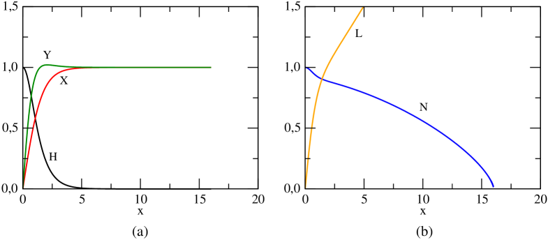
Figure 1: Non-Abelian string: In the left plot, we present the behavior for the Higgs and gauge fields as functions of $x$. In the right plot, we present the behavior of the metric functions as functions of $x$. In both plots we consider the parameters $\alpha=0.8$, $\gamma=0.61$, $\bar{\Lambda}=0.0075,$ $\beta_{2}=2.0$, $\beta_{3}=1.0$ and $q=1.0$.

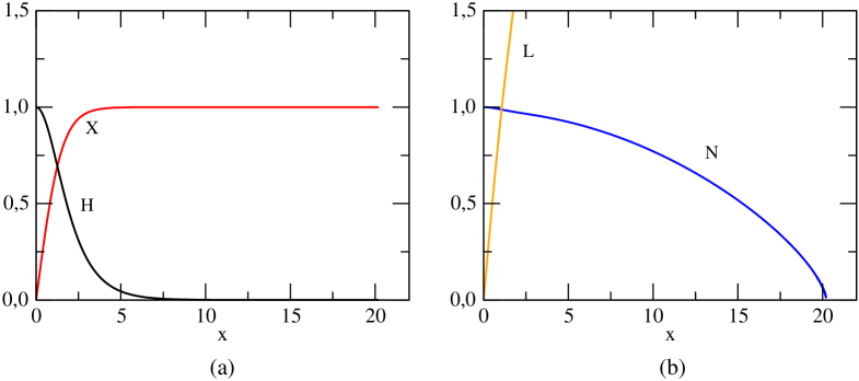
Figure 2: Abelian string: In the left plot, we present the behavior for the Higgs and gauge fields as functions of $x$. In the right plot, we present the behavior of the metric functions as functions of $x$. In both plots we consider the parameters $\alpha=0.8$, $\gamma=0.61$, $\bar{\Lambda}=0.0075$.

By comparing figure 1(b) with figure 2(b) it can be seen that both systems present cosmological horizons, $x_{0}$. Moreover, the corresponding values for the horizons for the non-Abelian system is smaller than the Abelian one. Another point that can be mentioned is that, for values of the parameters that we have chosen, the matter fields and gauge fields reach their asymptotic values in the region inside the horizons.

In the vacuum solution we have found that the cosmological horizon is reached for $x_{0}^{v}=\frac{\pi}{\sqrt{3\bar{\Lambda}}}$, which for the value of constant cosmological adopted in the plots, provides $x_{0}^{v}\approx 20.94395$. More realistic values for the cosmological horizons were obtained in both plots considering the non-trivial behaviors of the fields. Motived by this fact now we want to investigate how the cosmological horizon depends on the gravitational coupling, $\gamma$, and also on the cosmological constant itself, $\bar{\Lambda}$.

First we consider the dependence of $x_{0}$ with $\gamma$. In order to make this analysis we fixed $\alpha$, $\beta_{2}$, $\beta_{3}$, $\bar{\Lambda}$ and $q$. The value of the cosmological horizon is obtained when the metric function $N(x=x_{0})$ is zero. Our numerical results for $\alpha=0.8,\beta_{2}=2.0,\ \beta_{3}=1.0,\ \bar{\Lambda}=0.0075$ and $q=1.0$ are presented in figure 3(a). Note that the cosmological horizon decreases as the value of $\gamma$ is increased.

As to the influence of $\bar{\Lambda}$ on the cosmological horizon, we adopted a similar procedure to the case above. Nevertheless we fixed $\alpha$, $\gamma$, $\beta_{2}$, $\beta_{3}$ and $q$ and we determine the value of $x$ at which $N(x)$ vanishes. Our results are presented in figure 3(b). We clearly note that the value of cosmological constant decreases as values of $\bar{\Lambda}$ is increased. Also in this plot, we provide the behaviour for the cosmological horizon in the vacuum case.

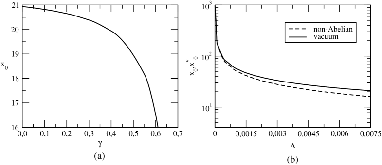
Figure 3: (a) The behavior of the cosmological horizon, $x_{0}$, as function of $\gamma$ considering the parameters $\alpha=0.8,\beta_{2}=2.0,\beta_{3}=1.0,\bar{\Lambda}=0.0075,q=1.0$. (b) The dashed line represents the behavior of the cosmological horizon, $x_{0}$, as a function of $\bar{\Lambda}$ for the non-Abelian string case, considering $\alpha=0.8,\gamma=0.61,\beta_{2}=2.0,\beta_{3}=1.0,q=1.0$. The solid line corresponds the trivial behavior of the cosmological horizon, $x_{o}^{v}$, in the vacuum case.

4.2 Anti-de Sitter Spacetime

Here, we are interested to analyze the influence of a negative cosmological constant on the behavior of the non-Abelian and Abelian cosmic string systems.

In figure 4(a) we present the behavior of the Higgs fields, $X,\ Y$, and gauge field, $H$, for the non-Abelian case as function of the dimensionless variable $x$, considering specific values attibuted to the set of parameters. In figure 4(b) we plot the behavior of the corresponding metric functions, $N$ and $L$ as function of $x$. In both plots we considered the parameters $\alpha=0.8,\ \gamma=0.6,\ \beta_{2}=2.0,\ \beta_{3}=1.0,\ \bar{\Lambda}=-0.03$ and $q=1.0$.

In figure 5(a) we present the behavior of the Higgs field, $X,$ and gauge field, $H,$ in the Abelian case for specific values attributed to set of appropriated parameters. In figure 5(b) we plot the metric functions, $N$ and $L$. In both plots we consider the parameters for Abelian case as $\alpha=0.8,\ \gamma=0.6$ and $\bar{\Lambda}=-0.03$. For both systems we can see that the function $N$ presents a strong increment for large value of $x$.

Finally we present in figure 6 the behavior of the metric fields for two different values of cosmological constant, $\bar{\Lambda}=-0.010$ and $\bar{\Lambda}=-0.007$, in the non-Abelain case with parameters $\alpha=0.8,\gamma=0.6,\beta_{2}=2.0,\beta_{3}=1.0$ and $q=1.0$. We notice that the metric field $N$ increases with the cosmological constant.

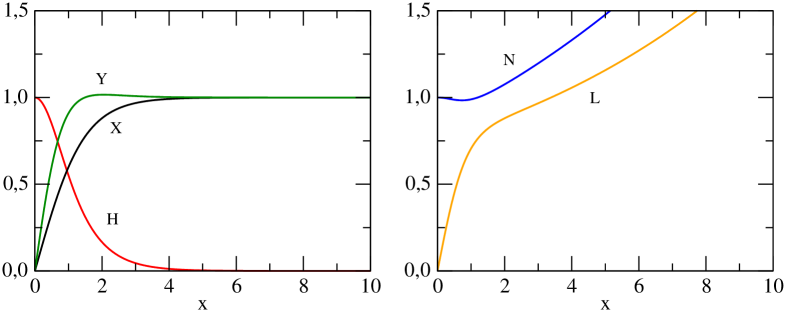
Figure 4: Non-Abelian string: In the left plot we exhibit the behavior of the Higgs and gauge fields in anti-de Sitter space. In the right plot, we present the metric functions. In both plots we have considered $\alpha=0.8,\ \gamma=0.6,\ \beta_{2}=2.0,\ \beta_{3}=1.0,\bar{\Lambda}=-0.03$ and $q=1.0$.

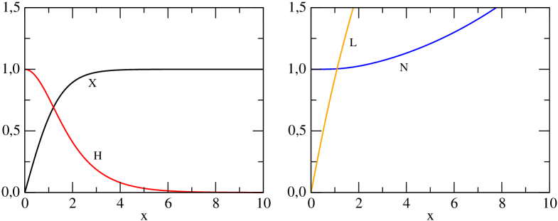
Figure 5: Abelian string: In the left plot we exhibit the behavior of the Higgs and gauge fields in anti-de Sitter space as function of $x$. In the right plot, we exhibit the behavior of the metric fields in anti-de Sitter space considering $\alpha=0.8,\gamma=0.6,\bar{\Lambda}=-0.03$.

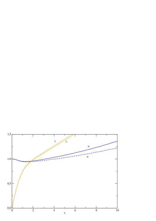
Figure 6: The metric fields as functions of $x$ for different values of cosmological constant. For solid lines we adopt $\bar{\Lambda}=-0.010$, and for dashed lines $\bar{\Lambda}=-0.007$. In both plots we consider $\alpha=0.8,\gamma=0.6,\beta_{2}=2.0,\beta_{3}=1.0$ and $q=1.0$.

4.3 Comparative analysis

In this section we would like to present plots comparing the behaviors of the metric fields, $L(x)$ and $N(x)$, as functions of $x$ for different background spacetimes: $a)$ the non-Abelian cosmic sting in Minkowski (M) and in de Sitter (dS) spacetimes, and $b)$ the non-Abelian cosmic string in Minkowski (M) and anti-de Sitter (AdS) spacetimes. In addition we have included the behaviors of these metric functions in the vacuum (vac) for dS and AdS spacetimes, given by equations (3.18), (3.19), (3.22) and (3.23). In the plots we label these curves by the subscripts $M$, $dS$, $AdS$ and $vac$, according to the space background considered. In this way we intend to point out the most relevant aspects that distinguish the behaviors of those functions. In our analysis presented in figure 7, we adopted the following values for the parameters: $\gamma=0.6,\ \alpha=0.8,\ \beta_{2}=2.0,\ \beta_{3}=1.0$ and $q=1.0$. For dS space we take $\bar{\Lambda}=0.0075$ and for AdS we take $\bar{\Lambda}=-0.03$. The behaviors of the Higgs and gauge fields are almost insensitive to the presence of a cosmological constant, for this reason we decided do not include them in the plots.

In figure 7(a) we present the behaviors of $L$ and $N$ as function of $x$ considering the non-Abelian cosmic string in Minkowski and in de Sitter spectimes. Also we present their behaviors in vacuum of de Sitter space, named vacuum solutions. We can see that the main difference is in the behaviors of the component $N$. In Minkowski space this component tends to a constant value below the unity while in dS space it goes to zero. In addition, comparing $N$ in dS with in the vacuum, we can see that the cosmological horizon for the first case is smaller that the second one. A less evident difference is in the behavior of $L$. Comparing the plot of this component in the vacuum, $L_{vac}$, in the non-Abelian string in dS, $L_{dS}$, and non-Abelian string in Mikowski, $L_{M}$, spacetimes respectively, we can notice a progressive bending. Specifically there is a small deviation between $L_{dS}$ and $L_{M}$. Another point that deserves to be mentioned is the decreasing in the slope of $L$ when one compares $L_{vac}$ with $L_{dS}$. The slope of the latter is smaller for any given point. This resembles the decreasing in the slope of $L_{M}$ when compared with the one in the vacuum in Mikowski spacetime. In fact comparing the slope of $L_{M}$ at infinity with the unity, it is possible to find a planar angle deficit by:

$$\delta/2\pi=1-L^{\prime}_{M}(\infty)=0.865\ .$$ (4.1)

In figure 7(b) we present the behaviors of $L$ and $N$ as function of $x$ considering the non-Abelian cosmic string in Minkowski and in anti-de Sitter spectimes. In addition we present their behaviors in vacuum of anti-de Sitter space. Here also we can see that the main difference in the geometry of the spacetime is given by $N$: $N_{AdS}$ increases with $x$ while $N_{M}$ presents a small decay. As to $L$ we observe that for a given value of $x$, $L_{M}$ is bigger than $L_{AdS}$; moreover, both are smaller that $L_{vac}$. So, we conclude that the non-trivial structure of the Higgs and gauge fields modify the behavior of $L$. Specifically the slope of $L_{AdS}$ is smaller that $L_{vac}$.

So, from these two plots, figures 7(a) and 7(b), two different observations deserve to be mentioned:

• The presence of a cosmological constant affects substantially the geometry of the non-Abelian cosmic string spacetime modifying mainly the components $g_{tt}=g_{zz}$ of the metric tensor.

• In the other direction we can see that the presence of matter field in dS and AdS spaces also produce relevant consequences on the behavior of the metric tensor. Specifically in dS space the value of the cosmological horizon decreases significantly.

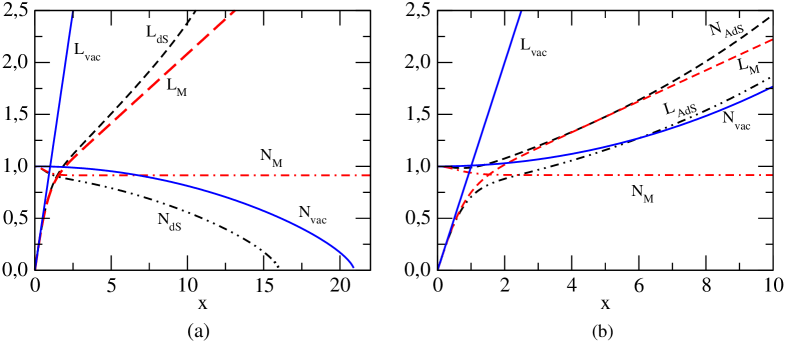
Figure 7: The metric fields $L(x)$ and $N(x)$ as functions of $x$ . (a) In figure 7(a) we compare the behavior of the metric fields $L$ and $N$ in de Sitter spacetime (dS) considering $\bar{\Lambda}=0.0075$ with the metric fields in the Minkowski (M), and with the metric fields in the respective vacuum configuration (vac). (b) In figure 7(b) we compare the behaviour of the metric fields $L$ and $N$ in anti-de Sitter spacetime (AdS) considering $\bar{\Lambda}=-0.03$ with the metric fields in the Minkowski (M) and with the metric fields in the respective vacuum configuration (vac). In both plots we consider $\gamma=0.6,\ \alpha=0.8,\beta_{2}=2.0,\beta_{3}=1.0$ and $q=1.0$.

5 Conclusion

In this paper, we have examined the influence of cosmological constant in the geometry of non-Abelian and Abelian cosmic strings spacetimes. In agreement with previous work [27], where the gravitating non-Abelian cosmic strings was studied in the absence of cosmological constant, we have shown that it is also be possible to obtain non-Abelian stable topological string considering two bosonic iso-vectors with Higgs mechanism in de Sitter and anti-de Sitter spaces.

Regarding the analysis in de Sitter space, we have shown that there appear a cosmological horizon. In fact this observation was presented in the paper by Linet for the vacuum configuration in [30], and in [21] for the Abelian string. Here we also returned to this analysis considering the non-Abelian and also Abelian strings. These investigations were presented in figures 1(b) and 2(b) for specific values of the parameters. By these graphs we have pointed out that the non-Abelian case presents a smaller cosmological horizon than corresponding Abelian one.

We also provided the behaviour of cosmological horizon, $x_{0}$, with the gravitational coupling constant, $\gamma$, and with the cosmological constant, $\bar{\Lambda}$. In figure 3(a), we can observe that the cosmological horizon decreases when one increases $\gamma$. In figure 3(b) we can see that the cosmological horizon also decreases for larger values of the cosmological constant. Moreover, we also compare this behavior with the corresponding one for the vacuum case. We see that for a given value of $\bar{\Lambda}$, the horizon associated with the vortex system is smaller than the vacuum one.

The behaviors of the Higgs and gauge fields, and metric functions in anti-de Sitter spacetime for the non-Abelian cosmic strings were displayed in figure 4. We have also shown the behaviors of Higgs and gauge fields, and metric functions for the Abelian cosmic strings in figure 5. We noticed that in both cases $N(x)$ diverges for large values of $x$; however, by our numerical results, we observe that in the non-Abelian case the slope of $N(x)$ is bigger than the corresponding Abelian one. In the figure 6, we have shown the behavior of metric fields, $N$ and $L$, as functions of $x$ for the non-Abelian system considering two different values of $\bar{\Lambda}$. By this graph and others not presented in this paper, we observe that increasing the cosmological constant the two lines, representing these functions, approach each other. This behavior is compatible with the vacuum case.

Finally we have presented in figures 7(a) and 7(b) comparative plots of the behaviors of the components $N(x)$ and $L(x)$ of the metric tensor as function of $x$, considering the non-Abelian string in Minkowski and in de Sitter backgrounds, and in Mikowski and in anti-de Sitter backgrounds, respectively. We have observed that the presence of cosmological constant strongly modifies the geometry of the spacetimes produced by the defect. The most relevant modifications are due to the component $N(x)$. For dS, $N$ goes to zero for a finite distance to the string, and for AdS this component increases. Also in these graphs we have presented the behaviors of these two functions in vacuum scenarios. By comparison of the functions in the vacuum scenarios with the full system in dS or AdS, we have observed significant deviations caused by the Higgs and gauge fields in the slopes of $L$.

References

- [1] T. W. B. Kibble, J. Phys. A 9, 1387 (1976).
- [2] T. W. B. Kibble, Some Implications of a Cosmological Phase Transition, Phys. Rep. 67, 1 (1980)
- [3] A. Vilenkin and E. S. Shellard, Cosmic strings and others topological defects. Cambridge University Press (2000).
- [4] Planck Collaboration Collaboration, P. Ade et al., Planck 2013 results XXV. Searches for cosmic strings and other topological defects, arXiv:1303.5085.
- [5] M. Hindmarsh, Signals of Inflationary Models with Cosmic Strings, Prog. Theor. Phys. Suppl. 190 (2011) 197-228, arxiv:1106.0391.
- [6] E. J. Copeland, L. Pogosian and T. Vachapati, Seeking String Theory in the Cosmos, Class. Quant. Grav. 28 (2011) 204009, arxiv:1105.0207.
- [7] H. B. Nielsen and P. Olesen, Nuclear Physics B 61, 45 (1973).
- [8] D. Garfinkle, Phys. Rev. D 31 1323 (1985).
- [9] P. Laguna-Castillo and R. A. Matzner, Phys. Rev. D 35 2933 (1987).
- [10] B. Linet, Phys. Lett. A 124, 240 (1987).
- [11] P. Laguna and D. Garfinkle, Phys. Rev. D 40, 1011 (1989).
- [12] M.E. Ortiz, Phys. Rev. D 43, 2521 (1991).
- [13] M. Christensen, A. L. Larsen and Y. Verbin, Phys. Rev. D, 60, 125012 (1999).
- [14] Y. Brihaye and M. Lubo, Phys. Rev. D, 62, 085004 (2000).
- [15] D. Kramer, H. Stephani, E. Herlt and M. MacCallum, Exact Solutions of Einstein’s Field Equations (Cambridge University Press, Cambridge, England, 1980).
- [16] B. Hartmann and J. Urrestilla, JHEP 0807 (2008) 006.
- [17] Jose J. Blanco-Pillado, Borja Reina, Kepa Sousaa and Jon Urrestilla, JCAP 1406 (2014) 001.
- [18] A. G. Riess et al., Observational Evidence from Supernovae for an Accelerating universe and Cosmological Constant, Astron. J. 116, 1009, (1998).
- [19] S. Perlmutter et al., Measurements of Omega and Lambda from 42 High-redshift Supernovae, Astrophys. J. 517, 565, (1999).
- [20] J. M. Maldacena, Adv. Theor. Math Phys. 2 231, (1998); E. Witten, Adv. Theor. Math Phys. 2 253, (1998); S. S. Gusbser, I. R. Klebanov, A. M. Polyakov, Phys. Lett. B 428, 105, (1998).
- [21] Eugênio R. Bezerra de Mello, Yves Brihaye and Betti Hartmann, Phys. Rev. D 67 124008 (2003).
- [22] A.M. Ghezelbash, R.B. Mann, Phys. Lett. B 537, 329 (2002).
- [23] Yves Brihaye and Betti Hartmann, Phys. Lett. B 669, 119 (2008).
- [24] M. Barriola and A. Vilenkin, Phys. Rev. Lett.63, 341 (1989).
- [25] Li X and Hao J, Phys. Rev. D 66 107701 (2002).
- [26] Bruno Bertrand, Yves Brihaye and Betti Hartmann, Class. Quantum Grav. 20, 4495 (2003).
- [27] Antônio de Pádua Santos and Eugênio R. Bezerra de Mello, Class. Quantum. Grav. 32 (2015) 155001.
- [28] H. J. de Vega, Phys. Rev. D 18, 2932 (1978).
- [29] Steven D. Bass, Mod. Phys. Letters A, vol. 30, No. 22, 1540033 (2015).
- [30] B. Linet, J. Math. Phys. 27, (7), 1817 (1986).
- [31] U. Ascher, J. Christiansen and R. D. Russel, Math. Comput. 33 (1979), 659; ACM Trans. Math. Softw. 7 (1981), 209.
- [32] Y. Verbin, Phys. Rev. D 59 105015 (1999).