Effect of cross-coupling on the phase behavior in a biaxial nematic: Insights from Monte Carlo studies

Abstract

Phase sequences of the biaxial nematic liquid crystal in the interior of the essential triangle are studied with Wang Landau sampling. The evidence points to the existence of an intermediate unixial phase with low biaxiality in the isotropic to biaxial nematic phase sequence.

1 Introduction

The biaxial liquid crystal phase ($N_{B}$)which was predicted in the early 70’s [1]continues to be elusive inspite of significant progress made in the theoretical[2] - [14], experimental[15] - [20] and computer simulation [21] - [27] studies regarding the existence and properties of the phase. The recent mean field theoretical (MFT) studies of a quadrupolar Hamiltonian model [5] - [9] predict a universal mean field phase diagram for biaxial nematic along the boundary of a triangular parameter space OIV( see Fig.1) wherein the condensation of the biaxial phase could occur either from the uniaxial ($N_{U}$) phase or directly from the isotropic phase ($I$). These predictions, which were partly verified by Monte Carlo simulations, were found to be unsatisfactory in the limit of vanishing biaxial-biaxial interaction in the repulsive region for the Hamiltonian, thus requiring further study.

In this context, our recent WL simulations of the phase sequences along the boundary of the triangle OIV [28, 29] suggested a qualitative modification of the MFT phase diagram as the Hamiltonian is driven to the partly repulsive regions. The efficient entropic sampling technique employed [30, 31, 32, 29] seeking otherwise inaccessible rare microstates, pointed to the existence of possible hindering free energy barriers within the system resulting from the absence of stabilising long range order of one of the molecular axes. Keeping in view the crucial role played by the degree of cross-coupling between the uniaxial and biaxial tensorial components of the neighbouring molecules in the condensation of the biaxial phase, we present in this paper, the results of a similar detailed simulation study which was carried out along a segment IW in the interior of the essential triangle, where W is the midpoint of OV (see Fig. 1).

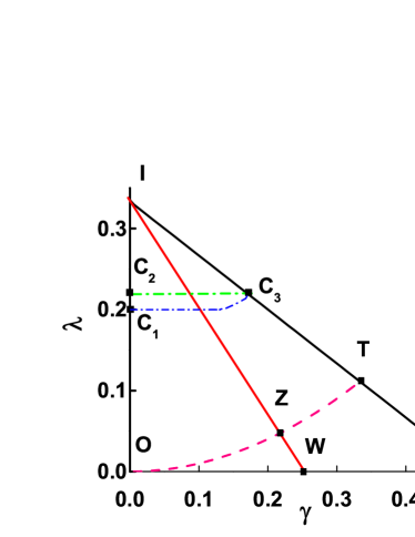
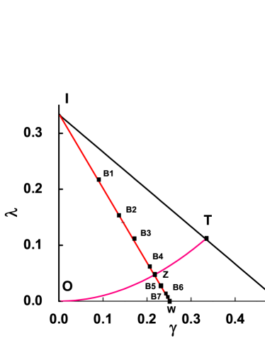
Figure 1: (a)The essential triangle, depicting the interior trajectory IZW along which detailed simulations have been carried out. (b)Location of designated values of ($\gamma,\lambda$) along IW (also see Table.(1))

We carried out a systematic simulation study using the entropic sampling technique (WL algorithm) along the segment IW in order to obtain a generic phase diagram inside the essential triangle. The mean field Hamiltonian and the simulation model are presented in section II. The sampling technique and details of simulation are discussed in section III. The observations from the simulations are reported in section IV and the conclusions are discussed in section V.

2 Hamiltonian model

The MF analysis [5] - [9], is based on the general quadrupolar orientational Hamiltonian, proposed by Straley [2] and set in terms of tensors [5]. Accordingly, the interacting biaxial molecules are represented by two pairs of symmetric, traceless tensors ($\bm{q}$, $\bm{b}$) and ($\bm{q^{{}^{\prime}}}$, $\bm{b^{{}^{\prime}}}$). Here $\bm{q}$ and $\bm{q^{{}^{\prime}}}$ are uniaxial components about the unit molecular vectors $\bm{m}$ and $\bm{m^{{}^{\prime}}}$, whereas $\bm{b}$ and $\bm{b^{{}^{\prime}}}$ (orthogonal to $\bm{q}$ and $\bm{q^{{}^{\prime}}}$, respectively), are biaxial. These irreducible components of the anisotropic parts of susceptibility tensor are represented in its eigen frame $(\bm{e},\bm{e_{\perp}},\bm{m})$ as

$$\bm{q} :=\bm{m}\otimes\bm{m}-\frac{\bm{I}}{3}$$ (1a)

$$\bm{b} :=\bm{e}\otimes\bm{e}-\bm{e}_{\perp}\otimes\bm{e}_{\perp}$$ (1b)

where $\bm{I}$ is the identity tensor. Similar representations hold for $\bm{q^{{}^{\prime}}}$ and $\bm{b^{{}^{\prime}}}$ in the eigen frame $(\bm{e^{{}^{\prime}}},\bm{e^{{}^{\prime}}_{\perp}},\bm{m^{{}^{\prime}}})$. The interaction energy is written as

$$H=-U[\xi\,\bm{q}\cdot\bm{q}^{\,\prime}+\gamma(\bm{q}\cdot\bm{b}^{\,\prime}+\bm{q}{\,\prime}\cdot\bm{b})+\lambda\,\bm{b}\cdot\bm{b}^{\,\prime}]$$ (2)

where $U$ is the scale of energy, $\xi$ = $\pm 1$, $\gamma$ and $\lambda$ are dimensionless interaction parameters, determining the relative importance of the uniaxial-biaxial coupling and biaxial-biaxial coupling interactions between the molecules, respectively.

Mean-field analysis of the Hamiltonian identifies a triangular region OIV in the $(\gamma,\lambda)$ plane - called the essential triangle - representing the domain of stability into which any physical system represented by Eqn. (2) can be mapped [7, 9] (see Fig.  1). The line $C_{1}C_{3}$ is a tricritical line whereas $C_{2}C_{3}$ is a triple line. The dispersion parabola $\lambda=\gamma^{2}$ [4] traverses through the interior of the triangle, intersecting IV at the point T, called the Landau point. Region of the triangle above the parabola corresponds to a Hamiltonian where all the terms are attractive, while the region below is noted to be partly repulsive [7]. MFT predicts a $I\rightarrow N_{U}\rightarrow N_{B}$ phase sequence in the quadrangle $OC_{2}C_{3}V$ and a direct $I\rightarrow N_{B}$ transition in the triangular region $IC_{2}C_{3}$.

For simulation purposes, the general Hamiltonian in Eqn. (2) is conveniently recast as a biaxial mesogenic lattice model, where particles of $D_{2h}$ symmetry, represented by unit vectors $\bm{u}_{a}$, $\bm{v}_{b}$ on lattice sites a and b interact through a nearest-neighbour pair potential [33]

$$U=-\epsilon\{G_{33}-2\gamma(G_{11}-G_{22})+\lambda[2(G_{11}+G_{22})-G_{33}]\}.$$ (3)

Here $f_{ab}$= ($\bm{v}_{a}$.$\bm{u}_{b}$), $G_{ab}$=$P_{2}$($f_{ab}$) with $P_{2}$ denoting the second Legendre polynomial. The constant $\epsilon$ (set to unity in simulations) is a positive quantity setting the reduced temperature $\textit{T}^{{}^{\prime}}=k_{B}\textit{T}/\epsilon$, where T is the absolute temperature of the system.

3 Details of Simulation

The Wang-Landau (WL) sampling [30] is a flat histogram technique designed to overcome energy barriers encountered, for example, near first order transitions, by facilitating a uniform random walk along the energy (E) axis through an appropriate algorithmic guidance. The sampling, originally developed for Hamiltonian models involving random walks in discrete configurational space, continues to be applied to various problems in statistical physics [34, 35], polymer and protein studies [36, 37, 38] and is being developed for more robust applications for continuous systems [39, 40, 41, 42, 43, 44, 45] and self assembly [46]. The proposed algorithm was modified [47] to suit lattice models like the Lebwohl-Lasher interaction [48], allowing for continuous variation of molecular orientations. It was subsequently augmented with the so-called frontier sampling technique [31, 32] to simulate more complex systems like the biaxial medium. The WL sampling is based on effecting a convergence of an initial distribution over energy E to the density of states (DoS) $g(E)$ of the system iteratively. Frontier sampling technique is an algorithmic guidance, provided in addition to the WL routine, by which the system is constrained to visit and sample from low entropic regions.

The simulations are performed on a cubic lattice of dimensions ($L\times L\times L,L=15and20$) with periodic boundary conditions. The biaxial liquid crystal molecule on each lattice site interacts with the nearest neighbours based on the potential in Eqn.(3). The uniaxial - biaxial coupling coefficient $\gamma$ on IW is half of the the value on the diagonal IV, for identical $\lambda$ values. We denote the arclength of the path OIW as $\lambda^{{}^{\prime}}$, given by $\lambda^{{}^{\prime}}=\lambda$ on segment OI, and

$$\lambda^{{}^{\prime}}=\dfrac{1}{3}(1+5\gamma)$$

where

$$\gamma=\dfrac{(1-3\lambda)}{4}$$

on the segment IW.

The parameters $\gamma$ and $\lambda$ were chosen such that we traverse along the path $IW$ which amounts to varying the arclength $\lambda^{{}^{\prime}}$ from  0.33 to  0.747.

Table 1: Coordinates of points B1-B7 and Z along the segment IW of the essential triangle (Fig.2)

Point	$\gamma$	$\lambda$	$\lambda^{{}^{\prime}}$
B1	0.0859	0.1719	0.4766
B2	0.1405	0.14658	0.5666
B3	0.1663	0.1116	0.6105
B4	0.2045	0.0606	0.674
Z	0.2149	0.0467	0.691
B5	0.2253	0.0328	0.709
B6	0.2440	0.0079	0.740
B7	0.2482	0.0024	0.747

The Table 1 lists the values of ($\gamma,\lambda$) and corresponding arc lengths $\lambda^{{}^{\prime}}$ at some designated points for ready reference. Fig. 1 shows the location of these points schematically inside the essential triangle. Simulations were carried out for nearly 40 points on IW using modified Wang-Landau (WL) algorithm augmented by frontier sampling. At each value, the g(E) which is the estimate of the density of states was obtained and an entropic ensemble of $10^{7}$ microstates was generated, by making an effectively uniform random walk in energy space guided by the DoS. Equilibrium ensembles at any desired (reduced) temperature ($T^{{}^{\prime}}$) are consequently extracted by a suitable reweighting procedure [31, 49] and the average values of physical properties are calculated. The representative free energy F, as a function of the energy of the system, as well as of the two dominant order parameters (uniaxial and biaxial orders) is computed from the DoS and the microcanonical energy, - both available as a function of bin number in the entropic ensemble.

The physical parameters of interest in this system, calculated at each $\lambda^{{}^{\prime}}$, are the average energy $<E>$, specific heat $<C_{v}>$, energy cumulant $V_{4}$ (= $1-<E^{4}>/(3<E^{2}>^{2})$) which is a measure of the kurtosis [50], the four order parameters of the phase calculated according to [23, 51] and their susceptibilities. These are the uniaxial order $<R^{2}_{00}>$ (along the primary director), the phase biaxiality $<R^{2}_{20}>$, and the molecular contribution to the biaxiality of the medium $<R^{2}_{22}>$, and the contribution to uniaxial order from the molecular minor axes $<R^{2}_{02}>$.

The averages are computed at a temperature resolution of 0.002 units in the temperature range [0.05, 2.05]. Statistical errors in different observables are estimated over ensembles comprising a minimum of $5\times 10^{5}$ microstates, and these are compared with several such equilibrium ensembles at the same $(\gamma,\lambda)$ value, but initiating the random walk from different arbitrary points in the configuration space. We find the relative errors in energies are 1 in $10^{5}$, while those in the estimation of the order parameters are 1 in $10^{4}$.

4 Results and Discussion

WL simulations were carried out at 40 values of $\lambda^{{}^{\prime}}$ on the segment IW, where the arc length $\lambda^{{}^{\prime}}$ ranges from 0.33 to 0.75. Temperature variation of the specific heat, and the two order parameters ($R^{2}_{00}$ and $R^{2}_{22}$) in different ranges of $\lambda^{{}^{\prime}}$, covering the segment IZ (in the attractive region of the interaction Hamiltonian), are presented in Figs. 2 - 4. The corresponding data along the segment ZW (in the repulsive region) is presented in Fig.14.

4.1 Segment IZ: Range of $\lambda^{{}^{\prime}}$ = (0.33 - 0.691)

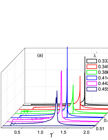
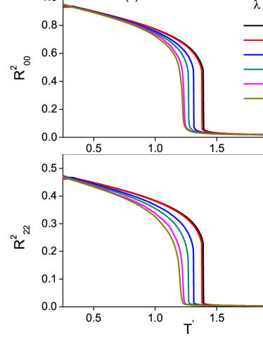
Figure 2: Comparison of (a) specific heat (b) order profiles for values of $\lambda^{{}^{\prime}}$ from 0.33 to 0.455

It is noted from Fig. 2 that for all values of $\lambda^{{}^{\prime}}$ in the range 0.33 - 0.455, a single transition peak is observed in the specific heat profile. As the biaxial system is cooled from the high temperature isotropic phase, a direct $I-N_{B}$ transition takes place and the order profiles in Fig. 2 reflect the behaviour. Fig. 3 depicts the splitting of this transition into two transitions for higher values of $\lambda^{{}^{\prime}}$ in the range 0.462 to 0.610. It is observed that lower transition temperature $T_{2}$ is progressively depressed with increase in $\lambda^{{}^{\prime}}$ value, as compared to the higher transition temperature peak at $T_{1}$.

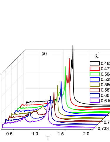
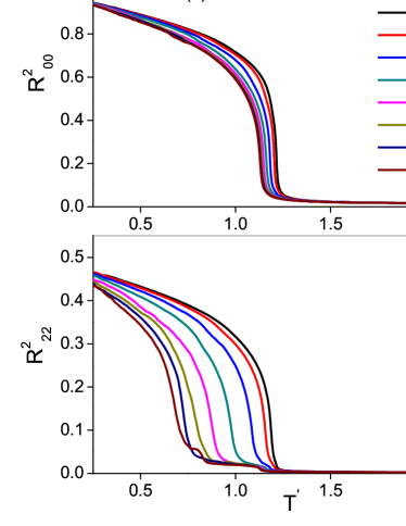
Figure 3: Comparison of (a) Specific heat (b) order parameter profiles for values of $\lambda^{{}^{\prime}}$ from 0.463 to 0.610

The variation of the order profiles in this region, shown in Fig. 3, reveals an intervening phase which is not strictly uniaxial since the system exhibits a low value of $R^{2}_{22}$ at the onset of the transition. By performing simulations at different sizes (L=10, 15, 20), the possibility that this could be a finite size effect is ruled out. (It may be noted that for these system sizes a pure uniaxial phase condenses on the $\lambda$-axis). The notable difference in the case of path IW, relative to IV, is that the degree of biaxiality (value of $R^{2}_{22}$) remains fairly independent of temperature, and the degree is the same for all subsequent values of $\lambda^{{}^{\prime}}$ beyond this threshold, until interrupted by a second low temperature transition leading to an onset of appreciable biaxial order (Fig.3).

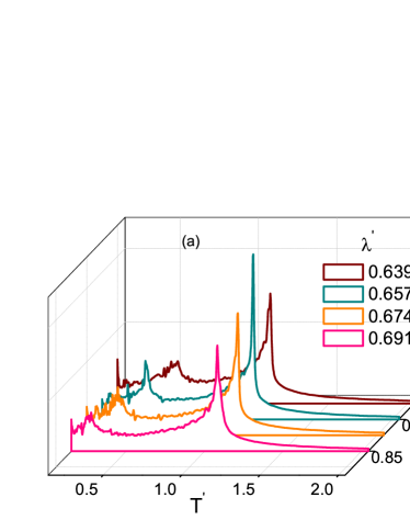
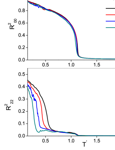
Figure 4: Comparison of (a) specific heat (b) order parameter profiles for values of $\lambda^{{}^{\prime}}$ from 0.639 to 0.691

The results of simulation for $\lambda^{{}^{\prime}}$ values in the range 0.639 - 0.691 are depicted in Fig. 4. Though these points lie very close to the parabola, they are still in the attractive region for the interaction Hamiltonian. It is observed from Fig. 4 that the second specific heat peak shifts progressively to lower temperatures as the value of $\lambda^{{}^{\prime}}$ increases. Corresponding variations in the order parameters, shown in Fig.4 confirm the shift of the second transition temperature to lower values. However it is observed that the equilibrium averages of order parameters in this region of $\lambda^{{}^{\prime}}$ are not as smooth, and show discernible fluctuations in the low temperature biaxial phase.

It is interesting to note that the intermediate phase persists to have a small degree of biaxial order ($\sim 0.05$) which (a) is not a finite size effect; (b) is fairly independent of temperatures within the liquid crystal phase; and (c) does not depend on the values of $\lambda^{{}^{\prime}}$. This phase with temperature dependence typical of uniaxial order, but having a small and constant biaxial symmetry ($\leq 0.05)$) , is designated as $N_{U^{{}^{\prime}}}$ phase in our notation. On subsequent lowering of temperature from this phase, the biaxial order increases rapidly at the second transition at $T_{2}$ and the lower temperature phase has macroscopically observable biaxial order, for all values of $\lambda^{{}^{\prime}}$.

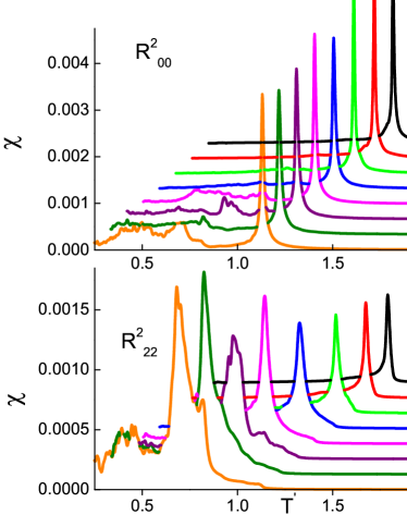
Figure 5: Susceptibilities ($\chi^{\ {}^{\prime}}$s) of the order parameters for values of $\lambda^{{}^{\prime}}$ : 0.462 - 0.610

The susceptibility profiles of the order parameter in this region are depicted in Fig. 4. It is observed that the $R^{2}_{22}$ susceptibility starts increasing in the intermediate phase before showing a peak at the low temperature transition at $T_{2}$.

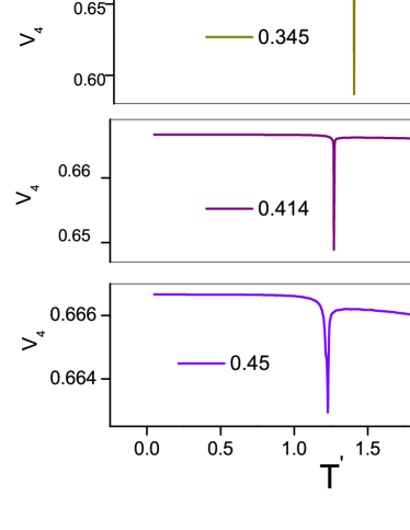
Figure 6: energy cumulant $V_{4}$ for values of $\lambda^{{}^{\prime}}$: 0.345 - 0.45

The fourth order energy cumulant ($V_{4}$) data obtained along the path OIW are shown in Figs. 6 - 8. It is observed that the $I-N_{B}$ transition remains strongly first order for values of $\lambda^{{}^{\prime}}$ from 0.345 to 0.45. In the range of $\lambda^{{}^{\prime}}$ from 0.463 to 0.691 ( i.e upto the point Z in Fig.1), the high temperature transition at $T_{1}$ from the isotropic phase (I) to the ordered $N_{U^{{}^{\prime}}}$ phase shows a first order nature. Subsequently, the low temperature $N_{U^{{}^{\prime}}}-N_{B}$ transition seems to change gradually from first order to continuous nature, as seen from $V_{4}$ profiles in Figs.6 and 8.

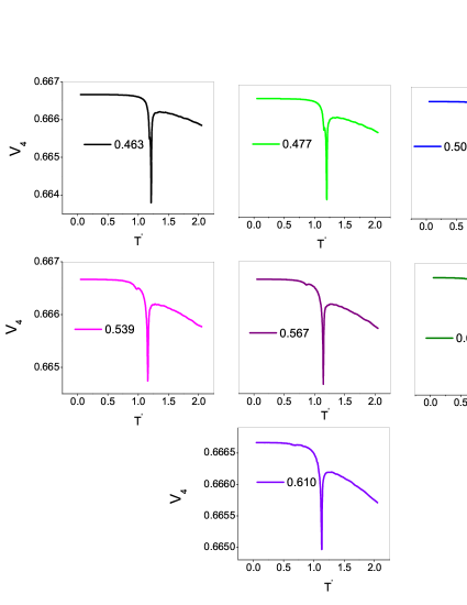
Figure 7: Energy cumulant $V_{4}$ for values of $\lambda^{{}^{\prime}}$ :0.463 - 0.610

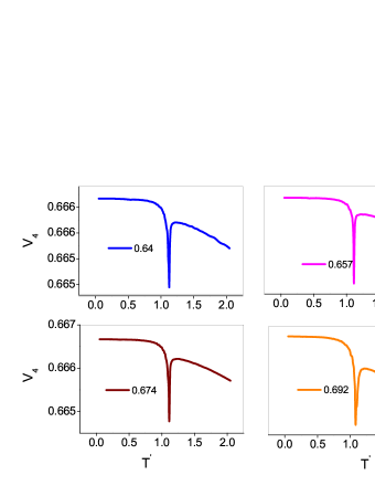
Figure 8: energy cumulant $V_{4}$ for values of $\lambda^{{}^{\prime}}$ : 0.64 - 0.691

An analysis of the above simulation data leads to the proposal of a phase diagram along the path IW, shown in Fig.9. We could report the $L=20$ data only upto the value $\lambda^{{}^{\prime}}=0.709$, as beyond this value (which falls into the partly repulsive region under the parabola) the computational times for the convergence of DoS are impractical.

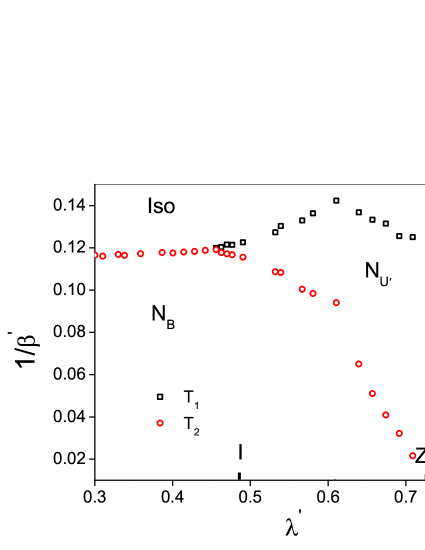
Figure 9: Phase diagram inside the essential triangle along path IW

We observe from the temperature variation of order parameters that the growth of biaxial order appears to be progressively inhibited as $\lambda^{{}^{\prime}}$ value increases within the attractive region, and enters the party repulsive region on crossing the parabola at the point Z. The free energy profiles, plotted as a function of energy and order parameters (computed from the DOS data), reflect the rationale for the impediments for the growth of the biaxial order as the base of the triangle OIW is reached.

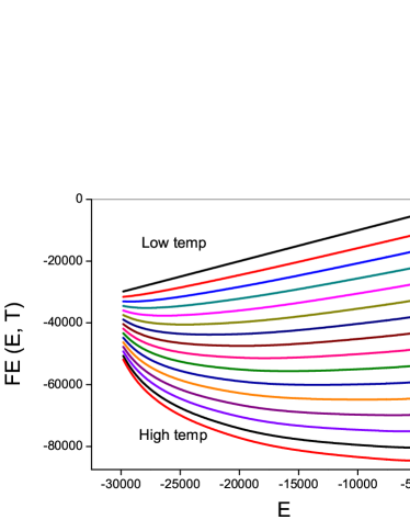
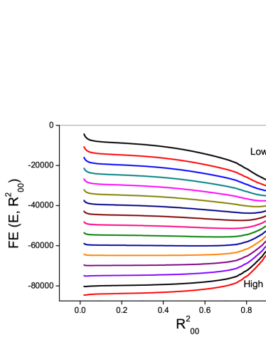
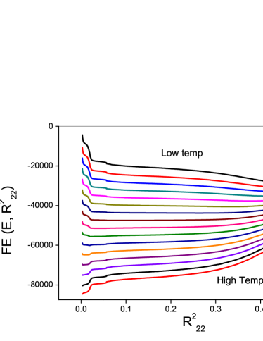
Figure 10: Representative free energy plotted as a function of (a) energy (b)$R^{2}_{00}$ (c) $R^{2}_{22}$ at the point B3 ($\lambda^{{}^{\prime}}$ = 0.610 )

The free energy curves obtained for $\lambda^{{}^{\prime}}$= 0.610 ($B_{3}$in the attractive region) are shown in Fig. 10. These curves depict the smooth variation of free energy as a function of energy and uniaxial order parameter. However, its variation with respect to $R^{2}_{22}$ shows a small sharp well, (the edge being located at $R^{2}_{22}\simeq 0.02$), and the family of curves in Fig.10, as a function of temperature, shows that it required significant variation of temperature before the system could shift its free energy minimum away from this restricted region. It appears that during this temperature range, the system accesses microstates with rather small but nonzero degree of biaxiality, constrained however by free energy barriers to attain higher degree of biaxiality for considerable range of temperature. This circumstance seems to be manifesting as a corresponding curious variation of $R^{2}_{22}$ at $\lambda^{{}^{\prime}}$= 0.610, as in Fig.LABEL:fig:. We find that the development of such free energy barriers (with respect to $R^{2}_{22}$ at low values) and the requirement of the system to cool sufficiently to overcome them before accessing higher macroscopically observable values, is generic. All the data collected in this region supports and corroborates the simulated order parameter profiles reported in the previous figures. It is very interesting that such barriers are exhibited only along the path of biaxial order, but not along energy or uniaxial order. This implies a complex free energy surface in the 2-d space of order parameter, offering initial barriers to a significant development of biaxial order, until the system is sufficiently cooled. Figs. 11 - 13 demonstrate this view point.

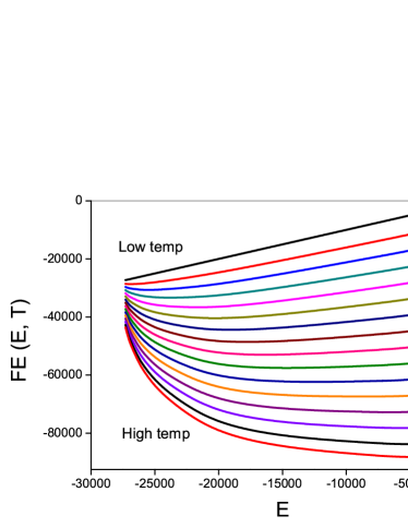
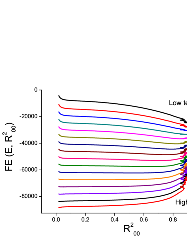
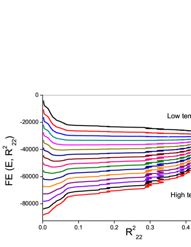
Figure 11: Representative free energy plotted as a function of (a) energy (b)$R^{2}_{00}$ (c) $R^{2}_{22}$ at the point B4 ($\lambda^{{}^{\prime}}$ = 0.674)

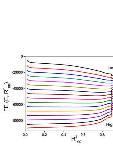
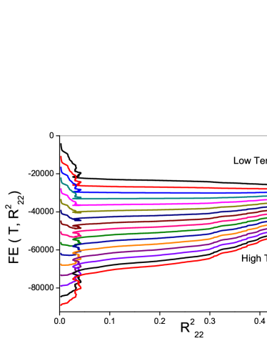
Figure 12: Representative free energy plotted as a function of (a) energy (b) $R^{2}_{00}$ (c) $R^{2}_{22}$ at the point Z ($\lambda^{{}^{\prime}}$ = 0.691)

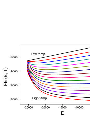
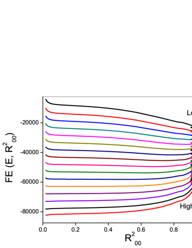
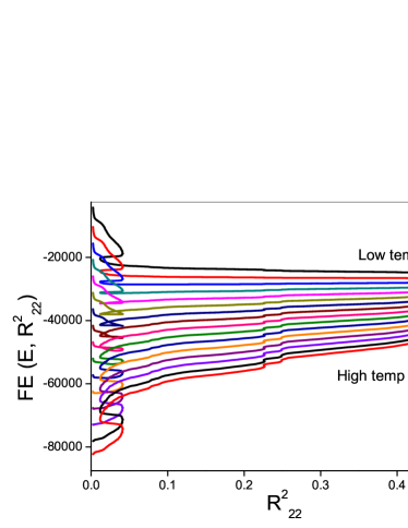
Figure 13: Representative free energy plotted as a function of (a) energy (b) $R^{2}_{00}$ (c) $R^{2}_{22}$ at the point B5 ($\lambda^{{}^{\prime}}$ = 0.709)

4.2 Segment ZW: Range of $\lambda^{{}^{\prime}}$ = (0.691 - 0.747)

We now present data obtained beyond the point Z (Fig.LABEL:fig:e2). In this region, the biaxial-biaxial tensorial coupling term $\lambda\rightarrow 0$ asymptotically, leading to a special case of the interaction Hamiltonian. The case for $\lambda$ = 0 was studied earlier through simulations [21]. It was found that in the absence of the biaxial-biaxial interaction term, only a uniaxial phase could be obtained on condensation from the isotropic phase. We present here the simulation results in the case of $\lambda\rightarrow 0$. The mean field analysis predicts that the Hamiltonian is partly repulsive in this region and excluded volume effects play a major role [8].

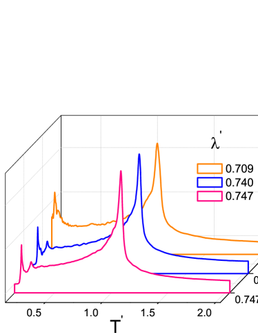
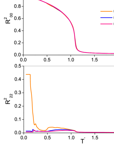
Figure 14: Comparison of (a) specific heat (b) order parameter profiles for values of $\lambda^{{}^{\prime}}$ in the range 0.709 - 0.747 (L=15)

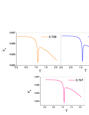
Figure 15: Energy cumulant $V_{4}$ for values of $\lambda^{{}^{\prime}}$ in the range 0.709 - 0.747 (L=15)

Due to the constraints imposed by computational time, we could obtain data in this range of $\lambda^{{}^{\prime}}$ only for a smaller system, with L=15. (instead of L=20, as in the earlier case). The specific heat and order parameter profiles are depicted in Figs. 14 and 14. The energy cumulants $V_{4}$ are shown in Fig. 15. It may be observed that the specific heat profiles show evidences of two transitions. The order parameter profiles depict the onset and growth of uniaxial order at $T_{1}$ for all values of $\lambda^{{}^{\prime}}$. The biaxial order parameter increases at $T_{2}$ (in the biaxial phase) for $\lambda^{{}^{\prime}}$ = 0.709, but remains close to zero for $\lambda^{{}^{\prime}}$ = 0.740 and 0.747. This behaviour is as expected from mean field considerations at such values of $\lambda^{{}^{\prime}}$, very close to the base OW.

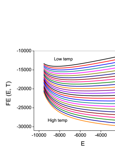
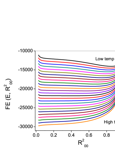
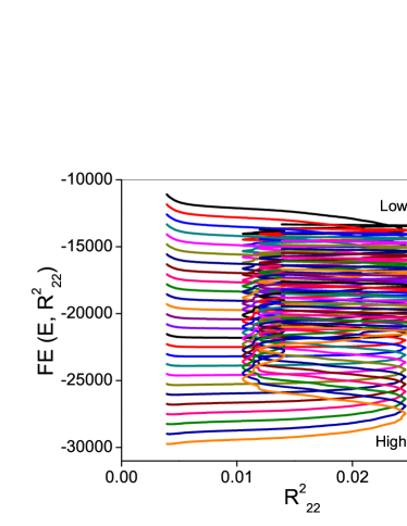
Figure 16: Representative free energy plotted as a function of (a) energy (b)$R^{2}_{00}$ (c) $R^{2}_{22}$ at point B6 ($\lambda^{{}^{\prime}}$ = 0.740)

The free energy plots for $\lambda^{\textbullet}$ = 0.740 are shown in Figs. 16 - 16. The free energy variation with respect to $R^{2}_{22}$ for $\lambda^{{}^{\prime}}$ = 0.740 again confirms the presence of barriers for the growth of biaxial order at points close to the base OW. The biaxial state is obviously not stable at such parameter points of the Hamiltonian.

5 Conclusions

In this paper, the interior of essential triangle is explored with entropic sampling method along a trajectory IW, a line drawn from apex I of the triangle to the mid point W of the base OV (Fig. 1). We refer to the arc length OIW as $\lambda^{{}^{\prime}}$, for purposes of discussion. As per MF treatment this line cuts both the trajectories of $C_{2}C_{3}$ and $C_{1}C_{3}$. Thus the phase sequences along this line IW should be qualitatively similar to that on the $\lambda$-axis. In particular the direct transition from isotropic to biaxial phase is expected to be interrupted by a uniaxial nematic phase beyond a value as $\gamma$ increases, and the temperature range of the uniaxial phase should progressively increase, suppressing the second transition temperature, till the line cuts the parabola, at Z (Fig.1). Results from mean field treatment in the partly repulsive region on this line IW are not available for direct comparison, even though it is established that biaxial phase would not be stable at the point W [9, 52]. The phase sequences in the present work qualitatively follow this scenario, but with a curious deviation. The intervening ”uniaxial ” phase $N_{U}$ is not strictly devoid of biaxial symmetry. Indeed all along the line, beyond $K^{{}^{\prime}}$ (Fig.LABEL:fig:e1), and upto point Z, the onset of the uniaxial order is invariably accompanied by a small, but unmistakable, development of biaxial symmetry. We thus refer to this phase as $N_{U^{{}^{\prime}}}$, to make this subtle distinction. This small degree of biaxiality of the $N_{U^{{}^{\prime}}}$ phase is temperature independent within that phase, and is also fairly independent of its location in the trajectory beyond $K^{{}^{\prime}}$. An examination of the free energy profiles, drawn as a function of both the major order parameters, show interesting features: while the free energy curves show smooth variation of the minima with respect to $R^{2}_{00}$ as the temperature is varied, the case of $R^{2}_{22}$ is qualitatively different. These profiles exhibit free energy barriers at low values of $R^{2}_{22}$, which could be overcome (thereby pushing the system to access regions of higher and discernible order), only after these initial barriers could be overcome on considerable cooling. Thus these results show a complex free energy surface that develops with decrease of temperature on a typical trajectory inside the triangle. It appears that development of a $N_{U^{{}^{\prime}}}$ phase with a small biaxial order ($\leq 0.05)$ is expected, and the degree of this symmetry is restricted by the free energy barriers till the system is permitted to access these regions of biaxial order. Given that such barriers are strongly dependent on the size of the system, it is a plausible conjecture to suggest that in real systems these barriers are not readily overcome (or equivalently, requires significant cooling of the medium), and hence their biaxial order appears to be restricted inherently. Under such circumstances requiring wider temperature ranges to overcome barriers, real systems may have other competing interactions (like translational degrees, influencing the phase sequence qualitatively differently , e.g layer formation). Deviations of real systems from MF predictions [53] could perhaps be understood in these terms.

References

- [1] M. J. Freiser, Phys. Rev. Lett. 24, 1041 (1970).
- [2] J. P. Straley, Phys. Rev. A 10, 1881 (1974).
- [3] D. K. Remler, and A. D. J. Haymet, J. Phys. Chem., 90, 5426 (1986).
- [4] G. R. Luckhurst, C. Zannoni, P. L. Nordio, and U. Segre, Mol. Phys. 30, 1345 (1975).
- [5] A. M. Sonnet, E. G. Virga, and G. E. Durand, Phys. Rev. E 67, 061701 ( 2003).
- [6] G. De Matteis, and E. G. Virga, Phys. Rev. E 71, 061703 (2005).
- [7] F. Bisi, E. G. Virga, E. C. Gartland Jr., G. De Matteis, A. M. Sonnet, and G. E. Durand, Phys. Rev. E 73, 051709 (2006).
- [8] F. Bisi, S. Romano, and E. G. Virga, Phys. Rev. E 75, 041705 ( 2007)
- [9] G. De Matteis, F. Bisi, and E. G. Virga, Continuum. Mech. Thermodynamics. 19, 1 (2007).
- [10] R. Alben, Phys. Rev. Lett. 30, 778 (1973).
- [11] N. Bocara, R. Mejdani, and L. De Seze, J. Phys. (Paris) 38, 149 (1976).
- [12] E. F. Gramsbergen, L. Longa, and W. H. de Jeu, Phys. Rep. 135, 195 (1986).
- [13] D. Allender and L. Longa, Phy. Rev. E 78, 011704 (2008).
- [14] P. K. Mukherjee and Kallol Sen, J. Chem. Phys. 130, 141101 (2009).
- [15] L. J. Yu and A. Saupe, Phys. Rev. Lett. 45, 1000 (1980).
- [16] B. R. Acharya, A. Primak and S. Kumar, Phys. Rev. Lett. 92, 145506 (2004).
- [17] L. A. Madsen, T. J. Dingemans, M. Nakata, and E. T. Samulski, Phys. Rev. Lett. 92, 145505 (2004).
- [18] K. Merkel, A. Kocot, J. K. Vij, R. Korlacki, G. H. Mehl, and T. Meyer, Phys. Rev. Lett. 93, 237801 (2004).
- [19] J. L. Figueirinhas, C. Cruz, D. Filip, G. Feio, A. C. Ribeiro, Y. Frere, T. Meyer, and G. H. Mehl, Phys. Rev. Lett. 94, 107802 (2005).
- [20] K. Severing and K. Saalwachter, Phys. Rev. Lett. 92, 125501 (2004).
- [21] G. R. Luckhurst and S. Romano, Mol. Phys. 40, 129 (1980).
- [22] M. P. Allen. Liq. Cryst. 8, 499 (1990).
- [23] F. Biscarini, C. Chiccoli, P. Pasini, F. Semeria, and C. Zannoni, Phys. Rev. Lett. 75, 1803 (1995).
- [24] C. Chiccoli, P. Pasini, F. Semeria, and C. Zannoni, Int. J. Mod. Phys. C 10, 469 (1999).
- [25] R. Berardi and C. Zannoni, Mol. Cryst. Liq. Cryst. 396, 177 (2003).
- [26] R. Berardi, L. Muccioli, S. Orlandi, M. Ricci and C. Zannoni, J. Phys.: Condens. Matter 20, 463101 (2008).
- [27] G. De Matteis, S. Romano, and E. G. Virga, Phys. Rev. E 72, 041706 (2005).
- [28] B. Kamala Latha, Regina Jose, K. P. N. Murthy and V. S. S. Sastry, Phys. Rev. E 89, 050501(R) (2014).
- [29] B. Kamala Latha, Regina Jose, K. P. N. Murthy and V. S. S. Sastry, Phys. Rev. E 92, 012505 (2015).
- [30] F. Wang and D. P. Landau, Phys. Rev. Lett. 86, 2050 (2001); F. Wang and D. P. Landau, Phys. Rev. E 64, 056101 (2001).
- [31] C. Zhou, T. C. Schulthess, S. Torbrugge, and D. P. Landau, Phys. Rev. Lett. 96, 120201 (2006).
- [32] D. Jayasri, Ph. D Thesis, Non-Boltzmann Monte Carlo study of Confined Liquid Crystals and Liquid Crystal Elastomers, University of Hyderabad, India (2009).
- [33] S. Romano, Physica A 337, 505 (2004).
- [34] D. P. Landau and K. Binder, A Guide to Monte Carlo Simulations in Statistical Physics, Cambridge University Press, 2nd edition(2005).
- [35] K. P. N. Murthy, Monte Carlo Methods in Statistical Physics Universities Press, India(2004).
- [36] N. Rathore, T. A. Knotts and J. J. de Pablo, Biophysics. J. 85, 3963 (2003).
- [37] D. T. Seaton, T. Wust and D. P. Landau, Phys. Rev. E 81, 011802 (2010).
- [38] Priya Singh, Subir. K. Sarkar and Pradipta Bandyopadhyay, Chem. Phys. Lett. 514, 357 (2011).
- [39] P. Poulain, F. Calvo, R. Antoine, M. Broyer and P. Dugourd, Phys. Rev. E 73, 056704 (2006).
- [40] S. Sinha and S. K. Roy, Phys. Lett. A 373, 308 (2009).
- [41] Raj Shekhar, Jonathan K. Whitmer, Rohit Malshe, J. A. Moreno-Razo, Tyler F. Roberts and Juan J. de Pablo, J. Chem. Phys. 136, 234503(2012).
- [42] Yang Wei Koh and Hwee Kuan Lee, Phys. Rev. E 88, 053302 (2013).
- [43] T. Vogel, Y. W. Li, T. Wust and D. P. Landau, Phys. Rev. Lett. 110, 210603 (2013).
- [44] Katie A. Maerzke, Lili Gai, Peter T. Cummings and Clare McCabe, J. Phys. Conference Series 487, 012002 (2014).
- [45] Y. L. Xie, P. Chu, Y. L. Wang, J. P. Chen, Z. B. Yan, J. -M. Liu, Phys. Rev. E 89, 013311 (2014).
- [46] Lili Gai, Thomas Vogel, Katie A. Maerzke, Christopher R. lacovella, David P. Landau, Peter T. Cummings and Clare McCabe, J. Chem. Phys. 139, 054505 (2013).
- [47] D. Jayasri, V. S. S. Sastry, and K. P. N. Murthy, Phys. Rev. E 72, 036702 (2005).
- [48] P. A. Lebwohl and G. Lasher, Phys. Rev. A 6, 426 ( 1972).
- [49] R. H. Swendsen and J. S. Wang, Phys. Rev. Lett. 58, 86 (1987).
- [50] K. Binder, Z. Physik. B 43, 119 (1981); K. Binder, Phys. Rev. Lett. 47, 693 (1981).
- [51] Robert J Low, Eur. J. Phys. 23, 111 ( 2002).
- [52] G. De Matteis and S. Romano, Phys. Rev. E 78, 021702 (2008).
- [53] F. Bisi, G. R. Luckhurst, E. G. Virga, Phy. Rev. E 78, 021710 (2008).