Rigid Body Motion Estimation based on the Lagrange-d’Alembert Principle

Abstract

Stable estimation of rigid body pose and velocities from noisy measurements, without any knowledge of the dynamics model, is treated using the Lagrange-d’Alembert principle from variational mechanics. With body-fixed optical and inertial sensor measurements, a Lagrangian is obtained as the difference between a kinetic energy-like term that is quadratic in velocity estimation error and the sum of two artificial potential functions; one obtained from a generalization of Wahba’s function for attitude estimation and another which is quadratic in the position estimate error. An additional dissipation term that is linear in the velocity estimation error is introduced, and the Lagrange-d’Alembert principle is applied to the Lagrangian with this dissipation. This estimation scheme is discretized using discrete variational mechanics. The presented pose estimator requires optical measurements of at least three inertially fixed landmarks or beacons in order to estimate instantaneous pose. The discrete estimation scheme can also estimate velocities from such optical measurements. In the presence of bounded measurement noise in the vector measurements, numerical simulations show that the estimated states converge to a bounded neighborhood of the actual states.

1 INTRODUCTION

Estimation of rigid body translational and rotational motion is indispensable for operations of spacecraft, unmanned aerial and underwater vehicles. Autonomous state estimation of a rigid body based on inertial vector measurement and visual feedback from stationary landmarks, in the absence of a dynamics model for the rigid body, is analyzed here. This estimation scheme can enhance the autonomy and reliability of unmanned vehicles in uncertain GPS-denied environments. Salient features of this estimation scheme are: (1) use of onboard optical and inertial sensors, with or without rate gyros, for autonomous navigation; (2) robustness to uncertainties and lack of knowledge of dynamics; (3) low computational complexity for easy implementation with onboard processors; (4) proven stability with large domain of attraction for state estimation errors; and (5) versatile enough to estimate motion with respect to stationary as well as moving objects. Robust state estimation of rigid bodies in the absence of complete knowledge of their dynamics, is required for their safe, reliable, and autonomous operations in poorly known conditions. In practice, the dynamics of a vehicle may not be perfectly known, especially when the vehicle is under the action of poorly known forces and moments. The scheme proposed here has a single, stable algorithm for the coupled translational and rotational motion of rigid bodies using onboard optical (which may include infra-red) and inertial sensors. This avoids the need for measurements from external sources, like GPS, which may not be available in indoor, underwater or cluttered environments [11].

Attitude estimators using unit quaternions for attitude representation may be unstable in the sense of Lyapunov, unless they identify antipodal quaternions with a single attitude. This is also the case for attitude control schemes based on continuous feedback of unit quaternions, as shown in [1]. One adverse consequence of these unstable estimation and control schemes is that they end up taking longer to converge compared with stable schemes under similar initial conditions and initial transient behavior. Continuous-time attitude observers and filtering schemes on $\mathrm{SO(3)}$ and $\mathrm{SE(3)}$ have been reported in, e.g., [2, 10, 12, 16, 19]. These estimators do not suffer from kinematic singularities like estimators using coordinate descriptions of attitude, and they do not suffer from unwinding as they do not use unit quaternions. The maximum-likelihood (minimum energy) filtering method of Mortensen [15] was recently applied to attitude estimation, resulting in a nonlinear attitude estimation scheme that seeks to minimize the stored “energy” in measurement errors [21]. This scheme is obtained by applying Hamilton-Jacobi-Bellman (HJB) theory to the state space of attitude motion. Since the HJB equation can only be approximately solved with increasingly unwieldy expressions for higher order approximations, the resulting filter is only “near optimal” up to second order. Unlike filtering schemes that are based on approximate or “near optimal” solutions of the HJB equation and do not have provable stability, the estimation scheme obtained here is shown to be almost globally asymptotically stable. Moreover, unlike filters based on Kalman filtering, the estimator proposed here does not presume any knowledge of the statistics of the initial state estimate or the sensor noise. Indeed, for vector measurements using optical sensors with limited field-of-view, the probability distribution of measurement noise needs to have compact support, unlike standard Gaussian noise processes that are commonly used to describe such noisy measurements.

The variational attitude estimator recently appeared in [7], where it was shown to be almost globally asymptotically stable. Some of the advantages of this scheme over some commonly used competing schemes are reported in [6]. This paper is the variational estimation framework to coupled rotational (attitude) and translational motion, as exhibited by maneuvering vehicles like UAVs. In such applications, designing separate state estimators for the translational and rotational motions may not be effective and may lead to poor navigation. Moreover, like other vision-inertial navigation schemes [18], the estimation scheme proposed here does not rely on GPS. However, unlike many other vision-inertial estimation schemes, the estimation scheme proposed here can be implemented without any direct velocity measurements. Since rate gyros are usually corrupted by high noise content and bias [3, 4, 5], such a velocity measurement-free scheme can result in fault tolerance in the case of faults with rate gyros. Additionally, this estimation scheme can be extended to relative pose estimation between vehicles from optical measurements, without direct communications or measurements of relative velocities.

2 NAVIGATION USING OPTICAL AND INERTIAL SENSORS

Consider a vehicle in spatial (rotational and translational) motion.

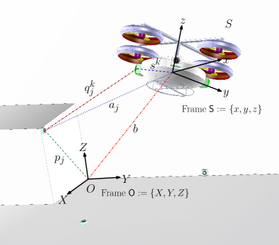
Figure 1: Inertial landmarks on $O$ as observed from vehicle $S$ with optical measurements.

Onboard estimation of the pose of the vehicle involves assigning a coordinate frame fixed to the vehicle body, and another coordinate frame fixed in the environment which takes the role of the inertial frame. Let $O$ denote the observed environment and $S$ denote the vehicle. Let $\mathsf{S}$ denote a coordinate frame fixed to $S$ and $\mathsf{O}$ be a coordinate frame fixed to $O$, as shown in Fig. 1. Let $R\in\mathrm{SO(3)}$ denote the rotation matrix from frame $\mathsf{S}$ to frame $\mathsf{O}$ and $b$ denote the position of origin of $\mathsf{S}$ expressed in frame $\mathsf{O}$. The pose (transformation) from body fixed frame $\mathsf{S}$ to inertial frame $\mathsf{O}$ is then given by

$$\mathsf{g}=\begin{bmatrix}R\;\;\;&b\\ 0\;\;\;&1\end{bmatrix}\in\mathrm{SE(3)}.$$ (1)

Consider vectors known in inertial frame $\mathsf{O}$ measured by inertial sensors in the vehicle-fixed frame $\mathsf{S}$; let $\beta$ be the number of such vectors. In addition, consider position vectors of a few stationary points in the inertial frame $\mathsf{O}$ measured by optical (vision or lidar) sensors in the vehicle-fixed frame $\mathsf{S}$. Velocities of the vehicle may be directly measured or can be estimated by linear filtering of the optical position vector measurements [8]. Assume that these optical measurements are available for $\mathpzc j$ points at time $t$, whose positions are known in frame $\mathsf{O}$ as $p_{j}$, $j\in\mathcal{I}(t)$, where $\mathcal{I}(t)$ denotes the index set of beacons observed at time $t$. Note that the observed stationary beacons or landmarks may vary over time due to the vehicle’s motion. These points generate ${\mathpzc j\choose 2}$ unique relative position vectors, which are the vectors connecting any two of these landmarks. When two or more position vectors are optically measured, the number of vector measurements that can be used to estimate attitude is ${\mathpzc j\choose 2}+\beta$. This number needs to be at least two (i.e., ${\mathpzc j\choose 2}+\beta\geq 2$) at an instant, for the attitude to be uniquely determined at that instant. In other words, if at least two inertial vectors are measured at all instants (i.e., $\beta\geq 2$), then beacon position measurements are not required for estimating attitude. However, at least one beacon or feature point position measurement is still required to estimate the position of the vehicle.

2-A Pose Measurement Model

Denote the position of an optical sensor and the unit vector from that sensor to an observed beacon in frame $\mathsf{S}$ as $s^{k}\in\mathbb{R}^{3}$ and $u^{k}\in\mathbb{S}^{2}$, $k=1,\ldots,\mathpzc k$, respectively. Denote the relative position of the $j^{th}$ stationary beacon observed by the $k^{th}$ sensor expressed in frame $\mathsf{S}$ as $q^{k}_{j}$. Thus, in the absence of measurement noise

$$p_{j}=R(q^{k}_{j}+s^{k})+b=Ra_{j}+b,\;j\in\mathcal{I}(t),$$ (2)

where $a_{j}=q^{k}_{j}+s^{k}$, are positions of these points expressed in $\mathsf{S}$. In practice, the $a_{j}$ are obtained from range measurements that have additive noise, which we denote as $a_{j}^{m}$. In the case of lidar range measurements, these are given by

$$a_{j}^{m}=(q^{k}_{j})^{m}+s^{k}=(\varrho_{j}^{k})^{m}u^{k}+s^{k},\;j\in\mathcal{I}(t),$$ (3)

where $(\varrho_{j}^{k})^{m}$ is the measured range to the point by the $k^{th}$ sensor. The mean of the vectors $p_{j}$ and $a_{j}^{m}$ are denoted as $\bar{p}$ and $\bar{a}^{m}$ respectively, and satisfy

$$\bar{a}^{m}=R^{\mbox{\small T}}(\bar{p}-b)+\bar{\varsigma},$$ (4)

where $\bar{p}=\frac{1}{\mathpzc j}\sum\limits j_{j=1}p_{j}$, $\bar{a}^{m}=\frac{1}{\mathpzc j}\sum\limits j_{j=1}a_{j}^{m}$ and $\bar{\varsigma}$ is the additive measurement noise obtained by averaging the measurement noise vectors for each of the $a_{j}$. Consider the ${\mathpzc j\choose 2}$ relative position vectors from optical measurements, denoted as $d_{j}=p_{\lambda}-p_{\ell}$ in frame $\mathsf{O}$ and the corresponding vectors in frame $\mathsf{S}$ as $l_{j}=a_{\lambda}-a_{\ell}$, for $\lambda,\ell\in\mathcal{I}(t)$, $\lambda\neq\ell$. The $\beta$ measured inertial vectors are included in the set of $d_{j}$, and their corresponding measured values expressed in frame $\mathsf{S}$ are included in the set of $l_{j}$. If the total number of measured (optical and inertial) vectors, ${\mathpzc j\choose 2}+\beta=2$, then $l_{3}=l_{1}\times l_{2}$ is considered a third measured direction in frame $\mathsf{S}$ with corresponding vector $d_{3}=d_{1}\times d_{2}$ in frame $\mathsf{O}$. Therefore,

$$d_{j}=Rl_{j}\Rightarrow D=RL,$$ (5)

where $D=[d_{1}\;\,\cdots\;\,d_{n}]$, $L=[l_{1}\;\,\cdots\;\,l_{n}]\in\mathbb{R}^{3\times n}$ with $n=3$ if ${\mathpzc j\choose 2}+\beta=2$ and $n={\mathpzc j\choose 2}+\beta$ if ${\mathpzc j\choose 2}+\beta>2$. Note that the matrix $D$ consists of vectors known in frame $\mathsf{O}$. Denote the measured value of matrix $L$ in the presence of measurement noise as $L^{m}$. Then,

$$L^{m}=R^{\mbox{\small T}}D+\mathscr{L},$$ (6)

where $\mathscr{L}\in\mathbb{R}^{3\times n}$ consists of the additive noise in the vector measurements made in the body frame $\mathsf{S}$.

2-B Velocities Measurement Model

Denote the angular and translational velocity of the rigid body expressed in frame $\mathsf{S}$ by $\Omega$ and $\nu$, respectively. Thus, one can write the kinematics of the rigid body as

$$\dot{\Omega}=R\Omega^{\times},\dot{b}=R\nu\Rightarrow\dot{\mathsf{g}}=\mathsf{g}\xi^{\vee},$$ (7)

where $\xi=\begin{bmatrix}\Omega\\ \nu\end{bmatrix}\in\mathbb{R}^{6}$ and $\xi^{\vee}=\begin{bmatrix}\Omega^{\times}&\;\nu\\ 0\;\;&0\end{bmatrix}$ and $(\cdot)^{\times}:\mathbb{R}^{3}\to\mathfrak{so}(3)\subset\mathbb{R}^{3\times 3}$ is the skew-symmetric cross-product operator that gives the vector space isomorphism between $\mathbb{R}^{3}$ and $\mathfrak{so}(3)$. For the general development of the motion estimation scheme, it is assumed that the velocities are directly measured. The estimator is then extended to cover the cases where: (i) only angular velocity is directly measured; and (ii) none of the velocities are directly measured.

3 DYNAMIC ESTIMATION OF MOTION FROM PROXIMITY MEASUREMENTS

In order to obtain state estimation schemes from measurements as outlined in Section 2 in continuous time, the Lagrange-d’Alembert principle is applied to an action functional of a Lagrangian of the state estimate errors, with a dissipation term linear in the velocities estimate error. This section presents the estimation scheme obtained using this approach. Denote the estimated pose and its kinematics as

$$\hat{\mathsf{g}}=\begin{bmatrix}\hat{R}&\;\;\;\hat{b}\\ 0&\;\;\;1\end{bmatrix}\in\mathrm{SE(3)},\;\;\dot{\hat{\mathsf{g}}}=\hat{\mathsf{g}}\hat{\xi}^{\vee},$$ (8)

where $\hat{\xi}$ is rigid body velocities estimate, with $\hat{\mathsf{g}}_{0}$ as the initial pose estimate and the pose estimation error as

$$\mathsf{h}=\mathsf{g}\hat{\mathsf{g}}^{-1}=\begin{bmatrix}Q&\;\;\;\;b-Q\hat{b}\\ 0&\;\;1\end{bmatrix}=\begin{bmatrix}Q&\;\;\;x\\ 0&\;\;\;1\end{bmatrix}\in\mathrm{SE(3)},$$ (9)

where $Q=R\hat{R}^{\mbox{\small T}}$ is the attitude estimation error and $x=b-Q\hat{b}$. Then one obtains, in the case of perfect measurements,

$$\begin{split}&\dot{\mathsf{h}}=\mathsf{h}\varphi^{\vee},\,\mbox{ where }\,\varphi(\hat{\mathsf{g}},\xi^{m},\hat{\xi})=\begin{bmatrix}\omega\\ \upsilon\end{bmatrix}={\mathrm{Ad}_{\hat{\mathsf{g}}}}\big{(}\xi^{m}-\hat{\xi}),\end{split}$$ (10)

where ${\mathrm{Ad}_{\mathpzc{g}}}=\begin{bmatrix}\mathpzc{R}~{}&~{}0\\ \mathpzc{b}^{\times}\mathpzc{R}~{}&~{}\mathpzc{R}\end{bmatrix}$ for $\mathpzc{g}=\begin{bmatrix}\mathpzc{R}&\;\;\mathpzc{b}\\ 0&\;\;1\end{bmatrix}$. The attitude and position estimation error dynamics are also in the form

$$\dot{Q}=Q\omega^{\times},\;\;\dot{x}=Q\upsilon.$$ (11)

3-A Lagrangian from Measurement Residuals

Consider the sum of rotational and translational measurement residuals between the measurements and estimated pose as a potential energy-like function. Defining the trace inner product on $\mathbb{R}^{n_{1}\times n_{2}}$ as

$$\langle A_{1},A_{2}\rangle:=\mathrm{trace}(A_{1}^{\mbox{\small T}}A_{2}),$$ (12)

the rotational potential function (Wahba’s cost function [20]) is expressed as

$$\mathcal{U}^{0}_{r}(\hat{\mathsf{g}},L^{m},D) =\frac{1}{2}\langle D-\hat{R}L^{m},(D-\hat{R}L^{m})W\rangle,$$ (13)

where $W=\mbox{diag}(w_{j})\in\mathbb{R}^{n\times n}$ is a positive diagonal matrix of weight factors for the measured $l_{j}^{m}$. Consider the translational potential function

$$\mathcal{U}_{t}(\hat{\mathsf{g}},\bar{a}^{m},\bar{p}) =\frac{1}{2}\kappa y^{\mbox{\small T}}y=\frac{1}{2}\kappa\|\bar{p}-\hat{R}\bar{a}^{m}-\hat{b}\|^{2},$$ (14)

where $\bar{p}$ is defined by (4), $y\equiv y(\hat{\mathsf{g}},\bar{a}^{m},\bar{p})=\bar{p}-\hat{R}\bar{a}^{m}-\hat{b}$ and $\kappa$ is a positive scalar. Therefore, the total potential function is defined as the sum of the generalization of (13) defined in [7, 17] for attitude determination on $\mathrm{SO(3)}$, and the translational energy (14) as

$$\mathcal{U}(\hat{\mathsf{g}},L^{m},D,\bar{a}^{m},\bar{p}) =\Phi\big{(}\mathcal{U}^{0}_{r}(\hat{\mathsf{g}},L^{m},D)\big{)}+\mathcal{U}_{t}(\hat{\mathsf{g}},\bar{a}^{m},\bar{p})$$

$$=\Phi\big{(}\frac{1}{2}\langle D-\hat{R}L^{m},(D-\hat{R}L^{m})W\rangle\big{)}$$

$$~{}~{}~{}~{}~{}~{}~{}+\frac{1}{2}\kappa\|\bar{p}-\hat{R}\bar{a}^{m}-\hat{b}\|^{2},$$ (15)

where $W$ is positive definite (not necessarily diagonal) which can be selected according to Lemma 3.2 in [7], and $\Phi:[0,\infty)\mapsto[0,\infty)$ is a $\mathcal{C}^{2}$ function that satisfies $\Phi(0)=0$ and $\Phi^{\prime}(\mathpzc x)>0$ for all $\mathpzc x\in[0,\infty)$. Furthermore, $\Phi^{\prime}(\cdot)\leq\alpha(\cdot)$ where $\alpha(\cdot)$ is a Class-$\mathcal{K}$ function [9] and $\Phi^{\prime}(\cdot)$ denotes the derivative of $\Phi(\cdot)$ with respect to its argument. Because of these properties of the function $\Phi$, the critical points and their indices coincide for $\mathcal{U}^{0}_{r}$ and $\Phi(\mathcal{U}^{0}_{r})$ [7]. Define the kinetic energy-like function:

$$\mathcal{T}\Big{(}\varphi(\hat{\mathsf{g}},\xi^{m},\hat{\xi})\Big{)}=\frac{1}{2}\varphi(\hat{\mathsf{g}},\xi^{m},\hat{\xi})^{\mbox{\small T}}\mathbb{J}\varphi(\hat{\mathsf{g}},\xi^{m},\hat{\xi}),$$ (16)

where $\mathbb{J}\in\mathbb{R}^{6\times 6}>0$ is an artificial inertia-like kernel matrix. Note that in contrast to rigid body inertia matrix, $\mathbb{J}$ is not subject to intrinsic physical constraints like the triangle inequality, which dictates that the sum of any two eigenvalues of the inertia matrix has to be larger than the third. Instead, $\mathbb{J}$ is a gain matrix that can be used to tune the estimator. For notational convenience, $\varphi(\hat{\mathsf{g}},\xi^{m},\hat{\xi})$ is denoted as $\varphi$ from now on; this quantity is the velocities estimation error in the absence of measurement noise. Now define the Lagrangian

$$\mathcal{L}(\hat{\mathsf{g}},L^{m},D,\bar{a}^{m},\bar{p},\varphi)=\mathcal{T}(\varphi)-\mathcal{U}(\hat{\mathsf{g}},L^{m},D,\bar{a}^{m},\bar{p}),$$ (17)

and the corresponding action functional over an arbitrary time interval $[t_{0},T]$ for $T>0$,

$$\mathcal{S}\big{(}\mathcal{L}(\hat{\mathsf{g}},L^{m},D,\bar{a}^{m},\bar{p},\varphi)\big{)}=\int_{t_{0}}^{T}\mathcal{L}(\hat{\mathsf{g}},L^{m},D,\bar{a}^{m},\bar{p},\varphi)\mathrm{d}t,\,$$ (18)

such that $\dot{\hat{\mathsf{g}}}=\hat{\mathsf{g}}(\hat{\xi})^{\vee}$. A Rayleigh dissipation term linear in the velocities of the form $\mathbb{D}\varphi$ where $\mathbb{D}\in\mathbb{R}^{6\times 6}>0$ is used in addition to the Lagrangian (17), and the Lagrange-d’Alembert principle from variational mechanics is applied to obtain the estimator on $\mathrm{T}\mathrm{SE(3)}$. This yields

$$\delta_{\mathsf{h},\varphi}\mathcal{S}\big{(}\mathcal{L}(\mathsf{h},D,\bar{p},\varphi)\big{)}=\int_{t_{0}}^{T}\eta^{\mbox{\small T}}\mathbb{D}\varphi\mathrm{d}t,$$ (19)

which in turn results in the following continuous-time filter.

3-B Variational Estimator for Pose and Velocities

The nonlinear variational estimator obtained by applying the Lagrange-d’Alembert principle to the Lagrangian (17) with a dissipation term linear in the velocities estimation error, is given by the following statement.

Theorem 3.1

The nonlinear variational estimator for pose and velocities is given by

$$\begin{cases}\mathbb{J}\dot{\varphi}&={\mathrm{ad}_{\varphi}^{\ast}}\mathbb{J}\varphi-Z(\hat{\mathsf{g}},L^{m},D,\bar{a}^{m},\bar{p})-\mathbb{D}\varphi,\vspace{.05in}\\ \hat{\xi}&=\xi^{m}-{\mathrm{Ad}_{\hat{\mathsf{g}}^{-1}}}\varphi,\vspace{.05in}\\ \dot{\hat{\mathsf{g}}}&=\hat{\mathsf{g}}(\hat{\xi})^{\vee},\end{cases}$$ (20)

where ${\mathrm{ad}_{\zeta}^{\ast}}=({\mathrm{ad}_{\zeta}})^{\mbox{\small T}}$ with ${\mathrm{ad}_{\zeta}}$ defined by

$${\mathrm{ad}_{\mathpzc{\zeta}}}=\begin{bmatrix}\mathpzc w^{\times}~{}~{}&0\\ \mathpzc v^{\times}\;\;&\mathpzc{w}^{\times}\end{bmatrix}\mbox{ for }\zeta=\begin{bmatrix}\mathpzc w\\ \mathpzc v\end{bmatrix}\in\mathbb{R}^{6},$$ (21)

and $Z(\hat{\mathsf{g}},L^{m},D,\bar{a}^{m},\bar{p})$ is defined by

$$\begin{split}Z(\hat{\mathsf{g}},L^{m},D,&\bar{a}^{m},\bar{p})=\\ &\begin{bmatrix}\Phi^{\prime}\Big{(}\mathcal{U}^{0}_{r}(\hat{\mathsf{g}},L^{m},D)\Big{)}S_{\Gamma}(\hat{R})+\kappa\bar{p}^{\times}y\\ \kappa y\end{bmatrix},\end{split}$$ (22)

where $\mathcal{U}^{0}_{r}(\hat{\mathsf{g}},L^{m},D)$ is defined as (13), $y\equiv y(\hat{\mathsf{g}},\bar{a}^{m},\bar{p})=\bar{p}-\hat{R}\bar{a}^{m}-\hat{b}$ and

$$S_{\Gamma}(\hat{R})=\mathrm{vex}\big{(}DW(L^{m})^{\mbox{\small T}}\hat{R}^{\mbox{\small T}}-\hat{R}L^{m}WD^{\mbox{\small T}}\big{)},$$ (23)

where $\mathrm{vex}(\cdot):\mathfrak{so}(3)\to\mathbb{R}^{3}$ is the inverse of the $(\cdot)^{\times}$ map.

The proof is presented in [8, 14]. In the proposed approach, the time evolution of $(\hat{\mathsf{g}},\hat{\xi})$ has the form of the dynamics of a rigid body with Rayleigh dissipation. This results in an estimator for the motion states $(\mathsf{g},\xi)$ that dissipates the “energy” content in the estimation errors $(\mathsf{h},\varphi)=(\mathsf{g}\hat{\mathsf{g}}^{-1},{\mathrm{Ad}_{\hat{\mathsf{g}}}}(\xi-\hat{\xi}))$ to provide guaranteed asymptotic stability in the case of perfect measurements [7].

Explicit expressions for the vector of velocities $\xi^{m}$ can be obtained for two common cases when these velocities are not directly measured. These cases are presented here.

3-C Variational Estimator Implemented without Direct Velocity Measurements

The velocity measurements in (20) can be replaced by filtered velocity estimates obtained by linear filtering of optical and inertial measurements using, e.g., a second-order Butterworth filter. This is both useful and necessary when velocities are not directly measured.

3-C1 Angular velocity is measured using rate gyros

For the case that angular velocities are measured by rate gyros besides the $\mathpzc{j}$ feature point position measurements, the linear velocities of the rigid body can be calculated using each single position measurement by rewriting (26) as

$$\nu^{f}=(a_{j}^{f})^{\times}\Omega^{f}-v_{j}^{f},$$ (24)

for the $j^{th}$ point. Averaging the values of $\nu$ derived from all feature points gives a more reliable result. Therefore, the rigid body’s filtered velocities are expressed in this case as

$$\xi^{f}=\begin{bmatrix}\Omega^{f}\\ \frac{1}{\mathpzc{j}}\sum\limits_{j=1}^{\mathpzc{j}}(a_{j}^{f})^{\times}\Omega^{f}-v_{j}^{f}\end{bmatrix}.$$ (25)

3-C2 Translational and angular velocity measurements are not available

In this case, rigid body velocities can be calculated in terms of the measurements. In order to do so, one can differentiate (2) as follows

$$\dot{p}_{j}=R\Omega^{\times}a_{j}+R\dot{a}_{j}+\dot{b}=R\big{(}\Omega^{\times}a_{j}+\dot{a}_{j}+\nu\big{)}=0$$

$$\Rightarrow \dot{a}_{j}-a_{j}^{\times}\Omega+\nu=0$$

$$\Rightarrow v_{j}=\dot{a}_{j}=[a_{j}^{\times}\;-I]\xi=G(a_{j})\xi,$$ (26)

where $G(a_{j})=[a_{j}^{\times}\;-I]$ has full row rank. From vision-based or Doppler lidar sensors, one can also measure the velocities of the observed points in frame $\mathsf{S}$, denoted $v_{i}^{m}$. Here, velocity measurements as would be obtained from vision-based sensors is considered. The measurement model for the velocity is of the form

$$v_{j}^{m}=G(a_{j})\xi+\vartheta_{j},$$ (27)

where $\vartheta_{j}\in\mathbb{R}^{3}$ is the additive error in velocity measurement $v_{j}^{m}$. Instantaneous angular and translational velocity determination from such measurements is treated in [17]. Note that $v_{j}=\dot{a}_{j}$, for $j\in\mathcal{I}(t)$. As this kinematics indicates, the relative velocities of at least three beacons are needed to determine the vehicle’s translational and angular velocities uniquely at each instant. The rigid body velocities are obtained using the pseudo-inverse of $\mathds{G}(A^{f})$:

$$\mathds{G}(A^{f})\xi^{f} =\mathds{V}(V^{f})\Rightarrow\xi^{f}=\mathds{G}^{\ddagger}(A^{f})\mathds{V}(V^{f}),$$ (28)

$$\mbox{where }\;\mathds{G}(A^{f}) =\begin{bmatrix}G(a^{f}_{1})\\ \vdots\\ G(a^{f}j)\end{bmatrix}\;\mbox{and }\;\mathds{V}(V^{f})=\begin{bmatrix}v^{f}_{1}\\ \vdots\\ v^{f}j\end{bmatrix},$$ (29)

for $1,...,\mathpzc j\in\mathcal{I}(t)$. When at least three beacons are measured, $\mathds{G}(A^{f})$ is a full column rank matrix, and $\mathds{G}^{\ddagger}(A^{f})=\Big{(}\mathds{G}^{\mbox{\small T}}(A^{f})\mathds{G}(A^{f})\Big{)}^{-1}\mathds{G}^{\mbox{\small T}}(A^{f})$ gives its pseudo-inverse.

4 DISCRETIZATION FOR COMPUTER IMPLEMENTATION

For onboard computer implementation, the variational estimation scheme outlined above has to be discretized. Since the estimation scheme proposed here is obtained from a variational principle of mechanics, it can be discretized by applying the discrete Lagrange-d’Alembert principle [13]. Consider an interval of time $[t_{0},T]\in\mathbb{R}^{+}$ separated into $N$ equal-length subintervals $[t_{i},t_{i+1}]$ for $i=0,1,\ldots,N$, with $t_{N}=T$ and $t_{i+1}-t_{i}=\Delta t$ is the time step size. Let $(\hat{\mathsf{g}}_{i},\hat{\xi}_{i})\in\mathrm{SE(3)}\times\mathbb{R}^{6}$ denote the discrete state estimate at time $t_{i}$, such that $(\hat{\mathsf{g}}_{i},\hat{\xi}_{i})\approx(\hat{\mathsf{g}}(t_{i}),\hat{\xi}(t_{i}))$ where $(\hat{\mathsf{g}}(t),\hat{\xi}(t))$ is the exact solution of the continuous-time estimator at time $t\in[t_{0},T]$. Let the values of the discrete-time measurements $\xi^{m}$, $\bar{a}^{m}$ and $L^{m}$ at time $t_{i}$ be denoted as $\xi^{m}_{i}$, $\bar{a}^{m}_{i}$ and $L^{m}_{i}$, respectively. Further, denote the corresponding values for the latter two quantities in inertial frame at time $t_{i}$ by $\bar{p}_{i}$ and $D_{i}$, respectively. The discrete-time filter is then presented in the form of a Lie group variational integrator (LGVI) in the following statement.

Theorem 4.1

A first-order discretization of the estimator proposed in Theorem 3.1 is given by

$$(J\omega_{i})^{\times} =\frac{1}{\Delta t}(F_{i}\mathcal{J}-\mathcal{J}F_{i}^{\mbox{\small T}}),$$ (30)

$$(M+\Delta t\mathbb{D}_{t})\upsilon_{i+1} =F_{i}^{\mbox{\small T}}M\upsilon_{i}$$ (31)

$$~{}~{}~{}~{}~{}~{}~{}~{}+\Delta t\kappa(\hat{b}_{i+1}+\hat{R}_{i+1}\bar{a}^{m}_{i+1}-\bar{p}_{i+1}),$$

$$(J+\Delta t\mathbb{D}_{r})\omega_{i+1} =F_{i}^{\mbox{\small T}}J\omega_{i}+\Delta tM\upsilon_{i+1}\times\upsilon_{i+1}$$

$$+\Delta t \kappa\bar{p}_{i+1}^{\times}(\hat{b}_{i+1}+\hat{R}_{i+1}\bar{a}^{m}_{i+1})$$ (32)

$$-\Delta t \Phi^{\prime}\big{(}\mathcal{U}^{0}_{r}(\hat{\mathsf{g}}_{i+1},L_{i+1}^{m},D_{i+1})\big{)}S_{\Gamma_{i+1}}(\hat{R}_{i+1}),$$

$$\hat{\xi}_{i} =\xi^{m}_{i}-{\mathrm{Ad}_{\hat{\mathsf{g}}_{i}^{-1}}}\varphi_{i},$$ (33)

$$\hat{\mathsf{g}}_{i+1} =\hat{\mathsf{g}}_{i}\exp(\Delta t\hat{\xi}_{i}^{\vee}),$$ (34)

where $F_{i}\in\mathrm{SO(3)}$, $\big{(}\hat{\mathsf{g}}(t_{0}),\hat{\xi}(t_{0})\big{)}=(\hat{\mathsf{g}}_{0},\hat{\xi}_{0})$, $\mathcal{J}$ is defined in terms of positive matrix $J$ by $\mathcal{J}=\frac{1}{2}\mathrm{trace}[J]I-J$, $M$ is a positive definite matrix, $\varphi_{i}=[\omega_{i}^{\mbox{\small T}}\;\upsilon_{i}^{\mbox{\small T}}]^{\mbox{\small T}}$, and $S_{\Gamma_{i}}(\hat{R}_{i})$ is the value of $S_{\Gamma}(\hat{R})$ at time $t_{i}$, with $S_{\Gamma}(\hat{R})$ defined by (23).

The proof is presented in [8].

5 NUMERICAL SIMULATIONS

This section presents numerical simulation results for the discrete-time estimator obtained in Section 4. In order to numerically simulate this estimator, simulated true states of an aerial vehicle flying in a cubical room are produced using the kinematics and dynamics equations of a rigid body. The vehicle mass and moment of inertia are taken to be $m_{v}=420$ g and $J_{v}=[51.2\;\;60.2\;\;59.6]^{\mbox{\small T}}$ g.m², respectively. The resultant external forces and torques applied on the vehicle are $\phi_{v}(t)=10^{-3}[10\cos(0.1t)\;\;2\sin(0.2t)\;\;-2\sin(0.5t)]^{\mbox{\small T}}$ N and $\tau_{v}(t)=10^{-6}\phi_{v}(t)$ N.m, respectively. The room is assumed to be a cube of size 10m$\times$10m$\times$10m with the inertial frame origin at the geometric center. The initial attitude and position of the vehicle are:

$$R_{0} =\operatorname{{expm}}_{\mathrm{SO(3)}}\bigg{(}\Big{(}\frac{\pi}{4}\times[\frac{3}{7}\ -\frac{6}{7}\ \frac{2}{7}]^{\mbox{\small T}}\Big{)}^{\times}\bigg{)},$$

$$\mbox{and }b_{0} =[2.5\ 0.5\ -3]^{\mbox{\small T}}\mbox{ m}.$$ (35)

This vehicle’s initial angular and translational velocity respectively, are:

$$\begin{split}\Omega_{0}&=[0.2\;\;-0.05\;\;0.1]^{\mbox{\small T}}\mbox{ rad/s},\\ \mbox{and }\nu_{0}&=[-0.05\;\;0.15\;\;0.03]^{\mbox{\small T}}\mbox{ m/s}.\end{split}$$ (36)

The vehicle dynamics is simulated over a time interval of $T=150\mbox{ s}$, with a time stepsize of $\Delta t=0.02\mbox{ s}$. The trajectory of the vehicle over this time interval is depicted in Fig. 2.

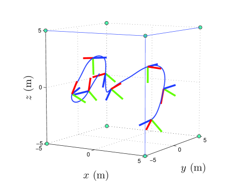
Figure 2: Position and attitude trajectory of the simulated vehicle.

The following two inertial directions, corresponding to nadir and Earth’s magnetic field direction, are measured by the inertial sensors on the vehicle:

$$d_{1}=[0\;\;0\;\;-1]^{\mbox{\small T}},\;\;d_{2}=[0.1\;\;0.975\;\;-0.2]^{\mbox{\small T}}.$$ (37)

For optical measurements, eight beacons are located at the eight vertices of the cube, labeled 1 to 8. The positions of these beacons are known in the inertial frame and their index (label) and relative positions are measured by optical sensors onboard the vehicle whenever the beacons come into the field of view of the sensors. Three identical cameras (optical sensors) and inertial sensors are assumed to be installed on the vehicle. The cameras are fixed to known positions on the vehicle, on a hypothetical horizontal plane passing through the vehicle, 120^∘ apart from each other, as shown in Fig. 1. All the camera readings contain random zero mean signals whose probability distributions are normalized bump functions with width of $0.001$m. The following are selected for the positive definite estimator gain matrices:

$$J =\mbox{diag}\big{(}[0.9\;\;0.6\;\;0.3]\big{)},$$

$$M =\mbox{diag}\big{(}[0.0608\;\;0.0486\;\;0.0365]\big{)},$$ (38)

$$\mathbb{D}_{r} =\mbox{diag}\big{(}[2.7\;2.2\;1.5]\big{)},\mathbb{D}_{t}=\mbox{diag}\big{(}[0.1\;\;0.12\;\;0.14]\big{)}.$$

$\Phi(\cdot)$ could be any $C^{2}$ function with the properties described in Section 3, but is selected to be $\Phi(x)=x$ here. The initial state estimates have the following values:

$$\begin{split}\hat{\mathsf{g}}_{0}&=I,\;\;\;\hat{\Omega}_{0}=[0.1\;\;0.45\;\;0.05]^{\mbox{\small T}}\mbox{ rad/s},\\ \mbox{ and }\hat{\nu}_{0}&=[2.05\;\;0.64\;\;1.29]^{\mbox{\small T}}\mbox{ m/s}.\end{split}$$ (39)

A conic field of view (FOV) of 2$\times$40^∘ is assumed for the cameras, which guarantees at least three beacons observed are common between successive measurements. The vehicle’s velocity vector is calculated from (28). The discrete-time estimator (30)-(34) is simulated over a time of $T=20$ s with time stepsize $\Delta t=0.02$ s. At each measurement instant, (30) is solved using Newton-Raphson iterations to find an approximation for $F_{i}$. The remaining equations (all explicit) are solved consecutively to generate the estimated states. The principal angle of the attitude estimation error and the position estimate error are plotted in Fig. 3. The angular and translational components of the vehicle’s velocity estimate errors are also depicted in Fig. 4.

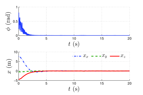
Figure 3: Principal angle of the attitude and position estimation error for CASE 1.

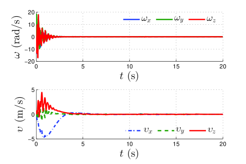
Figure 4: Angular and translational velocity estimation error for CASE 1.

6 CONCLUSION

This article proposes an estimator for rigid body pose and velocities, using optical and inertial measurements by sensors onboard the rigid body. The sensors are assumed to provide measurements in continuous-time or at a sufficiently high frequency, with bounded noise. An artificial kinetic energy quadratic in rigid body velocity estimate errors is defined, as well as two fictitious potential energies: (1) a generalized Wahba’s cost function for attitude estimation error in the form of a Morse function, and (2) a quadratic function of the vehicle’s position estimate error. Applying the Lagrange-d’Alembert principle on a Lagrangian consisting of these energy-like terms and a dissipation term linear in velocities estimation error, an estimator is designed on the Lie group of rigid body motions. A discrete-time counterpart of this estimator is also presented. In the presence of measurement noise, numerical simulations show that state estimates converge to a bounded neighborhood of the true states.

References

- [1] Bayadi, R., & Banavar, R. N. (2014). Almost global attitude stabilization of a rigid body for both internal and external actuation schemes. European Journal of Control, 20(1), 45–54.
- [2] Bonnabel, S., Martin, P., & Rouchon, P. (2009). Nonlinear symmetry-preserving observers on Lie groups. IEEE Transactions on Automatic Control, 54(7), 1709–1713.
- [3] Goodarzi, F. A., Lee, D., & Lee, T. (2013). Geometric nonlinear PID control of a quadrotor UAV on SE(3). In Proceedings of the European Control Conference (pp. 3845–3850). Zurich, Switzerland.
- [4] Goodarzi, F. A., Lee, D., & Lee, T. (2014). Geometric Adaptive Tracking Control of a Quadrotor UAV on SE(3) for Agile Maneuvers. ASME Journal of Dynamic Systems, Measurement and Control, 137(9), 091007.
- [5] Grip, H. F., Fossen, T. I., Johansen, T. A., & Saberi, A. (2015). Globally exponentially stable attitude and gyro bias estimation with application to GNSS/INS integration. Automatica, 51, 158–166.
- [6] Izadi, M., Samiei, E., Sanyal, A. K., & Kumar, V. (2015). Comparison of an attitude estimator based on the Lagrange-d’Alembert principle with some state-of-the-art filters. In Proceedings of the IEEE International Conference on Robotics and Automation (pp. 2848–2853). Seattle, WA, USA.
- [7] Izadi, M., & Sanyal, A. K. (2014). Rigid body attitude estimation based on the Lagrange-d’Alembert principle. Automatica, 50(10), 2570–2577.
- [8] Izadi, M., & Sanyal, A. K. (2015). Rigid body pose estimation based on the Lagrange-d’Alembert principle. To appear in Automatica.
- [9] Khalil, H. K. (2001). Nonlinear Systems (3rd edition). Prentice Hall, Upper Saddle River, NJ.
- [10] Khosravian, A., Trumpf, J., Mahony, R., & Lageman, C. (2015). Observers for invariant systems on Lie groups with biased input measurements and homogeneous outputs. Automatica, 55, 19–26.
- [11] Leishman, R. C., McLain, T. W., & Beard, R. W. (2014). Relative navigation approach for vision-based aerial GPS-denied navigation. Journal of Intelligent & Robotic Systems, 74(1-2), 97–111.
- [12] Mahony, R., Hamel, T., & Pflimlin, J. M. (2008). Nonlinear complementary filters on the special orthogonal group. IEEE Transactions on Automatic Control, 53(5), 1203–1218.
- [13] Marsden, J. E., & West, M. (2001). Discrete mechanics and variational integrators. Acta Numerica, 10, 357–514.
- [14] Misra, G., Izadi, M., Sanyal, A. K., & Scheeres, D. J. (2015). Coupled orbit-attitude dynamics and relative state estimation of spacecraft near small Solar System bodies. Advances in Space Research.
- [15] Mortensen, R. E. (1968). Maximum-likelihood recursive nonlinear filtering. Journal of Optimization Theory and Applications, 2(6), 386–394.
- [16] Rehbinder, H., & Ghosh, B. K. (2003). Pose estimation using line-based dynamic vision and inertial sensors. IEEE Transactions on Automatic Control, 48(2), 186–199.
- [17] Sanyal, A. K., Izadi, M., & Butcher, E. A. (2014). Determination of relative motion of a space object from simultaneous measurements of range and range rate. In Proceedings of the American Control Conference (pp. 1607–1612). Portland, OR, USA.
- [18] Shen, S., Mulgaonkar, Y., Michael, N., & Kumar, V. (2013). Vision-based state estimation and trajectory control towards aggressive flight with a quadrotor. In Proceedings of the Robotics Science and Systems.
- [19] Vasconcelos, J. F., Cunha, R., Silvestre, C., & Oliveira, P. (2010). A nonlinear position and attitude observer on SE(3) using landmark measurements. Systems & Control Letters, 59, 155–166.
- [20] Wahba, G. (1965). A least squares estimate of satellite attitude, Problem 65-1. SIAM Review, 7(5), 409.
- [21] Zamani, M. (2013). Deterministic Attitude and Pose Filtering, an Embedded Lie Groups Approach. Ph.D. Thesis. Australian National University, Canberra, Australia.