MAD-TH-15-07

Intersecting D3/D3’ system at finite temperature

William Cottrell, James Hanson, Akikazu Hashimoto,

Andrew Loveridge, and Duncan Pettengill

Department of Physics, University of Wisconsin, Madison, WI 53706, USA

We analyze the dynamics of intersecting D3/D3’ brane system overlapping in 1+1 dimensions, in a holographic treatment where $N$ D3-branes are manifested as anti-de-Sitter Schwartzschild geometry, and the D3’-brane is treated as a probe. We extract the thermodynamic equation of state from the set of embedding solutions, and analyze the stability at the perturbative and the non-perturbative level. We review a systematic procedure to resolve local instabilities and multi-valuedness in the equations of state based on classic ideas of convexity in microcanonical ensumble. We then identify a run-away behavior which was not noticed previously for this system.

1 Introduction

Recently in [1], a surprising subtelty was identified in a deceptively simple system of intersecting D-branes. Consider a system consisting of a D3 and a D3’ brane in type IIB string theory, oriented according to

0 1 2 3 4 5 6 7 8 9

D3 $$\circ$$

D3’

(1.1)

and separated by a finite distance in the $x_{9}$ direction.

Such a system preserves 8 supercharges. The low energy open string degrees of freedom can easily be enumerated as consisting of

1. An ${\cal N}=4$ $d=4$ $U(1)$ gauge theory living on D3

2. An ${\cal N}=4$ $d=4$ $U(1)^{\prime}$ gauge theory living on D3’

3. Two sets of hypermultiplets $B$ and $C$, arising from ${\cal N}=2$ $d=4$ hypermultiplets, dimensionally reduced to $d=1+1$ dimensions and charged as a bi-fundamental under $U(1)\times U(1)^{\prime}$

Explicit coupling between these states was worked out in [2]. This system, consisting entirely of D3 branes in type IIB string theory, is manifestly self-dual under $S$-duality.

On the first pass, there appears to be no obstruction to taking the zero slope limit $\alpha^{\prime}\rightarrow 0$ as long as one scales the distance separating the D3 branes to be of order

$$\Delta x_{9}=\alpha^{\prime}V$$ (1.2)

for some $V$ with dimension of mass. This then should give the mass of the $B$ and $C$ fields corresponding to the lowest energy 33’ strings.

As was pointed out in [1], this system exhibits a subtle paradox. A state with a single quantum of the $B$ or $C$ fields should exist as a BPS state in the spectrum of the theory, so its magnetic dual must also exist as a BPS state in order to be consistent with $S$-duality. Such a state should arise as a soliton of the field theory at hand. However, the soliton in question doesn’t appear to exist; something must therefore be wrong with the assumptions being made about the system.

The resolution proposed by [1] was that the zero slope limit failed to achieve decoupling. They then argued that a soliton does exist for a suitably modified effective field theory which contains singularities, signaling the need to include additional UV degrees of freedom. By considering full string theory as a UV completion, for instance, the effective field theory can be regularized, and the soliton can be constructed as the expected magnetic dual state.

Following the work of [1], a simple generalization in the brane construction was considered in [3]. This construction involved also scaling the angle between the D3-branes as $\theta\sim\alpha^{\prime}c$, introducing a new scale $c$ with dimension of mass squared. This gave rise to a tower of states of which $B$ and $C$ are the lightest [4]. In that setup, the decoupled theory in the zero slope limit is perfectly sensible, and supports the magnetic monopole soliton. One therefore learns that one can complete the effective field theory of [1] more economically than by invoking full string theory.

Taking the limit $c\rightarrow\infty$ while keeping $V$ fixed in the construction of [3] essentially amounts to recovering the naive zero slope limit considered in [1]. The techniques employed in [3] were not particularly effective for studying this limit, but in [5], we introduced another variation in the setup where we replaced the D3 with a stack of $N$ D3’s, so that we have as a gauge group $U(N)\times U(1)^{\prime}$. This allows us to analyze the system in a strong coupling limit where the $N$ D3-branes are replaced by their $AdS_{5}\times S_{5}$ dual, and the D3’ is treated as a probe. We then considered the magnetic soliton realized as a bion [6] melting into the horizon along the lines of [7]. It is then possible to see how in the $c\rightarrow\infty$ limit, the magnetically charged bionic soliton delocalizes and decouples as a normalizable state in the $c\rightarrow\infty$ limit.

The behavior of the D3/D3’ intersection is so counterintuitive that we probably have not yet seen the last word regarding this system. One direction which seems potentially interesting is to explore the thermodynamic behavior of this model. An elegant way to approach this issue incorprating the effects of interactions is to use gauge gravity correspondince, treating the D3’-brane as a probe, along the lines of [5]. Working in finite temperature then amounts to studying the embedding of a probe D3’-brane in an AdS-Schwartzschild background.

Problems of this type where a D$p^{\prime}$-brane probe is embedded into finite temperature D$p$-brane geometries have been considered extensively. Most of these works were in the context of exploring meson dynamics in holographic QCD [8, 9, 10, 11, 12, 13, 14, 15]. It was observed that these brane embeddings undergo a phase transition in which they penetrate the black hole horizon. This phase transtion was interpreted as “melting” of mesons, which was supported by subsequent analysis of the spectrum of fluctuations on the probe brane. The behavior near criticality for the melting transition also has a rich structure which was noticed even earlier in the context of domain walls [16, 17]. This analysis was carried out in various combinations of D$p$-brane background and D$p^{\prime}$-brane probes, and the general behavior of the system is dimension independent at least in a broad brush perspective.

In these class of problems, one generally enumerates the classical solutions to the equation of motion corresponding to static brane embedding configurations. The embeddings are characterized by a control parameter corresponding to quark mass, and have a definite order parameter corresponding to the quark condensate. The static solutions constrain the equation of state relating the quark condensate to quark mass. Treating these parameters as thermodynamic quantities, one can explore issues such as thermodynamic stability and hydrodynamic limits. Indeed, these system generally exhibits instabilities and multi-valued equation of states as were observed, for instance, in [18, 19, 20, 21].

The case of D3’-brane probe in the background of D3 branes oriented according to (1.1), however, is somewhat special. This is the case that was singled out in Reference [21] of [10]. There are two concrete senses in which the D3/D3’ system stands out. The brane embedding is characterized by a scalar on the D3’-brane world volume which happens to saturate the Breitenlohner-Freedman $m^{2}\geq-1$. [2]. As a result, the operators corresponding to these fields have scaling dimension

$$\Delta={d\mp\sqrt{d^{2}+4m^{2}}\over 2}=1$$ (1.3)

which is degenerate for $d=2$ and $m^{2}=-1$. This gives rise to logarithmic factors in the scaling of the embedding solution near the boundary, and exchange the roles of control and order parameters in the holographic dictionary as we will ellaborate further below. Also, the holographic renormalization procedure requires introducing an anomalous scale which can affect certain physical observables [22].

The thermodynamics of D3/D3’ system have been analyzed previously [23] although in that threatment, the control parameter of the embedding was treated as being fixed in defining the ensumble. The analysis of [23] was primarily focused on establishing the existence of a robust zero mode in the longitudional electric fluctuations and its implication for charge transport behaviors.

In this article, we re-examine the thermodynamics of D3/D3’ system with emphasis on understanding the thermodynamic stability issue of the quark condensate order parameter. We will explore the stability both at the perturbative and the non-perturbative level, and argue that the phase diagram of the system looks somewhat different than what was suggested in [23]. For now, we will focus primarily on zero charge embeddings. The extention of this analysis including charges and chemical potential will be reported in a separate publication.

2 D3’-brane probing finite temperature anti de Sitter space

In this section, we will review the analysis of embedding D3’-branes in the near horizon geometry of $N$ D3-branes at finite temperature. Similar analysis can be found extensively in the literature, but it is useful to formulate it here to make the notation and conventions explicit.

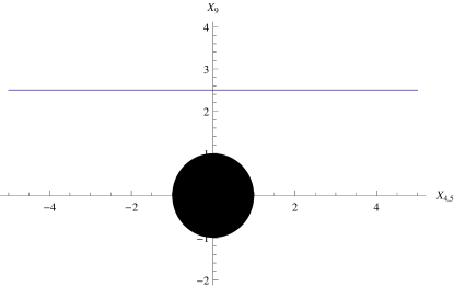
Figure 1: A schematic illustration of a flat brane embedding. This embedding is static in the absence of the black hole. We are interested in how this embedding is deformed when the black hole is introduced.

We begin by writing the supergravity solution corresponding to a stack of $N$ D3-branes at finite temperature in type IIB supergravity [24]

$$ds^{2}=-H^{-1/2}(-fdt^{2}+d\vec{x}^{2})+H^{1/2}(f^{-1}dr^{2}+r^{2}d\Omega_{5}^{2})$$ (2.1)

with

$$H=1+{R^{4}\over r^{4}},\qquad R^{4}=4\pi g_{s}N\alpha^{\prime 2}=\lambda\alpha^{\prime 2}\ ,$$ (2.2)

and

$$f=1-{r_{s}^{4}\over r^{4}}\ .$$ (2.3)

By standard arguments, the temperature $T$ and the horizon radius $r_{s}$ are related by

$$T={1\over\pi r_{s}\sqrt{H(r_{s})}}={U_{s}\over\pi\sqrt{\lambda}}.$$ (2.4)

We will take the decoupling limit by sending $\alpha^{\prime}\rightarrow 0$ keeping $U\equiv r/\alpha^{\prime}$ and $T$ fixed. This will also keep $U_{s}=r_{s}/\alpha^{\prime}$ fixed and finite.

At zero temperature, brane configuration oriented as (1.1) and illustrated in figure 1 is a consistent static solution. We are interested in how such an embedding is deformed when $T$ is no longer zero.

We will parameterize the six dimensions transverse to the $N$ D3-branes as

$$x_{4} = r\sin\theta_{1}\sin\theta_{2}\sin\theta_{3}\sin\theta_{4}\cos\theta_{5}$$ (2.5)

$$x_{5} = r\sin\theta_{1}\sin\theta_{2}\sin\theta_{3}\sin\theta_{4}\sin\theta_{5}$$ (2.6)

$$x_{6} = r\sin\theta_{1}\sin\theta_{2}\sin\theta_{3}\cos\theta_{4}$$ (2.7)

$$x_{7} = r\sin\theta_{1}\sin\theta_{2}\cos\theta_{3}$$ (2.8)

$$x_{8} = r\sin\theta_{1}\cos\theta_{2}$$ (2.9)

$$x_{9} = r\cos\theta_{1}\ .$$ (2.10)

We can then treat

$$t,\qquad z=x_{3},\qquad r,\qquad\phi=\theta_{5}$$ (2.11)

as the world volume coordinates in static gauge for the embedding, and denote

$$d^{4}\sigma=dt\,dz\,dr\,d\phi\ r$$ (2.12)

and treat $\theta_{1}$, $\theta_{2}$, $\theta_{3}$, and $\theta_{4}$ as parameterizing the embedding. We will restrict our attention to configurations where the gauge field on the world volume of D3’ is trivial at first. The system is invariant under $SO(4)$ rotational invariance acting on $(x_{6},x_{7},x_{8},x_{9})$, and it turns out to be dynamically consistent to set all but one of the four coordinates to zero. This is equivalent to setting

$$\theta_{2}=\theta_{3}=\theta_{4}={\pi\over 2}$$ (2.13)

and treating $\theta=\pi/2-\theta_{1}$ as the only relevant field variable. Restricting to embeddings which are invariant under translation in $t$ and $z$ directions, the resulting effective action is

$$S={1\over(2\pi)^{3}\alpha^{\prime 2}g_{s}}\int d^{4}\sigma\ \cos(\theta(r))\sqrt{1+r^{2}f(r)\theta^{\prime}(r)^{2}}\ .$$ (2.14)

Note in particular that the dependence on warp factor $H$ dropped out completely from the action.

In the zero slope limit, one sees that $\alpha^{\prime}$ scales out of the action

$$S_{DBI}={1\over(2\pi)^{3}g_{s}}\int d^{4}\Sigma\,\cos(\theta(U))\sqrt{1+\left(U^{2}-{U_{s}^{4}\over U^{2}}\right)\theta^{\prime}(U)^{2}}$$ (2.15)

with

$$d^{4}\Sigma=dt\,dz\,dU\,d\phi\,U\ .$$ (2.16)

For the purpose of finding the embeddings which extremizes this action, it is convenient to scale $U_{s}$ out by defining

$$u={U\over U_{s}}$$ (2.17)

so that the action takes the form

$$S={U_{s}^{2}\over(2\pi)^{2}g_{s}}\int d^{2}x\,du\,u\,\cos(\theta(u))\sqrt{1+\left(u^{2}-{1\over u^{2}}\right)\theta^{\prime}(u)^{2}}\,$$ (2.18)

where $L$ is the volume of the $x_{1}$ coordinate and $T$.

The task at hand now is to solve the equation of motion obtained by varying (2.18) which is a non-linear second order differential equation for $\theta(u)$ for $u$ taking values in the range $1\leq u\leq\infty$. For large values of $u$, $\theta(u)$ approaches zero and one can show that the solution can be parameterized in the form

$$\theta(u)=\left({c\log(u)\over u}+{m\over u}\right)$$ (2.19)

where we denote dimensionless integration constants $c$ and $m$ following the convention of [23]. Near $u=1$, we impose the regularity condition which constrains $c$ as a function of $m$.

The actual solutions satisfying these boundary conditions have to be obtained numerically. The general feature of the solutions we obtained is illustrated in figure 3. There are two different class of solutions depending on whether the brane penetrates the black hole horizon or not. The ones which do not, known as Minkowski embeddings, are illustrated in red. The ones which do, known as black hole embeddings, are illustrated in blue. Each of these solutions have a definite value of $c$ and $m$. The set of $(c,m)$ computed for these solutions are illustrated in figure 3.

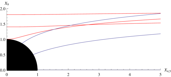
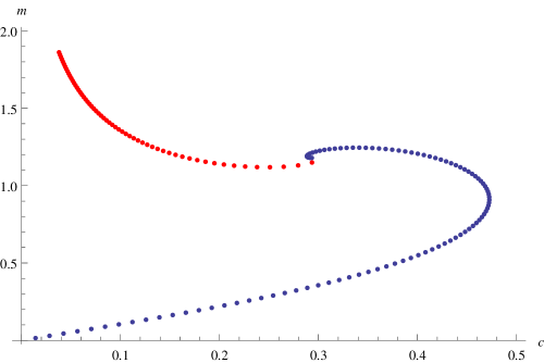
Figure 2: Black hole embedding illustrated in blue and Minkowski embeddedings illustrated in red.

Figure 3: $(c,m)$ for Minkowski (red) and black hole (blue) embeddings of D3’-probe. Each dot corresponds to numerical solutions we found with initial conditions for $\theta(U)$ specified either at the horizon $U=U_{s}$ for the black hole embeddings, or by fixing $\theta^{\prime}(U)$ at $\theta(U)=\pi/2$ for the Minkowski embeddings.

There are a number of features that are worth noting in figures 3 and 3. First, $m$ is not single valued as a function of $c$. Closely related is the fact that there is a maximum value of $c$ where $dc/dm=0$. Also, note that the embedding exhibits a self similar critical structure when the Mikowski and black hole embeddings meet. This was a feature originally noted [16, 17] and further ellaborated in the context of D$p$/D$q$ system in [10, 11]. It signals that there is a first order “meson melting” phase transition near the self-similar critical point. In this article, we will have more to say about the critical behavior at $dc/dm=0$ than at the self similar point.

3 Thermodynamics and Holography of D3/D3’ system

In this section, we elaborate on the thermodynamic and holographic interpretations of embedding solutions illustrated in figures 3 and 3.

First, it should be noted that all embeddings illustrated in figures 3 and 3 are asymptotically $AdS_{3}\times S_{1}$. The world volume degrees of freedom on D3’-brane will have a holographic interpretation as a field theory in 1+1 dimensions.

The embedding field $\theta(U)$ will be associated to an operator of dimension $\Delta=1$ to be associated with quark bilinar $\bar{\psi}\psi$ via the standard holographic dicationary which needs to be stated with some care because $\Delta$ is degenerate. Let us ellaborate on this matter further.

To interpret the system holographically, it is awkard to scale out $U_{s}$ since the holograhpic dictionary should be independent of $U_{s}$. Let us therefore parameterize the asymptotic behavior of the $\theta(U)$ in the form

$$\theta(U)={C\log(U/U_{*})\over U}+{M\over U}$$ (3.1)

where once again adapting the notation of [23], $C$ and $M$ have dimension of mass, whereas $U_{*}$ is an arbitrary scale with dimension of mass which one must introduce in order to make sense of the argument of the logarithm. An astute reader should notice at this stage that there is some ambiguity in how $M$ is defined since changing $U_{*}$ has the effect of shifting $M$. It would therefore be essential to understand if and how $U_{*}$ affects physical observables (or not.) Several related issues will arise in the discussion below and we will be doing due diligence to track these issues.

We begin by recalling the standard formulation of the holograhpic dictionary (see e.g. [25] for a review) that

$$Z_{bulk}[C(x)]=\langle e^{\int d^{d}x\,C(x){\cal O}(x)}\rangle_{boundary}$$ (3.2)

where the left hand side of the equality describes a path integral for bulk fields such as $\theta(U)$ carried out in such a way that $\theta(U)$ asymptotes to

$$\theta(U)\sim{C(x)\log(U/U_{*})\over U}$$ (3.3)

as the boundary is approached by taking $U\rightarrow\infty$. This path integral and boundary condition as formulated is independent of $U_{*}$. One might formulate the right hand side for the $\theta(U)$ field to take the form

$$Z_{bulk}[C(x)]=\int[D\theta(U,x)]_{C(x)}e^{-S_{DBI}[\theta(U,x)]}$$ (3.4)

where $S_{DBI}$ is the action given in (2.15), and the boundary condition for $\theta(U)$ is referenced implicitly in the specification of the measure. One can apply the saddle point approximation to identify the domimant contribution to this path integral, which simply amounts to evaluating the action for the solution to the equations of motion enumerated in figures 3 and 3. As is typical in these computation, however, the action formally diverges, and a renormalization is required to define the bulk side of the correspondence unambiguously. For the D3/D3’ system, this was worked out explicitly in (6.2)–(6.4) of [22]. We are simply instructed to add the holographic renormalization counter-term

$$S_{CT}=\left.{1\over(2\pi)^{2}g_{s}}\int d^{2}x\,U^{2}\left(-{1\over 2}+{1\over 2}\left(1-{1\over\log(U/U_{CT})}\right)\theta(U)^{2}\right)\right|_{U=U_{UV}}\ .$$ (3.5)

With this counter-term included,

$$Z_{bulk}[C(x)]=\int[D\theta(U,x)]_{C(x)}e^{-(S_{DBI}[\theta(U,x)]+S_{CT}[\theta(U,x)])}$$ (3.6)

where $U_{UV}$ is the ultra-violet cut-off scale, whereas $U_{CT}$ is a new scale that is required in order to make the logarithm appearing in the counter-term make sense. This expression is finite in the $U_{UV}\rightarrow\infty$ limit. However, the dependence on $U_{CT}$ which characterizes the renormalization scheme survives and should a priori be treated as independent of $U_{*}$ and $U_{s}$. A useful feature to isolate in the holographic dictionary is the prescription to extract the expectation value of the operator dual to $\theta(U)$. This is to be derived by varying the logarithm of $Z[C(x)]$ with respect to $C(x)$. By manipulating $S_{DBI}+S_{CT}$, one finds that

$$\langle{\cal O}(x)\rangle=-{1\over(2\pi)^{2}g_{s}}(M(x)-C(x)\log(U_{*}/U_{CT}))\ .$$ (3.7)

It is also useful to infer the values of $(C,M)$ for the solutions enumerated in figures 3 and 3 which are parameterized in terms of $(c,m)$. By simply relating (2.19) to (3.1), we find that

$$C=U_{s}c,\qquad M=U_{s}\left(m-c\log(U_{s}/U_{*})\right)\ .$$ (3.8)

In terms of $(c,m)$, we can write

$$\langle{\cal O}(x)\rangle=-{1\over(2\pi)^{2}g_{s}}U_{s}(m-c\log(U_{s}/U_{CT}))$$ (3.9)

whose significance is the fact that the dependence on $U_{*}$ has dropped out. However, the dependence on $U_{s}$ and $U_{CT}$ remains.

At this point, we can also compute the free energy by evaluating the action with time compactified on a circle of radius $1/2\pi T$

$$G(C,T)=-T\log(Z[C])$$ (3.10)

or by computing

$$G(C,T) = -{L\over(2\pi)^{2}g_{s}}\int_{0}^{C}dC^{\prime}(M(C)-C^{\prime}\log(U_{*}/U_{CT}))$$ (3.11)

$$= -{LU_{s}^{2}\over(2\pi)^{2}g_{s}}\int_{0}^{c}dc^{\prime}(m(c)-c^{\prime}\log(U_{s}/U_{CT}))$$ (3.12)

which gives an equivalent $U_{*}$ independent result. Since $U_{*}$ is essentially unphysical, it is conveninet to set $U_{*}=U_{CT}$ so that

$$\langle{\cal O}(x)\rangle={1\over(2\pi)^{3}g_{s}}M$$ (3.13)

for the remainder of this paper.

We are also now in the position to display thermodynamic data such as the equation of state $M(C,T)$ and the free energy $G(C,T)$ for various fixed values of $T/U_{CT}$. Few examples are illustrated in figures 4.

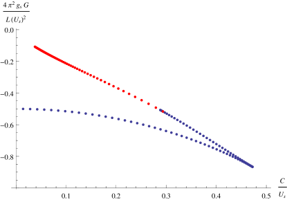
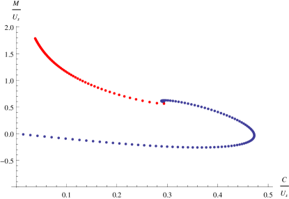
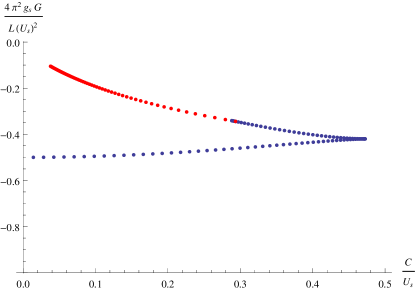
Figure 4: $M(C,T)$ and $G(C,T)$ as a function of $C$ for $\log(U_{s}/U_{CT})=-2$ (top) and $\log(U_{s}/U_{CT})=2$ (bottom)

It is also straight forward to infer quantity such as

$$S(C,T)=-\left.{\partial G\over\partial T}\right|_{C}={LU_{s}\over(2\pi)^{2}g_{s}}\left(2\int_{0}^{c}m(c)dc^{\prime}-cm-{1\over 2}c^{2}\right)$$ (3.14)

which happens to be independent of $U_{CT}$ and plot it as a function of $T$ with $C$ fixed. We illustrate that in figure 5. This is essentially equivalent to what is illustrated in figure 3.d of [23] except that we do not find any evidence of the dotted part of their graph. This view is supported also from the structure of equation of state illustrated in figure 3 which has exactly two, not three, branches as $c$ approaches zero. We will ellaborate further on this point below.

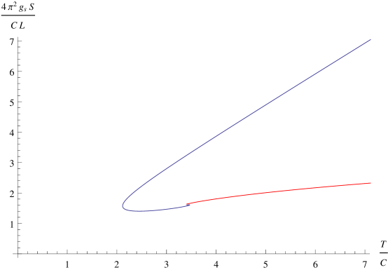
Figure 5: $S(C,T)$ as a function of $T$ for fixed $C$. This curve turns out to not depend on $U_{CT}$.

4 Physical interpretation of D3/D3’ thermodynamics

In the previous section, we outlined the general features of the D3/D3’ system which can be presented in the thermodynamic context. The control and order parameters, $(C,M)$ play a role very similar to mechanical parameters $(P,V)$, magnetic parameters $(H,M)$, etc., up to a sign which arises from conventions which are set for historical reasons.

There are two notable features about the equation of state and the subsequent thermodynamics summarized in the previous section. One is the fact that the scale $U_{CT}$ affects the equation of state which is physically observable. The other is the fact that the equation of state exhibits multi-valued-ness and regions of instability. This latter issue is somewhat familiar from previous consideration of black hole thermodynamics [18, 19, 20, 21]. It is generally stated that the van der Waals model of liquid-gas phase transition is a prototype for understanding these issue. Nonetheless, in the context of van der Waals model, it was the order parameter as a function of the control parameter, $V(P)$ that was multi-valued, whereas in the case of D3/D3’ system, it is exactly the opposite. Another apparent paradox stems from the fact that the sucsceptiblity

$$\chi_{\theta}={dC\over dM}$$ (4.1)

characterizing this system is explicitly dependent on $U_{CT}$ whereas dymamical features such as the poles of quasi-normal modes at fixed control parameter $C$ are manifestly independent of $U_{CT}$. The goal of this section is to clarify these issues.

Let us begin by recalling the classical thermodynamic perspective on stability. A useful quantity to consider is the effective potential of the order parameter obtained by Legendre transforming the free energy

$$F(M)=\left.G(C)+{L\over(2\pi)^{2}g_{s}}CM\right|_{G^{\prime}(C)=-M}\ .$$ (4.2)

One can also compute $F(M)$ in terms of the equation of state

$$F(M)={L\over(2\pi)^{2}g_{s}}\int^{M}dM^{\prime}C(M^{\prime})$$ (4.3)

Plotted as a function of $M$ with fixed values of $\log(U_{s}/U_{CT})$, they take the form illustrated in figure 6. For all of these figures, $M\rightarrow\infty$ corresponds to the Minkowski branch, and $F(M)$ approaches a constant, reflecting the fact that the area under the curve $C(M)$ is finite.

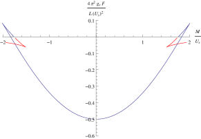
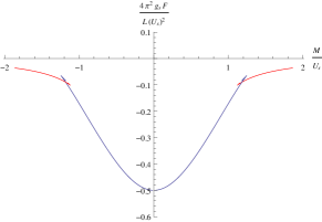
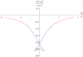
Figure 6: $F(M)$ for $\log(U_{s}/U_{CT})$ taking values $-2$ (left), $0$ (center), and $2$ (right). For all of these cases, $F(M)$ asymptotes to a constant value 0 as $M$ is taken to infinity.

The free energy $F(M)$ is an important physical quantity characterizing the effective thermodynamic behavior of the order parameter $M$. If a system with free energy $F(M)$ is brought to contact with a reservoir with which the $M$-ness is freely exchanged, the system will achieve equilibrium when $M$ minimizes the potential

$$F_{eff}(M)=F(M)-{L\over(2\pi)^{2}g_{s}}C_{ext}M$$ (4.4)

where $C_{ext}$ is the control parameter conjugate to $M$ of the reservoir. One of course recognizes

$$G(C_{ext})=\left.F(M)-{L\over(2\pi)^{2}g_{s}}C_{ext}M\right|_{F^{\prime}(M)-C_{ext}=0}$$ (4.5)

as the conjugate Gibbs Free energy when the $M$ that minimizes $F_{eff}(M)$ is substituted into $F_{eff}(M)$. From that point of view, it is natural to associate the susceptibility

$$\chi_{\theta}={(2\pi)^{2}g_{s}\over L}F^{\prime\prime}(M)={dC\over dM}$$ (4.6)

as parameterizing the stability of the system. The susceptibility $\chi_{\theta}$ is dependent on $U_{CT}$.

Let us now take a closer look at the form of $F(M)$ illustrated in figure 6 and make several observations.

1. $F(M)$ is multi-valued over some range of $M$.

2. The susceptibility $\chi_{\theta}$ at $M=0$ (as well as other values of $M$) changes as $U_{s}/U_{CT}$ is varied, and can get negative, signalling an instability, for instance for large positve values of $\log(U_{s}/U_{CT})$.

3. The effective action $F_{eff}(M)$ is not concave everywhere and does not have global stable minima when $C_{ext}$ is non-vanishing.

Let us address each of these observations more carefully.

4.1 Multi-valuedness of $F(M)$

This issue is not too serious. The fact that there are multiple branches for some fixed value of $M$ (and $T$) simply reflects the fact that there are multiple thermodynamic states corresponding to these order and fixed parameters. However, in thermodynamics, one focuses on the dominant state in the ensumble, which is the one with the lowest free energy. So in reading figure 6, one should simply trace the branch with smallest $F(M)$ for any fixed value of $M$, regardless of the discontinuities that might result.

4.2 Susceptibility and its dependence on $U_{CT}$

This is an extremely important yet subtle issue. Taken at face value, it implies that the susceptibility and therefore the thermodynamic stability depends on $U_{CT}$. For example, in figure 6, we see for $\log(U_{s}/U_{CT})=2$ that $F(M)$ is concave down indicating instability at $C=M=0$.

On the other hand, it is generally established that the thermodynamic stability can be inferred from the presence or absence of poles of quasi-normal modes in the upper half of the complex $\omega$ plane [27]. The quasi-normal mode analysis, however, does not depend on holographic renormalization counter-term. As such, it would appear that thermodynamic stability is independent of $U_{CT}$. But this is in direct contradiction with what we stated in the previous paragraph.

The eventual resolution of this apparent tension can be understood as susceptibility being dependent on $U_{CT}$ but not the stability. But there are number of subtleties involved in arriving at this conclusion which we will describe in this subsection.

The issue boils down to mapping out the allowed range of values in enumerating the renormalization schemes which $U_{CT}$ is parameterizing. On the other hand, $\chi_{\theta}(M=0)$ depends on $U_{CT}$ and as such can also be considered as parameterizing the renormalizaiton schemes. The susceptibiltiy $\chi_{\theta}(M=0)$ however is a quantity that is easy to measure. $U_{CT}$, on the other hand, is an abstract quantity appearing in the counter-term which can only be inferred by measuring some physical quantity (such as $\chi_{\theta}(M=0)$) and using its relationship to $U_{CT}$. The choice to parameterize the renormalization scheme with $\chi_{\theta}$ at $M=0$ is an arbitrary choice. Any other $M$ can be used as a reference. The situation is analogous to the relation between renormalized coupling in $\overline{MS}$ scheme and physical coupling inferred from scattering at some definite energy. The former is the analogue of $U_{CT}$ whereas the latter is the analogue of $\chi_{\theta}(M=0)$.

The question then is what constitutes the appropriate range of parameters to enumerate distinct renormalization scheme. Should it be $0\leq U_{CT}\leq\infty$, or $-\infty\leq\chi_{\theta}(M=0)\leq\infty$? To the extent that $\chi_{\theta}(M=0)$ is the physical parameter, it would seem natural to treat the latter as parameterizing physically distinct renormalization schemes. We will adopt that point of view in this paper. There is a possibliy that extrapolation beyond infinite $\chi_{\theta}(M=0)$ would admit interpretation along the lines of dualities where one extrapolates beyond infinite coupling, but we will not pursue that possiblity in this paper.

This implies however that the behavior illustrated in figure 4 and 6 for $\log(U_{s}/U_{CT})=2$ where the $\chi_{\theta}(M=0)$ is negative signalling instability corresponds to pushing $\chi_{\theta}(M=0)$ beyond infinity and should be excluded from our analysis. At $M=0$, one can explore the full range of $0<\chi_{\theta}(M=0)<\infty$ by letting $U_{s}/U_{CT}$ vary. Susceptibility at $M=0$ for this system is always positive.

This however does not imply that the system is always stable or that the stability analysis is completely unrelated to the quasi-normal mode analysis. To see this, suppose we set the temperature $U_{s}=U_{CT}$ so that the equation of state is given by what is illustrated in figure 3. For every $0<C<C_{max}$, there is a subleading branch of solutions where

$${dC\over dM}<0\ .$$ (4.7)

One can see the same thing by looking at unstable stationary point in the potential illustrated in figure 6 which is appropriately tilted by the inclusion of $-C_{ext}M$ term as is illustrated in fugre 7. One exepcts to find a corresponding pathology in the spectrum of quasi-normal modes for the fluctations around such unstable background solutions, but how can one understand its appearance short of doing an explicit computation?

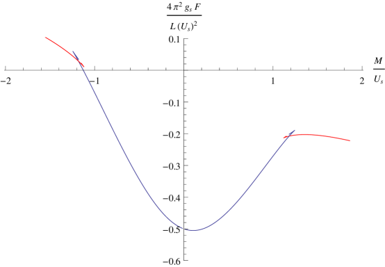
Figure 7: $F_{eff}(M)=F(M)-C_{ext}M$ with $C/U_{s}=0.1$.

One way to see that a cross-over into unstable behavior is taking place is to focus on the state at $C=C_{max}$ where $\chi_{\theta}=dC/dM=0$. Recall that for every point on figure 3 there is a corresponding solution $\theta(U)$ which extremizes the action (2.15). If we parameterize these solutions for fixed value of $M$ by $\theta_{M}(U)$, then at $M=M_{crit}$ corresponding to $C=C_{max}$, it follows that

$$\psi(U)=\left.{d\over dM}\theta_{M}(U)\right|_{M=M_{crit}},$$ (4.8)

$\psi(U)$ is a gap-less quasi-normal mode with $\omega=k=0$. The fact that a gapless mode is appearing precisely when the susceptibility $\chi_{\theta}=0$ strongly suggests that an unstable pole would appear upon continuing to the branch where the susceptibility is negative. This cross-over across $\chi_{\theta}=0$ is different from crossin over $\chi_{\theta}=\infty$ which we discussed earlier in the context of placing a bound on $U_{CT}$.

By a similar token, for sufficiently large negative value of $\log(U_{s}/U_{CT})$, we encounter a point in the unstable branch where $\chi_{\theta}$ reaches negative infinity. This can be seen in figure 4 where the tangent of $M(C)$ is horizontal. For $\log(U_{s}/U_{CT})=-2$, this point corresponds to the switch back point in the black hole embedding branch illustrated on the left most figure of 6. This issue is somewhat academic, however, since the switch back point is already subdominant in the saddle point approximation as can be seen in figure 6.

The critical point $(C,M)=(C_{max},M_{crit})$, on the other hand, is a dominant saddle point and as such the resulting critical behavior giving rise to a new channel for dissipating energy in the hydrodynamics limit near that point is a real physical feature of this model, at least at the perturbative level. This critical point can also be seen to correspond to the point in figure 5 where $T=T_{min}$ takes on a minimal value. The entropy $S$ plotted as a function of $T$ in figure 5 is double valued. From the thermodynamic point of view, the dominant branch, however, is naturally the one with greater entropy. So, the black hole embedding dominates, and the Minkowski embedding is the subdominant one. For $T>T_{min}$, the system naively seems to be perfectly stable and well behaved. At $T=T_{min}$, there is a critical behavior. The phase strucure implied by these features are consistent with the $d=0$ slice of the phase digram illustrated in figure 4 of [23]. This however raises one obvious question. If at $T=T_{min}$ we encounter a crticial behavior, where does the system equilibriate to for $T<T_{min}$. In order to address this issue, we need to go beyond the scope of perturbative stability analysis, and consider the global issues. We will discuss that issue in the next subsection.

The apparent quantitative mismatch in the dependence of $U_{CT}$ between susceptibility and quasi-normal mode specturm can also be seen in the computation of correlators in the real-time formalism. The retarded Greens function is computed using the prescription given in equation (3.15) [28]

$$G^{R}(k)=-2{\cal F}(k,z)|_{z_{B}}=\sqrt{-g}g^{zz}f_{-k}(z)\partial_{z}f_{k}(z)$$ (4.9)

for a suitably normalized ingong wave $f(z)$, where $z\sim 1/u$. However, strictly speaking, ${\cal F}$ is divergent for our model and a counter-term is needed to render this expression finite.

One can understand the origin of this divergence as arising from computing the two ponit function of operator whose dimension is $\Delta$ so that at short distance, it scales as

$$G(k)=\langle{\cal O}(x){\cal O}(0)\rangle\sim{1\over x^{2\Delta}}$$ (4.10)

which then in momentum space takes the form

$$G(k)\sim{1\over k^{d-2\Delta}}$$ (4.11)

for large $k$. The issue arises when $d-2\Delta\leq 0$ so that this correlation funciton do not decay at large $k$. This is the case in our example because $d-2\Delta=0$. So strictly speaking, one expects the two point function to scale for large $k$ as [22]

$$G(k)\sim\log(k^{2}/\mu^{2})$$ (4.12)

for some scale $\mu$. We are however interested in the small $k$ behavior when the system is at finite temperature.

The two point function should then admit a spectral decomposition

$$G(k)=\int ds{\rho(s)\over k^{2}+s}$$ (4.13)

where by power counting, we know that $\rho(s)$ must asymptote to a constant at large $s$. The integral over $s$, however, does not converge and must be regulated, for instance, by adding a term

$$G(k)=\int ds\left({\rho(s)\over k^{2}+s}-{\rho(s)\over\Lambda^{2}+s}\right)=a_{0}+a_{2}k^{2}+a_{4}k^{4}+\ldots$$ (4.14)

The term added is a contact term in that it is independent of $k$. It only affects the $a_{0}$ term in the small momentum expansion of $G(k)$. The scale $U_{CT}$ and $\mu$ arises from these considerations, which does affect the two point function and therefore the susceptibility, but does not affect the pole structure of $G(k)$.. Nonetheless, both the susceptibility and the quasi-normal mode spectrum knows when the system is perturbatively unstable, and exhibits the appropriate symptoms.

4.3 Non-perturbative stability of the D3/D3’ system

In this section, we will discuss the subject of how the unstable states relaxes to the true equilibrium state. This issue requires consideration beyond the perturbative analysis, but the subject is not an unfamiliar one. The same issue arises in the phase structure of liquid-gas transitions in the van der Waals model. Let us see how that applies to the D3/D3’ system under consideration.

It is a fundamental fact of statistical mechanics that the set of accessible states parameterized by the order parameters form a convex set. A nice historical review of this basic notion can be found in [26]. If one is working at fixed temperature $T$, in a system with a single order parameter $M$, the region bounded by the curve $F(M)$ must be convex, or equivalently, $F^{\prime\prime}(M)>0$. But sometimes, as is the case here, by working out the equation of states for what one believes is the dominant thermodynamic configuration, one finds regions where $F^{\prime\prime}(M)$ is negative, signalling an instability. For our system, this can be seen very explicitly in figure 6 where $F(M)$ is concave down for large values of $M$. Equivalently, one can see regions where $dC/dM$ is negative in the equation state illustrated in figure 3 and 4.

The standard procedure when this happens is to observe that the system can acheve a state with lower free energy for fixed $M$ by being in a hetrogeneous co-existence state. A co-existence of two state will give rise to a configuration with $(M,F(M))$ interpolating between the pair of states. As a result, the maximal extension of the space of states allowed by considering co-existence states is precisely the convexification of $F(M)$ achieved by supplementing $F(M)$ with “ruled surfaces” in the terminology of [26].

This is exactly what happens to the equation of state in van der Waals system. We illustrate the standard diagram displaying a collection of isothermal $P(V)$ curve in figure 8. The point to note is the fact that 1) there are regions where $-dP/dV<0$ signalling instability, and 2) that this gives to a modified equation of state by allowing coexistence states. It should also be emphasized that 3) the region of phase diagram modified by allowing coexistence regions (shaded blue region in figure 8) are strictly greater than the region where the system exhibts apparent instability (shaded red region in figure 8).

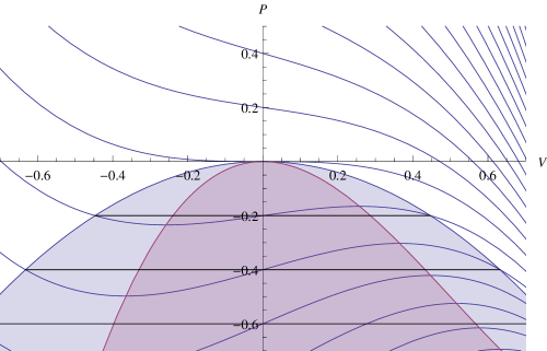
Figure 8: Typical equation of state $P(V)$ for various fixed $T$ illustrating thermodynamic instability, coexistence of states, and the critical point. As $T$ is varied, regions of instability where $-\left.dP/dV\right|_{T}<0$ appears and is shaded in red. This causes the system to undergo a first order phase transition where the equation of motion is modified by the ruled coexistence line, illustrated in black. The coexistence region is generally larger than the unstable region. So the local instability in the red shaded region affects the equilibrium configuration of all points in the $(P,V)$ region inside the blue shaded region.

How do these ideas apply to the D3/D3’ system? From the equation of state illustrated in figures 3 and 4 where $C(M)$ is rapidly approaching zero as $M$ is increased, it follows that $F(M)$ must approach a constant value (set to zero for convenience in figure 6.) As soon as this potential is slighlty tilted in response to non-vanishing external control parameter $C_{ext}$ as is illustrated in figure 7, the displaced local minima is no longer a global minima and the system is susceptible to decay via tunneling into a run away behavior towards large $M$. If $C_{ext}$ is taken to be larger than $C_{max}$, even the local minima disappears and the potential does not have any stationary points. (The situation is a little different when the some net charge is introduced to the D3’-brane world volume. We will ellaborate further on this case in a separate publication.)

From the point of view of convexifying $F(M)$, we see that the result is to say

$$F(M)=F(M=0)=\mbox{constant}$$ (4.15)

which is even more susceptible to runaway behavior when $C$ is non-vanishing.

What appears to be happening is that the $d=0$ slice of the phase diagram illustrated in figure 4 of [23] degenerated completely and that at finite $C$, the system is completely unstable at the non-perturbative level.

What this means, presumably, is that the classical treatment is predicting its own thermodynamic demise and that some configuration not presently accounted for will modify the equation of state to provide the stable, equilibirium state for this system. Such corrections, however, must arise from string or quantum corrections and is expected to scale non-trivially with respect to $g_{S}$ and $N$. It is possible that such correction would also give rise to the branch drawn with dotted lines in figure 3.d of [23].

Alternatively, the D3/D3’ system is intrinsically unstable. At this moment, we do not have any reason to rule out that possiblity.

In this article, we took the boundary of $AdS_{5}\times S_{5}$ to be flat and infinite in volume. It would be interesting to repeat this analysis treating the boundary to be a $S_{3}$ of finite size. In that case, the entire system undergoes a Hawking-Page transition [30], giving rise to a qualitatively new behavior also for the D3’-brane embedding. It is somewhat unexpected, however, for thermodynamic stability of a system to rely on finite volume issue. In any case, it would be very interesting to understand all the different ways in which the run-away behavior seen in this system can be stablized.

5 Discussions

In this article, we analyzed the embeddings of D3’-brane probe in Schwarzschild $AdS_{5}$ geometry and studied their thermodynamic interpretations, with emphasis on order parameter and control parameter dual to the brane probe embedding psuedo scalar field $\theta(U,x)$. We described the subtle relationship between the anomalous scale $U_{CT}$ introduced in the holographic renormalizatoin procedure, thermal susceptibitliy $\chi_{\theta}$, and the spectrum of quasi-normal modes.

The resulting analysis of the theromdynamic stability revealed that while the system is perturbatively stable for some range of parameters, it is unstable at the non-perturbative level almost everywhere. The full implication of this instability is not completely clear to us at the moment. It should be noted that our consideration was limited to treating the branes in the probe approximation. Perhaps gravitational back reaction will stabilize the system, although properly addressing this issue is a tall order for an intersecting brane system. It is also possible that a satisfactory resolution will require going beyond the semi-classical treatment of these systems.

The original goal of this study was to find some relation between subtle features of the thermodynamics of D3/D3’ brane system to the subtle features discussed recently by Mintun, Polchinski, and Sun [1]. At the moment, the only connection we see is the fact that some of the pathologies are due to low co-dimension physics in both instances. We hope to provide more insight into this issue in the future.

Finally, let us comment that the intersecting D3/D3’ system could also prove to be useful as a probe of the region behind the horizon in the context of entanglement entropy where the degrees of freedom crossing the horizon is in the open string sector [31]. Just like in other attempts to probe behind the horizon such as [32, 33], we expect the sensitivity of probe dyanmics to behind the horizon physics to be highly suppressed. Nonetheless, perhaps something can be gained by using an open string probe instead of a closed string probe.

Appendix A More on embeddings

In this appendix, we offer an alternative parameterization of the equation of motion (2.15) where we map the problem to dynamics of a particle rolling down a potential. This formulation is useful for visualizing the solutions and for providing assurance that all solutions are accounted.

The procedure to convert (2.15) into the classical potential problem form is essentially the same steps one takes to convert the Nambu-Goto action in to the Polyakov action form. This can be done by introducing an auxiliary world volume parameter $\tau$ and a Lagrange multiplier $\lambda(\tau)$ and re-writing the effectively one dimensional form of (2.15) as

$$\int d\tau\ {1\over 2}U(\tau)\cos(\theta(\tau))\left[\lambda(\tau)^{-1}(U^{\prime}(\tau)^{2}+(U(\tau)^{2}-U_{s}^{4}U(\tau)^{-2})\theta^{\prime}(\tau)^{2})+\lambda(\tau)\right]\ .$$ (A.1)

Solving for the Lagrange multiplier and setting $\tau=U$ recovers (2.15). On the other hand, imposing as the gauge condition

$$\lambda(\tau)={U^{2}-U_{s}^{4}U^{-2}\over U_{s}^{2}}U\cos\theta\ ,$$ (A.2)

setting

$$U^{2}=U_{s}^{2}\cosh s\ ,$$ (A.3)

and rescaling $\tau=U_{s}\sigma$ will scale out $U_{s}$, leads to

$$L=U_{s}^{2}\int d\sigma\ {1\over 2}\dot{s}^{2}+{1\over 2}s^{2}\dot{\theta}^{2}+{1\over 2}\sinh^{2}s\cos^{2}\theta$$ (A.4)

where $s$, $\theta$, and $\sigma$ are dimensionless, and dot denotes derivative with respect to $\sigma$. In the form (A.4) the problem is essentially that of a particle whose positions are parameterized by $1<s<\infty$ and $-\pi/2<\theta<\pi/2$ rolling along a potential

$$V(s,\theta)=-{1\over 2}\sinh^{2}s\cos^{2}\theta\ .$$ (A.5)

Reparameterization invariance further implies that the solution should correspond to trajectory with vanishing Hamiltonian

$${\cal H}=0\ .$$ (A.6)

A large class of solutions arises as a trajectory of a particle rolling up, turning around, and rolling back down the potential in $(s,\theta)$ coordinates (A.5) which we illustrate in figure 10. These are the worm hole embeddings in the terminology of [16, 17]. In the original $(X_{4,5},X_{9})$ cooridinates, they look like an embedding illustrated in figure 10. In the large $X$ region, these correspond to having both a brane and an anti-brane along the lines of [6, 34] and are not the solutions we are looking for.

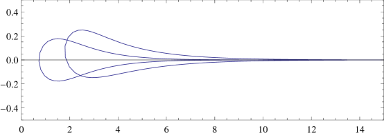
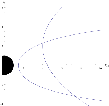
Figure 9: The trajectory of figure 10 in $(s,\theta)$ plane. The horizontal axis is $\log(s)$ and the vertical axis is $\theta/\pi$. The horizon corresponds to the left edge at $\log(s)=0$.

Figure 10: Some generic solutions to the embedding equation of a D3’-brane in a finite temperature $AdS_{5}\times S_{5}$ background. The full embedding is cylindrically symmetric with respect to rotation around the $X_{9}$ axis. The black disk represents the region behind the event horizon.

The only other possibility is for the trajectory in the $(s,\theta)$ plane to hit the boundary of the region on which the space is defined, i.e. $s=1$ for arbitrary $\theta$, or $\theta=\pi/2$ for arbitrary $s$. These solutions are referred to as the black hole and the Minkowski embeddings, respectively. These trajectories are specified uniquely by giving the starting position of the trajectory along the boundary of the $(s,\theta)$ plane because the quadratic term in the equation of motion inferred from (2.15) degenerates there.

The trajectory resulting from these initial conditions are illustrated in figure 11. The same solutions in the original $(X_{4,5},X_{9})$ coordinates is illustrated in figure 3. The trajectories starting at $s=1$ boundary are the black hole embedding, and the trajectories starting at $\theta=\pi/2$ are the Minkowski embedings.

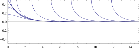
Figure 11: The trajectories of figure 3 in the $(s,\theta)$ plane. The horizontal axis is $\log(s)$ and the vertical axis is $\theta/\pi$.

Appendix B Retarded Green Function and Quasi-Normal Mode for $\theta(U)=0$ background

In this appendix, we will outline the computation of retarted Green function for the $\theta(U)$ fluctuation using the prescription of [28]. We start by generalizing (2.15) to include momentum and energy and write

$$S_{DBI}={1\over(2\pi)^{2}g_{s}}\int d^{2}x\,dU\,U\cos(\theta(U))\sqrt{\left(1+fU^{2}\right)\theta^{\prime}(U)^{2}+{\lambda(fk^{2}-\omega^{2})\over U^{2}}\theta(U)^{2}}\ .$$ (B.1)

In order to compute the retarded Green function, we need to expand $\theta(U)$ to quadratic order around a solution to the equation of motion. This is quite complicated for generic solution $\theta_{0}(U)$, but is tractable for the trivial solution $\theta_{0}(U)=0$. For that case, the linearized action reads

$$S_{lin}\sim{1\over 2}U\left(U^{2}f\theta^{\prime}(U)^{2}-\theta(U)^{2}+{\lambda(fk^{2}-\omega^{2})\over fU^{2}}\theta(U)^{2}\right)$$ (B.2)

The equation of motion resulting from this action can be written in a canonical form in terms of

$$\theta(x)=(x-1)^{1/2}y(x)\ ,\qquad x={U^{2}-U_{s}^{2}\over U^{2}+U_{s}^{2}}\,$$ (B.3)

with

$$\omega={U_{s}w\over\sqrt{\lambda}},\qquad k={U_{s}q\over\sqrt{\lambda}}$$ (B.4)

so that the equation of interest is expressed as

$$0 = y^{\prime\prime}(x)-\left({1\over 1-x}-{1-iw/2\over x}\right)y^{\prime}(x)$$ (B.6)

$$+\left(\frac{k^{2}-w^{2}+2}{8(x-1)}+\frac{-2q^{2}+w^{2}-2}{8x}+\frac{k^{2}}{8(x+1)}+\frac{w^{2}}{16x^{2}}\right)y(x)\ .$$

For non-zero $q^{2}$, this equation has four singular points at $x=0$, $x=1$, $x=-1$, and $x=\infty$, and as such is not analytically tractable. But when $q^{2}=0$, the singularity at $x=-1$ goes away, and one arrives at a hypergeometric equation solved by

$$y(x) = c_{1}(-1)^{-\frac{iw}{4}}x^{-\frac{iw}{4}}\,_{2}F_{1}\left(\frac{1}{2}-\left(\frac{1}{4}+\frac{i}{4}\right)w,\left(\frac{1}{4}-\frac{i}{4}\right)w+\frac{1}{2};1-\frac{iw}{2};x\right)$$ (B.8)

$$+c_{2}(-1)^{\frac{iw}{4}}x^{\frac{iw}{4}}\,_{2}F_{1}\left(\frac{1}{2}-\left(\frac{1}{4}-\frac{i}{4}\right)w,\left(\frac{1}{4}+\frac{i}{4}\right)w+\frac{1}{2};\frac{iw}{2}+1;x\right)\ .$$

One of the solution satisfies the infalling boundary condition at the horizon and the other is outgoing. We can then find the large $U$ asymptotics the ingoing solution and find it to be of the form

$$\theta(U)=A\log(U/U_{s})+B$$ (B.9)

where

$$A = \frac{2\sqrt{2}e^{\frac{\pi w}{4}}\Gamma\left(1-\frac{iw}{2}\right)}{\Gamma\left(\frac{1}{2}-\left(\frac{1}{4}+\frac{i}{4}\right)w\right)\Gamma\left(\left(\frac{1}{4}-\frac{i}{4}\right)w+\frac{1}{2}\right)}U_{s}$$ (B.10)

$$B = -\frac{\sqrt{2}e^{\frac{\pi w}{4}}\Gamma\left(1-\frac{iw}{2}\right)\left(\psi^{(0)}\left(\frac{1}{2}-\left(\frac{1}{4}+\frac{i}{4}\right)w\right)+\psi^{(0)}\left(\left(\frac{1}{4}-\frac{i}{4}\right)w+\frac{1}{2}\right)+2\gamma+\log(2)\right)}{\Gamma\left(\frac{1}{2}-\left(\frac{1}{4}+\frac{i}{4}\right)w\right)\Gamma\left(\left(\frac{1}{4}-\frac{i}{4}\right)w+\frac{1}{2}\right)}U_{s}$$

from which we infer that

$$G_{R}(w)={B\over A}-\log(U_{s}/U_{CT})$$ (B.11)

with

$${B\over A}=\frac{1}{2}\left(-\psi^{(0)}\left(\frac{1}{2}-\left(\frac{1}{4}+\frac{i}{4}\right)w\right)-\psi^{(0)}\left(\left(\frac{1}{4}-\frac{i}{4}\right)w+\frac{1}{2}\right)-2\gamma-\log(2)\right)\ .$$ (B.12)

We see that the poles of the retarded Green function is encoded in the poles of $\psi^{0}(x)$ function and is independent of $U_{CT}$, but the Green function itself is dependent on $U_{CT}$ through momentum independent contact terms as is shown in (B.11).

Appendix C Holographic dictionary and the effective action for the order parameter

In this article, the holographic dictionary (3.2) and (3.6)

$$\langle e^{\int d^{d}C(x){\cal O}(x)}\rangle_{boundary}=Z_{bulk}[C(x)]=\int[D\theta(U,x)]_{C(x)}e^{-(S_{DBI}[\theta(U,x)]+S_{CT}[\theta(U,x)])}$$ (C.1)

played a critical role in providing an interpretation of brane embeddings in the bulk of space time in terms of field theory observables. The dependence on control parameter/boundary condition $C(x)$ is somewhat implicit in the path integral expression on the right most side of (C.1). In this appendix, we will provide a formal path integral manipulation to make this explicit, as well as derive a formal path integral expression for the effective action for the field of the expectation value of the operator $M(x)\sim\langle{\cal O}(x)\rangle$ corresponding to the bulk field $\theta(U,x)$.

The trick is to introduce an $M(x)$ as an auxiliary field which when integrated out reporduces the original path integral as follows.

$$Z_{bulk}[C(x)]=\int[D\theta(U,x)][DM(x)]e^{-(S[\theta(U)]+{1\over(2\pi)^{3}g_{s}}\int d^{2}x\left({U_{UV}\theta(U_{UV},x)\over\log(U_{UV}/U_{**})}M(x)-C(x)M(x)\right))}$$ (C.2)

where we are working in the path integral with cutoff at $U=U_{UV}$ to regularize the contribution of the counter-term although we will take the $U_{UV}\rightarrow\infty$ limit in the end. The auxiliary field lives only at $U=U_{UV}$. The presence of the holographic counter-terms guarantees that this limit is smooth. Because a logarithm is involved, we have intrduced yet another scale $U_{**}$ although the dependence on this scale drops out in the $U_{UV}\rightarrow\infty$ limit. It is clear that integrating out $M(x)$ will impose the boundary condition and reproduces (C.1).

The expression (C.2) is useful for a variety of reasons. First, note that functionally differentiating with respect to $C(x)$ pulls down a $M(x)$. In that sense, we immediately associate $M(x)$ with the expectation value $\langle{\cal O}(x)\rangle$.

We can also read off a path integral expression for the effective action of $M(x)$ easily as follows.

$$e^{-{1\over(2\pi)^{2}g_{s}}\Gamma[M(x)]}=\int[D\theta(U,x)]e^{-(S[\theta(U)]+{1\over(2\pi)^{2}g_{s}}\int d^{2}x\left({U_{UV}\theta(U_{UV},x)\over\log(U_{UV}/U_{**})}M(x)\right))}\ .$$ (C.3)

In this expression, the term linear in $M(x)$ is imposing a boundary condition for the path integral over $\theta(U,x)$. It is also clear that $\Gamma[M(x)]$ and $W[C(x)]=-\log(Z[C(x)])$ are related by the standard Legendre transform at the leading order in saddle point approximation, whose correction can be computed systematically [35].

The effective action $\Gamma[M(x)]$ is a complicated expression which includes terms with arbitrary orders of $M(x)$ and its derivatives. But it is formally defined umambiguously in (C.3) and can be computed systematically as an expansion in $M(x)$ and its derivatives.

References

- [1] E. Mintun, J. Polchinski, and S. Sun, “The field theory of intersecting D3-branes,” 1402.6327.
- [2] N. R. Constable, J. Erdmenger, Z. Guralnik, and I. Kirsch, “Intersecting D3 branes and holography,” Phys.Rev. D68 (2003) 106007, hep-th/0211222.
- [3] W. Cottrell, A. Hashimoto, and M. Pillai, “Solitons on intersecting 3-branes,” JHEP 12 (2014) 127, 1406.5872.
- [4] A. Hashimoto and W. Taylor, “Fluctuation spectra of tilted and intersecting D-branes from the Born-Infeld action,” Nucl. Phys. B503 (1997) 193–219, hep-th/9703217.
- [5] W. Cottrell, A. Hashimoto, D. Pettengill, and M. Pillai, “Solitons on intersecting 3-Branes II: a holographic perspective,” JHEP 12 (2014) 128, 1411.3679.
- [6] C. G. Callan and J. M. Maldacena, “Brane death and dynamics from the Born-Infeld action,” Nucl.Phys. B513 (1998) 198–212, hep-th/9708147.
- [7] J. H. Schwarz, “BPS soliton solutions of a D3-brane action,” 1405.7444.
- [8] M. Kruczenski, D. Mateos, R. C. Myers, and D. J. Winters, “Meson spectroscopy in AdS/CFT with flavor,” JHEP 07 (2003) 049, hep-th/0304032.
- [9] M. Kruczenski, D. Mateos, R. C. Myers, and D. J. Winters, “Towards a holographic dual of large QCD,” JHEP 05 (2004) 041, hep-th/0311270.
- [10] D. Mateos, R. C. Myers, and R. M. Thomson, “Holographic phase transitions with fundamental matter,” Phys. Rev. Lett. 97 (2006) 091601, hep-th/0605046.
- [11] D. Mateos, R. C. Myers, and R. M. Thomson, “Thermodynamics of the brane,” JHEP 05 (2007) 067, hep-th/0701132.
- [12] R. C. Myers and R. M. Thomson, “Holographic mesons in various dimensions,” JHEP 09 (2006) 066, hep-th/0605017.
- [13] P. Benincasa, “Universality of holographic phase transitions and holographic quantum liquids,” 0911.0075.
- [14] R. C. Myers, A. O. Starinets, and R. M. Thomson, “Holographic spectral functions and diffusion constants for fundamental matter,” JHEP 11 (2007) 091, 0706.0162.
- [15] C. Hoyos-Badajoz, K. Landsteiner, and S. Montero, “Holographic meson melting,” JHEP 04 (2007) 031, hep-th/0612169.
- [16] M. Christensen, V. P. Frolov, and A. L. Larsen, “Soap bubbles in outer space: Interaction of a domain wall with a black hole,” Phys. Rev. D58 (1998) 085008, hep-th/9803158.
- [17] V. P. Frolov, A. L. Larsen, and M. Christensen, “Domain wall interacting with a black hole: A New example of critical phenomena,” Phys. Rev. D59 (1999) 125008, hep-th/9811148.
- [18] M. Cvetic and S. S. Gubser, “Thermodynamic stability and phases of general spinning branes,” JHEP 07 (1999) 010, hep-th/9903132.
- [19] M. Cvetic and S. S. Gubser, “Phases of R charged black holes, spinning branes and strongly coupled gauge theories,” JHEP 04 (1999) 024, hep-th/9902195.
- [20] A. Chamblin, R. Emparan, C. V. Johnson, and R. C. Myers, “Holography, thermodynamics and fluctuations of charged AdS black holes,” Phys. Rev. D60 (1999) 104026, hep-th/9904197.
- [21] A. Chamblin, R. Emparan, C. V. Johnson, and R. C. Myers, “Charged AdS black holes and catastrophic holography,” Phys. Rev. D60 (1999) 064018, hep-th/9902170.
- [22] A. Karch, A. O’Bannon, and K. Skenderis, “Holographic renormalization of probe D-branes in AdS/CFT,” JHEP 04 (2006) 015, hep-th/0512125.
- [23] L.-Y. Hung and A. Sinha, “Holographic quantum liquids in 1+1 dimensions,” JHEP 01 (2010) 114, 0909.3526.
- [24] G. T. Horowitz and A. Strominger, “Black strings and -branes,” Nucl. Phys. B360 (1991) 197–209.
- [25] E. D’Hoker and D. Z. Freedman, “Supersymmetric gauge theories and the AdS/CFT correspondence,” in Strings, Branes and Extra Dimensions: TASI 2001: Proceedings, pp. 3–158. 2002. hep-th/0201253.
- [26] M. Fisher, “Phases and phase diagrams: Gibbs’ legacy today,” Proceedings of the Gibbs Symposium (1989) 39–72.
- [27] S. A. Hartnoll, “Lectures on holographic methods for condensed matter physics,” Class. Quant. Grav. 26 (2009) 224002, 0903.3246.
- [28] D. T. Son and A. O. Starinets, “Minkowski space correlators in AdS/CFT correspondence: Recipe and applications,” JHEP 09 (2002) 042, hep-th/0205051.
- [29] G. Policastro, D. T. Son, and A. O. Starinets, “From AdS/CFT correspondence to hydrodynamics. 2. Sound waves,” JHEP 12 (2002) 054, hep-th/0210220.
- [30] E. Witten, “Anti-de Sitter space, thermal phase transition, and confinement in gauge theories,” Adv. Theor. Math. Phys. 2 (1998) 505–532, hep-th/9803131.
- [31] J. M. Maldacena, “Eternal black holes in anti-de Sitter,” JHEP 04 (2003) 021, hep-th/0106112.
- [32] P. Kraus, H. Ooguri, and S. Shenker, “Inside the horizon with AdS/CFT,” Phys. Rev. D67 (2003) 124022, hep-th/0212277.
- [33] L. Fidkowski, V. Hubeny, M. Kleban, and S. Shenker, “The black hole singularity in AdS/CFT,” JHEP 02 (2004) 014, hep-th/0306170.
- [34] T. Sakai and S. Sugimoto, “Low energy hadron physics in holographic QCD,” Prog. Theor. Phys. 113 (2005) 843–882, hep-th/0412141.
- [35] I. R. Klebanov and E. Witten, “AdS/CFT correspondence and symmetry breaking,” Nucl. Phys. B556 (1999) 89–114, hep-th/9905104.