Perfect absorption in Schrödinger-like problems using non-equidistant complex grids

Abstract

Two non-equidistant grid implementations of infinite range exterior complex scaling are introduced that allow for perfect absorption in the time dependent Schrödinger equation. Finite element discrete variables grid discretizations provide as efficient absorption as the corresponding finite elements basis set discretizations. This finding is at variance with results reported in literature [L. Tao et al., Phys. Rev. A48, 063419 (2009)]. For finite differences, a new class of generalized $Q$-point schemes for non-equidistant grids is derived. Convergence of absorption is exponential $\sim\Delta x^{Q-1}$ and numerically robust. Local relative errors $\lesssim 10^{-9}$ are achieved in a standard problem of strong-field ionization.

I Introduction

In the numerical solution of partial differential equations (PDEs) for physical problems that involve scattering or dissociation one usually tries to restrict the actual computation to a small inner domain and dispose of the parts of the solution that propagate to large distances. The art of achieving this without corrupting the solution in the domain of interest is called to “impose absorbing boundary conditions”. Even without considering questions arising from discretization it is difficult to lay out a method that would provide perfect absorption in the mathematical sense. By perfect absorption we mean a transformation of the original PDE defined through an operator $D$ to a new one $D_{a}$ such that their respective solutions $\Psi$ and $\Psi_{a}$ agree in the inner domain and that $\Psi_{a}$ is exponentially damped in the outer domain. For reasons of computational efficiency we usually require $D_{a}$ to be local, i.e. composed of differential and multiplication operators, assuming that $D$ is local. Without this requirement one can often resort to spectral decomposition of $D$ and apply the desired manipulations to each spectral component separately to obtain $D_{a}$. However, this in general involves non-local operations with a large penalty in computational efficiency.

Three local absorption methods for Schrödinger-like equations are particularly wide-spread in the physics community: complex absorbing potentials (CAPs), mask function absorption (MFA), and exterior complex scaling (ECS). In CAP one adds a complex potential, symbolically written as $D_{a}=D+V_{a}$, that is zero in the inner domain and causes exponential damping of the solution outside. The transition from the inner to the outer domain is smoothed to suppress reflections from the transition boundary. Such potentials are easy to implement and can be rather efficient, in particular if the spectral range that needs to be absorbed is limited. We restrict the definition of CAP to proper potentials, i.e. multiplicative operators that do not involve differentiations. CAPs of this kind are never perfect absorbers as defined above.

MFA is arguably the most straight-forward idea: at each time step one multiplies the solution by some mask function that is smaller than 1 in the outer domain. In the limit of small reduction at frequent intervals this clearly approximates exponential damping in time. Also, as the solution propagates further into the absorbing layer, this translates to exponential damping in space. As in CAPs, the mask functions usually depart smoothly from the value of 1 at the boundary of the inner domain to smaller values, often to zero, at some finite distance. In many situations MFA can be understood as a discrete version of a purely imaginary CAP $V_{a}$ by defining the mask function as

$$M_{a}(x)=\exp[-i\Delta tV_{a}(x)],$$ (1)

where $\Delta t$ is the time step. In such cases one finds similar numerical behavior for both methods and the choice between MFA and CAP is only a matter of computational convenience.

ECS is somewhat set apart from the first two methods in that it systematically derives $D_{a}$ from $D$ by analytic continuation, trying to maintain the desired properties. If one succeeds, one obtains a perfect absorber in the mathematical sense McCurdy et al. (1991); Scrinzi (2010); Scrinzi et al. (2014). This can be proven for stationary Schrödinger operators with free or Coulomb-like asymptotics and it has been demonstrated numerically for an important class of linear Schrödinger operators involving time dependent interactions Scrinzi (2010). The method will be discussed in more detail below.

In spite of being “perfect” and, as we will demonstrate below, also highly efficient, ECS has remained the least popular of the three methods, although we may be observing a recent surge in its application Telnov et al. (2013); Dujardin et al. (2014); De Giovannini et al. (2015); Miller et al. (2014). The rare use may be related to the fact the ECS requires more care in the implementation than CAP and MFA. In fact, to the present date, the most efficient implementations have been by a particular choice of high order finite elements (FEMs), named “infinite range ECS” (irECS) Scrinzi (2010), and other local basis sets such as B-splines Saenz . Such methods involve somewhat higher programming complexity than grid methods and, more importantly, pose greater challenges for scalable parallelization.

When ECS is used in grid methods one usually introduces a smooth transition from the inner to the absorbing domain, sometimes abbreviated as smooth ECS (sECS, Rom et al. (1990)). Reports about the efficiency of such an approaches appear to be mixed, usually poorer than in the FEM implementation, and certainly the results do not deserve the attribute “perfect”. We will state and demonstrate below what one should expect from a perfect absorber in computational practice. The lack of perfect absorbers for grid methods is particularly deplorable, as grids are usually easily programmed and as they can also easily be applied to non-linear problems.

In this paper we overcome the limitation of irECS to the FEM method and introduce grid-implementations that are comparable in absorption efficiency with the original irECS implementation, while maintaining the scalability of grid methods. We discuss two independent classes of grids: the FEM-discrete variable representations (FEM-DVR) and finite difference (FD) schemes. The FEM-DVR is a straight forward extension of FEM and contrary to earlier reports in literature, it is fully compatible with ECS and irECS.

For FD we introduce a new approach to non-equidistant grids which maintains the full consistency order of FD also for abrupt changes in the grid spacing. ECS on grids can be understood as a (smooth or abrupt) transition to a complex spaced grid in the absorbing region. The irECS scheme correspond to using an exponential complex grids for absorption.

Apart from plausibly deriving the schemes, we demonstrate all claims numerically on a representative model of laser atom interaction. The computer code and example inputs have been made publicly available at tRe . In particular we will show that the consistency order of the grid schemes is as expected $\sim\Delta x^{Q-1}$, where $Q$ is the number of points involved in computing the derivative at a given point, and that $Q$ can be increased to approach machine precision accurate results without any notable numerical instabilities. We will show that one can construct such schemes even when the solutions are discontinuous and that smooth ECS bears no advantage over an abrupt transition from inner to absorbing domain.

The paper is organized as follows: a brief summary of ECS is given and the FEM irECS implementation is laid out. Next we show that FEM-DVR is obtained from FEM simply by admitting minor integration errors. We will show that these errors do not compromise the absorption properties of irECS. The second part of the paper is devoted to the new FD schemes applicable for non-equidistant grids in general and for irECS absorption in particular.

II Exterior complex scaling

Exterior complex scaling is a transformation from the original norm-conserving time dependent Schrödinger equation with a time dependent Hamiltonian $H(t)$ and solution $\Psi(x,t)$ to an equation of the form

$$i\frac{d}{dt}\Psi_{a}(x,t)=H_{a}(t)\Psi_{a}(x,t)$$ (2)

where solutions $\Psi_{a}$ become exponentially damped outside some finite region, while inside the finite region the solution remains strictly unchanged: $\Psi(x,t)\equiv\Psi_{a}(x,t)$ for $|x|<R_{0}$ and for all $t$. Although, to our knowledge, rigorous mathematical proof for this fact is still lacking, convincing numerical evidence for the important class of time dependent Hamiltonians with minimal coupling to a dipole field has been provided Scrinzi (2010). Apart from these fundamental mathematical properties, in practical application it is important that machine precision accuracy can be achieved with comparatively little numerical effort. The particular discretization scheme that provides this efficiency was dubbed “infinite range exterior complex scaling” (irECS). In Ref. Scrinzi (2010) it is shown that, comparing with a popular class of complex absorbing potentials (CAPs), the irECS scheme provides up to 10 orders of magnitude better accuracy with only a fraction of the absorbing boundary size. This original formulation of irECS was given in terms of a finite element discretization. To our knowledge (and surprise) irECS has not been implemented by other practitioners, although its good performance appears to have lead to a re-assessment of ECS methods for absorption and encouraging results were reported Telnov et al. (2013); Dujardin et al. (2014); Miller et al. (2014); De Giovannini et al. (2015).

In this section we give a brief formulation of ECS that will allow us to formulate the essential requirements for a numerical implementation.

II.1 Real scaling

Exterior complex scaling derives from a unitary scaling transformation $U_{a}$ from the original coordinates $x$ to new coordinates $y$ which is defined as

$$(U_{a}\Psi)(y)=\lambda(y)^{1/2}\Psi(\Lambda(y)),\quad\Lambda(y):=\int_{-\infty}^{y}\lambda(s)ds$$ (3)

with a real scaling function

$$0<\lambda(y)=\left\{\begin{array}[]{ll}1&\text{for }|y|<R_{0}\\ a\,g(y)&\text{for }|y|\geq R_{0}\end{array}\right..$$ (4)

The transformation is unitary for any positive $g(y)>0$ and any positive $a$. One sees that the transformation leaves $(U_{a}\Psi)(y)=\Psi(y)$ invariant in the inner domain $y<R_{0}$ and that it stretches or shrinks the coordinates for $ag(y)\gtrless 1$. Note that here $\lambda(y)$ only is required to be positive, but no continuity assumptions are made.

Switching from the Schrödinger to the Heisenberg picture and considering $U_{a}$ as a transformation of operators rather than wave functions, we can define a scaled Hamiltonian operator

$$H_{a}=U_{a}HU^{*}_{a}.$$ (5)

Clearly, as a unitary transformation $U_{a}$ leaves all physical properties of the equation invariant. One can think of the transformation as the use of locally adapted units of length.

Some caution has to be exercised, when $\lambda(y)$ is non-differentiable or discontinuous. Obviously, starting from a differentiable $\Psi$ the corresponding $\Psi_{a}$ will become non-differentiable or discontinuous to the same extent as $\lambda(y)$ is non-differentiable or discontinuous. As a result, we cannot apply the standard differential operators $\Delta$ or $\vec{\nabla}$ to $\Psi_{a}$. Of course, by construction we can apply the transformed $\Delta_{a}=U_{a}\Delta U_{a}^{*}$ and $\vec{\nabla}_{a}=U_{a}\Delta U_{a}^{*}$ to it. Conversely, the transformed $-\Delta_{a}$ and $\nabla_{a}$ cannot be applied to the usual differentiable functions $\Psi$, but only to functions obtained from differentiable functions by the transformation $\Psi_{a}=U_{a}\Psi$. This simple observation will be the key to constructing numerically efficient discretization schemes for the scaled equations and also to write all transformed discretization operators in the simplest possible form.

A short calculation shows that the transformed first and 2nd derivatives have the form

$$i\nabla_{a} = i\lambda(y)\,^{-1/2}\nabla\lambda(y)^{-1/2}\left[=\frac{i}{a}g(y)^{-1/2}\nabla g(y)^{-1/2}\right]_{|y|>R_{0}}$$ (6)

$$\Delta_{a} = \lambda(y)^{-1/2}\nabla\lambda(y)^{-1}\nabla\lambda(y)^{-1/2}\left[=\frac{1}{a^{2}}g(y)^{-1/2}\nabla g(y)^{-1}\nabla g(y)^{-1/2}\right]_{|y|>R_{0}},$$ (7)

here written in a manifestly Hermitian form. Potentials simply transform by substituting for the argument:

$$V_{a}(y)=V(\Lambda(y)).$$ (8)

II.2 Complex scaling

Complex scaling consists in admitting complex $a$ with $\Im(a)>0$. To see how this leads to exponential damping of the solution, one can consider the transformation of outgoing waves $k>0$ at $x\to\infty$ (assuming for simplicity $g(y)\equiv 1$)

$$\Psi(x)\sim e^{ikx}\to\Psi_{a}(y)\sim a^{1/2}e^{iky\Re(a)-ky\Im(a)}.$$ (9)

Ingoing waves $k<0$ would be exponentially growing and are excluded, if we admit only square-integrable functions in our calculations. This is the case if we calculate on a finite simulation box $[-L,L]$ with Dirichlet boundary conditions at $\pm L$.

For defining $V_{a}$ at complex values of $a$, there must be an analytic continuation of $V(x)$ to complex arguments $V_{a}(y)=V(\Lambda(y))$ in the outer domain $x>R_{0}$. For being useful in scattering situations, the analytic continuation must maintain the asymptotic properties of the potential, such as whether it admits continuous or only strictly bound states. This is not guaranteed: for example, for $\arg(a)>\pi/4$, complex scaling turns the harmonic potential from confining $\propto x^{2}$ to repulsive $\propto-y^{2}$. No such accident happens in typical systems showing break-up or scattering with Coulomb or free asymptotics. A much more profound discussion of the mathematical conditions for complex scaling can be found in Reed and Simon (1982).

Apart from the exponential damping of the solutions, the second important property for application of ECS in time dependent problems is stability of the time evolution: the complex scaled Hamiltonian $H_{a}(t)$ must not have any eigenvalues in the upper half of the complex plane. If such eigenvalues appear, they will invariably amplify any numerical noise as the solution proceeds forward in time and as a result the complex scaled solution $\Psi_{a}(t)$ will diverge. Luckily, stability has been shown for a large class of Schrödinger-type equations. This includes time dependent Hamiltonians with velocity gauge coupling $i\vec{\nabla}\cdot{\vec{A}}(t)$ to a time dependent dipole vector potential ${\vec{A}}(t)$. It is interesting to note that the length gauge formulation of the same physical problem with the coupling ${\vec{r}}\cdot\vec{\mathcal{E}}(t)$ in instable under ECS McCurdy et al. (1991). This may be surprising, considering that the two forms are related by a unitary gauge transformation. However, as the gauge transformation is space-dependent, its complex-scaled counterpart is not unitary and changes the spectral properties of the Hamiltonian.

For a more detailed discussion as to why the solution remains invariant in the inner domain and under which conditions time-propagation of the complex scaled system is stable, we refer to Scrinzi et al. (2014) and references therein.

III The FEM-DVR method for irECS

Here we lay out how ECS is implemented for FEM-DVR methods. The FEM-DVR approach was introduced in Manolopoulos and Wyatt (1988). Mathematically it differs from a standard finite element method only by the admission of a small quadrature error. Therefore we first formulate the standard finite element method in a suitable way. We limit the discussion to the one-dimensional case. Extensions to higher dimensions are straight forward and the problems arising are not specific to the individual methods.

III.1 A formulation of the finite element method

In a one-dimensional finite element method one approximates some solution $\Psi(x)$, $x\in\mathbb{R}$ piecewise on $N$ intervals, the finite elements $[x_{n-1},x_{n}],n=1,\ldots N$. With local basis functions $f^{(n)}_{k}(x),\ldots k=1,\ldots,Q_{n}$ that are zero outside the $[x_{n-1},x_{n}]$ one makes the ansatz

$$\Psi(x)=\sum_{n=1}^{N}\sum_{k=1}^{Q_{n}}f^{(n)}_{k}(x)c_{nk}=:\vec{|F\rangle}\cdot{\vec{C}}.$$ (10)

Note that interval boundaries $x_{n}$, number $Q_{n}$, and type of functions $f^{(n)}_{k}$ can be chosen without any particular constraints, except for the usual requirements of differentiability, linear independency, and completeness in the limit $Q_{n}\to\infty$. If the exact solution $\Psi$ is smoothly differentiable, polynomials are a standard choice for $f^{(n)}_{k}$. However, at specific locations or at large $|x|$ other choices can bear great numerical advantage, as will be discussed below. Equations of motion for the ${\vec{C}}$ are derived by a Galerkin criterion (in physics usually called the Dirac-Frenkel variational principle) with the result

$$i\frac{d}{dt}{\widehat{S}}{\vec{C}}(t)={\widehat{H}}(t){\vec{C}}(t),$$ (11)

where the Hamiltonian ${\widehat{H}}(c)$ and overlap ${\widehat{S}}$ matrices are composed of the piece-wise matrices

$${\widehat{H}}^{(n)}_{kl} = \int_{x_{n-1}}^{x_{n}}dxf^{(n)}_{k}(x)H(t)f^{(n)}_{l}(x)$$ (12)

$${\widehat{S}}^{(n)}_{kl} = \int_{x_{n-1}}^{x_{n}}dxf^{(n)}_{k}(x)f^{(n)}_{l}(x).$$ (13)

Here and in the following we assume that the $f^{(n)}_{k}$ are real-valued. Complex functions used in practice, such as spherical harmonics, can be usually obtained from purely real functions by simple linear transformations. Clearly, we assume that $H(t)$ is local, i.e. matrix elements of functions from different elements $n\neq n^{\prime}$ are $\equiv 0$. Note that all basis sets that are related by a $Q_{n}\times Q_{n}$ similarity transformation $\tilde{f}^{(n)}_{k^{\prime}}=\sum_{k}{\widehat{T}}^{(n)}_{k^{\prime}k}f^{(n)}_{k}$ are mathematically equivalent. These $Q_{n}^{2}$ free parameters can be used to bring the $f^{(n)}_{k}$ to a computationally and numerically convenient form.

So far, the ansatz (10) admits $\Psi(x)$ that are not differentiable or even discontinuous at the element boundaries $x_{n}$. It is well known that for a correct definition of the discretization of the differential operators $i\partial_{x}$ and $\partial_{x}^{2}$ it is sufficient to ensure that the $\Psi(x)$ are continuous at $x_{n}$, if one secures that all operators are implemented in a manifestly symmetric form. The correct symmetric form is typically obtained by a formal partial integration where boundary terms are dropped (see, e.g., Scrinzi and Elander (1993) for a more detailed derivation). For example

$$-\langle f^{(n)}_{k}|\partial_{x}^{2}f^{(n)}_{l}\rangle\to\langle\partial_{x}f^{(n)}_{k}|\partial_{x}f^{(n)}_{l}\rangle.$$ (14)

Note that explicit (anti-)symmetrization must also be observed for operators involving first derivatives, e.g.

$$\langle f^{(n)}_{k}|(g\partial_{x}+\frac{g^{\prime}}{2})f^{(n)}_{l}\rangle\to\frac{1}{2}\left(\langle f^{(n)}_{k}|g\partial_{x}f^{(n)}_{l}\rangle-\langle g\partial_{x}f^{(n)}_{k}|f^{(n)}_{l}\rangle\right).$$ (15)

Continuity can be most conveniently realized by applying a similarity transformation ${\widehat{T}}^{(n)}$ on each element such that only the first and the last function on the element are non-zero at the interval boundaries and fixing these boundary values to 1:

$$f^{(n)}_{1}(x_{n-1})=f^{(n)}_{Q_{n}}(x_{n})=1,\text{ else }f^{(n)}_{k}(x_{n-1})=f^{(n)}_{k}(x_{n})=0.$$ (16)

Implementation of these $2Q_{n}$ conditions fixes only $2Q_{n}$ out of the $Q_{n}^{2}$ free parameters in ${\widehat{T}}^{(n)}$. The remaining freedom can be used for further transforming the basis set.

With such functions continuity can be imposed by simply setting equal the coefficients $c_{nk}$ corresponding to the left and right functions at each element boundary $x_{n}$:

$$c_{n,Q}\equiv c_{n+1,1}\quad\forall n.$$ (17)

In the full matrices ${\widehat{S}}$ and ${\widehat{H}}(t)$ the corresponding rows and columns will be merged. One readily sees this amounts to adding ${\widehat{S}}^{(n)}$ and ${\widehat{H}}^{(n)}$ into ${\widehat{S}}$ and ${\widehat{H}}(t)$ such that the lower right corners of the $n$’th submatrix overlaps with the upper left corner of the $n+1$st matrix (for an illustration, see, e.g.Scrinzi (2010)).

In general, the ${\widehat{S}}^{(n)}$ will be full. One can use the remaining freedom in ${\widehat{T}}^{(n)}$ to bring the matrices ${\widehat{S}}^{(n)}$ to nearly diagonal form where only two non-zero off-diagonal elements remain and there are all 1’s on the diagonal except for the first and the last diagonal entry. Complete diagonalization of ${\widehat{S}}$ is inherently impossible without destroying the locality of the FEM basis.

The non-diagonal form of ${\widehat{S}}$ is the primary technical difference between grid methods and FEM. It is a significant drawback, in particular, when operating on parallel machines, where either iterative methods must be employed or all-to-all communication is required. This is not a problem of operations count: applying the inverse in its near-diagonal form with only two off-diagonal elements for each of the $N$ elements can be reduced to solving a tri-diagonal linear system of size $N-1$. However, solving the tridiagonal system connects all elements to each other. In a parallel code where the elements are distributed over compute nodes this ensues costly all-to-all type of communication and may require complex coding, especially in higher dimensions.

III.2 A formulation of the FEM-DVR method

In FEM-DVR one reduces the overlap matrix to ${\widehat{S}}=\mathbf{1}$ by admitting a small quadrature error in the computation of matrix elements. We introduce the FEM-DVR discretization based on the approach above. We choose our functions in the form

$$f^{(n)}_{k}(x)=p^{(n)}_{k}(x)v^{(n)}(x),$$ (18)

with polynomials of maximal degree $Q_{n}-1$ for $p_{k}(x)$ and a weight function $v^{(n)}(x)$. For such functions there is a $Q_{n}$-point Lobatto quadrature rule

$$\int_{x_{n-1}}^{x_{n}}dsf^{(n)}_{k}(s)f^{(n)}_{l}(s)\approx\sum_{i=1}^{Q_{n}}w_{i}p^{(n)}_{k}(s_{i})p^{(n)}_{l}(s_{i}),$$ (19)

where the quadrature points include the interval boundary values $x_{n-1}=s_{1}<s_{1}<\ldots<s_{Q_{n}}=x_{n}$. We can construct our basis functions $f^{(n)}_{k}$ using the Lagrange polynomials for the Lobatto quadrature points $s_{i}$ as

$$f^{(n)}_{k}(x)=\frac{v^{(n)}(x)}{v^{(n)}(s_{k})}\prod_{i\neq k}\frac{x-s_{i}}{s_{k}-s_{i}},$$ (20)

which have the properties (11). If instead of exact integration one contents oneself with (approximate) Lobatto quadrature one finds a diagonal overlap matrix:

$${\widehat{S}}^{(n)}_{kl}=\langle f_{k}^{(n)}|f_{l}^{(n)}\rangle\approx\sum_{i=1}^{Q_{n}}w_{i}p_{k}(s_{i})p_{l}(s_{i})=w_{k}\delta_{kl}.$$ (21)

In fact, exact integration is only missed by one polynomial degree, as Lobatto quadrature is exact up to degree $2Q_{n}-3$, while our $p_{k}^{(n)}$ are degree $Q_{n}-1$. The two degrees lower accuracy of Lobatto compared to standard Gauss quadrature is the penalty for fixing $s_{1}$ and $s_{Q_{n}}$ to coincide with the interval boundaries.

A further advantage of FEM-DVR over FEM is that Lobatto quadrature is applied for all multiplicative operators, not only the overlap. By that all multiplication operators are strictly diagonal and allow highly efficient application. The advantage is mostly played out in higher dimensions, where the exact basis set representation of a general potential would be a full matrix. Derivative operators are full in FEM-DVR, but usually they come in the form of a short sum of tensor products, which again can be implemented efficiently.

III.3 ECS and irECS for a FEM-DVR grid

The favorable absorption properties of ECS in general and of the particular implementation by irECS were first reported in Ref. Scrinzi (2010) and have since be used to solve several challenging problems in the strong laser-matter interactions Hofmann et al. (2014); Majety et al. (2015); Majety and Scrinzi (2015); Zielinski et al. (2014); Torlina et al. (2015). All these calculations were performed using a FEM basis.

In fact, in Ref. Tao et al. (2009) severe instabilities were reported for ECS absorption using FEM-DVR discretization for a simple test-problem where the irECS showed perfect absorption. In Ref. Scrinzi (2010) we speculated that the the approximate quadratures inherent to FEM-DVR were to blame. This is a plausible possibility, as analyticity plays a crucial role for ECS and small integration errors by using Lobatto quadrature instead of evaluating integrals exactly might destroy perfect absorption. Now we show that this speculation was incorrect, that FEM-DVR gives numerical results of the same quality as FEM, and that the problems encountered in Tao et al. (2009) must have had a different origin.

All calculations below were performed using the tRecX code, which together with the relevant example inputs has been made publicly available tRe .

III.3.1 Model system

In all numerical examples in this paper we use as a model Hamiltonian the “one-dimensional Hydrogen atom” in a laser field (using atomic units $\hbar=e=m_{e}=1$)

$$H(t)=-\frac{1}{2}\partial_{x}^{2}-iA(t)\partial_{x}-\frac{1}{\sqrt{x^{2}+2}},$$ (22)

where $A(t)$ is the laser field’s vector potential (in dipole approximation). Remarkably, the ground state energy of the system is exactly at -1/2, as in the three-dimensional Hydrogen atom. It has been demonstrated that the mathematical behavior of absorption in this simple system generalizes to the analogous Schrödinger equations for one- and two-electrons systems in up to 6 spatial dimensions Majety et al. (2015); Zielinski et al. (2015). For all studies below use a vector potential of the form

$$A(t)=A_{0}\cos^{2}(\frac{\pi t}{2T})\sin(\omega t)\text{ for }t\in[-T,T]$$ (23)

with $A_{0}=1.3\,au$, $\omega=0.057$, and $T=3\pi/\omega$. In more physical terms, the parameters translate into a pulse with central wavelength of $800\,nm$, peak intensity $2\times 10^{14}W/cm^{2}$, and a FWHM duration of three optical cycles. Such a pulse depletes the initial ground state of the system by about 50%, which is all absorbed at the boundaries. In this type of strong-field ionization processes emission occurs over a very wide spectral range. At our parameters outgoing wave-vectors cover the whole range from zero up to $\sim 2\,au$ before amplitudes drop to below physically relevant levels. This broad range of outgoing wave vectors poses a particular challenge for absorption. At more narrowly defined ranges of wave vectors absorption can be achieved by a variety of methods by tuning the parameters to the specific wave vectors. One of the advantage of ECS is that it can be applied over the whole range without the need to adjust to the particular form of emission.

An important physical parameter of strong field photo-emission is the “quiver radius”: a classical free electron will oscillate with an amplitude $a_{0}=A_{0}/\omega$ in the laser field. At our parameters one computes a quiver radius of $a_{0}\approx 23$. This gives a rough measure for the radius up to where one needs to preserve the solution without absorbing and it motivates our choice of $R_{0}\geq 25$. Note that, if so desired, ECS allows choosing arbitrarily small $R_{0}$ (including $R_{0}=0$) such that flux may propagate deeply into the complex scaled domain and return to the inner domain without necessarily corrupting the solution (see Ref. Scrinzi (2010) for more details). This fact further corroborates that, mathematically speaking, ECS is a lossless transformation. The loss of information by the exponential damping is purely numerical due to the limited accuracy of any finite representation of the solution.

III.3.2 Implementation of ECS

We use the simplest scaling function $g(y)\equiv 1$, i.e.

$$\lambda(y)=a\text{ for }|y|>R_{0}.$$ (24)

The scaled Hamiltonian is

$$H_{a}(t)=-\frac{1}{2}[\partial_{y}^{2}]_{a}-iA(t)[\partial_{y}]_{a}-\frac{1}{\sqrt{\Lambda(y)^{2}+2}},$$ (25)

with the scaled derivatives

$$[\partial_{y}]_{a},[\partial_{y}^{2}]_{a}=\left\{\begin{array}[]{ll}\partial_{y},\partial_{y}^{2}&\text{ on }|y|<R_{0}\\ \frac{1}{a}\partial_{y},\frac{1}{a^{2}}\partial_{y}^{2},&\text{ on }|y|>R_{0}.\end{array}\right.$$ (26)

The scaled solution will have the form $U_{a}\Psi$ for some differentiable $\Psi$. In particular, $\Psi_{a}$ has a discontinuity by the factor $a^{1/2}$ when crossing the scaling radius $R_{0}$. In a finite element scheme it is easy to implement such a discontinuity: we choose two element boundaries to coincide with the lower and upper boundaries of the inner domain $\pm R_{0}=y_{n_{\pm}}$. Then all functions on the outer domain are multiplied by $a^{1/2}$

$$f_{k}^{(n)}\to a^{1/2}f_{k}^{(n)}\quad\text{ for }y_{n-1}\geq R_{0}\text{ or }y_{n}\leq-R_{0}.$$ (27)

The desired discontinuity is ensured by equating the coefficients corresponding to the boundaries $y_{n_{\pm}}$, just as continuity is ensured at all other boundaries. Conditions on the derivatives can be omitted for the same reasons and with the same precaution about using explicitly symmetric forms of the operators as discussed above, Eqs. (14) and (15).

In practical implementation, multiplying the function translates into a multiplication of the element matrix blocks ${\widehat{S}}^{(n)}$ and ${\widehat{H}}^{(n)}$ by $a$:

$$\left.\begin{array}[]{ll}\langle f_{k}^{(n)}|f_{l}^{(n)}\rangle&\to a\langle f_{k}^{(n)}|f_{l}^{(n)}\rangle\\ \langle f_{k}^{(n)}|H(t)|f_{l}^{(n)}\rangle&\to a\langle f_{k}^{(n)}|H_{a}(t)|f_{l}^{(n)}\rangle\end{array}\right\}\text{ for }y_{n}\leq-R_{0}\text{ or }R_{0}\leq y_{n-1}.$$ (28)

Obviously, the only non-trivial effect of this extra multiplication by $a$ appears at blocks to either side of $\pm R_{0}$. Also note that, while the overlap matrix blocks ${\widehat{S}}^{(n)}$ remain unchanged except for the multiplication by $a$, one must use the properly scaled operators $H_{a}(t)$ for evaluating the scaled matrix blocks ${\widehat{H}}_{a}^{(n)}(t)$.

Complex scaling now means that the operator is analytically continued w.r.t. $a$. There is a seeming ambiguity as how to deal with complex conjugation of $a^{1/2}f^{(n)}_{k}$ in the scalar products. One might suspect that in fact there should be $|a|$ appearing as a factor for the matrices rather than $a$. Clearly, this would pose a problem as the modulus is not an analytic function and analytic continuation of the operator would be doomed. Closer inspection shows that bra functions $\langle\psi|$ must be chosen differently from the ket functions $|\psi\rangle$, exactly such that the conjugation of $a^{1/2}$ is undone, see Combes et al. (1987); Scrinzi (2010); Scrinzi et al. (2014). Thus, it is the $a$ appearing in the operator that are extended to complex values.

III.3.3 irECS discretization

The irECS version of ECS greatly enhances computational efficiency by replacing the Dirichlet conditions at the finite boundaries $\pm L$ with a computation on an infinite interval where exponentially decaying basis functions ensure decay $\to 0$ as $|y|\to\infty$. For our two-sided infinity this amounts to formally choosing $-y_{0}=y_{N}=\infty$ and using the weight functions $v(y)=\exp(\pm\gamma y)$ at the first and last interval, respectively. The finite inner domain of the axis is divided into elements of equal size. We construct the $f^{(n)}_{k}$ as in (16). It has been investigated earlier how errors of irECS in the FEM implementation behave with order, number of elements, complex scaling angle $\theta$, scaling radius, and exponential factor $\exp(-\gamma|y|)$ on the infinite intervals. Summing up those results, irECS absorption is highly efficient and, within reasonable limits, quite insensitive to these details of the discretization. For a quali- and quantification of this statement we refer to Ref. Scrinzi (2010).

The irECS idea readily carries over to FEM-DVR, if we use a Radau quadrature formula for the infinite intervals. Radau quadrature fixes only one quadrature point at the finite left or right boundary of the interval. One adjusts the remaining quadrature points and the quadrature weights for the specific weight function $|v(y)|^{2}$ such that with $Q_{n}$ quadrature points integrals become exact up to polynomial degree $Q_{n}-2$.

For demonstrating that the numerical behavior of FEM-DVR and FEM are equal for all practical purposes, we use a fixed set of discretization parameters. We choose the complex scaling parameter $a=\exp(i/2)$ and radius $R_{0}=25$ with 10 intervals of size $5\,a.u.$ in the inner domain $[-R_{0},R_{0}]$. For the infinite element basis we use the $v(y)=\exp(-|y|/2)$, i.e. $\gamma=0.5$. We use a uniform order $Q_{n}\equiv Q$ in the inner domain for all elements and two infinite elements of order $Q_{1}=Q_{N}=:A$ in the outer domain to either side. We study the variation of the results with $Q$ and $A$. The same functions $f_{k}^{(n)}$ with Lagrange polynomials at the Lobatto points (finite elements) or Radau points (infinite elements) are used in FEM and FEM-DVR. For FEM-DVR, this choice is by definition. For FEM the exact choice of the polynomials is unimportant: results near machine precision can be obtained with any set of polynomials, if only one avoids ill-conditioning problems as they typically arise in too simplistic choices, such as monomials. In fact, in all previous calculations we had derived our basis from Legendre (finite) and Laguerre (infinite range) polynomials. For FEM, we compute all matrix elements to machine precision using a recursive algorithm. In the given basis, FEM-DVR simply consists in replacing the exact integrals with $Q$-point Lobatto and $A$-point Radau quadratures on the respective elements.

Throughout this work we assess the accuracy of the solutions by computing the local and maximal relative errors of the probability density at the end of the pulse $\rho(x):=|\Psi(x,T)|^{2}$:

$$\epsilon(x):=\frac{\rho(x)-\rho_{0}(x)}{\rho_{0}(x)},\quad\epsilon_{0}:=\max_{x\in[-R_{0},R_{0}]}\epsilon(x).$$ (29)

The reference density $\rho_{0}$ is drawn from a large, fully converged calculation.

For time-integration we use the classical Runge-Kutta scheme with step-size control based on the maximal error of the coefficient vector components $c_{nk}$. This universally applicable method was selected to facilitate comparisons between the methods, without any attempt to optimize its performance.

Figure 1: Density $\rho(x)$ (upper panel) and discretization error $\epsilon(x)$ at the end of a 3-cycle laser pulse at 800 nm central wave length and peak intensity $2\times 10^{14}$. The $\epsilon(x)$ are barely distinguishable, solid line: FEM, dashed: FEM-DVR. The more accurate result at $\epsilon(x)\lesssim 10^{-4}$ was obtained with discretization $(Q,A)=(12,18)$, 186 points, errors $\sim 10^{-2}$ are reached with $(Q,A)=(9,15)$, 150 points. (See text for the definition of $Q,A$ and $\epsilon(x)$.)

Figure 1 shows $\rho_{0}(x)$ and the $\epsilon(x)$ corresponding to two pairs of FEM and FEM-DVR calculations with errors $\epsilon(x)\lesssim 10^{-2}$ and $\epsilon(x)\lesssim 10^{-4}$. One observes that FEM and FEM-DVR produce, at equal discretization size, equally accurate absorption with no obvious accuracy advantage for either method.

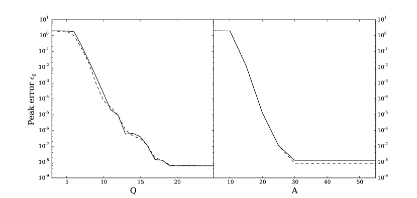
Figure 2: Convergence of the peak error $\epsilon_{0}$. Left: as function of discretization order $Q$ in the inner domain keeping $A=A_{0}$ fixed, right: as a function of absorption order $A$, keeping $Q\equiv Q_{0}$ fixed. Solid lines: FEM, dashed FEM-DVR. System parameters as in 1.

Fig. 2 shows thee discretization errors in the inner domain and complex scaled domain independently. Computations are with $Q,A_{0}$ varying $Q$ for the inner domain and $Q_{0},A$ varying $A$ for absorption. The joint parameters $Q_{0},A_{0}$ are chosen such that the solution is maximally accurate. As expected, errors drop exponentially with $Q$, and also absorption improves exponentially beyond a minimum number of $A\gtrsim 12$.

III.4 Discussion and conclusions on FEM-DVR

The simple conclusion of this first part is that FEM-DVR is completely at par with FEM, at least as far as perfect absorption is concerned. Considering the great simplification for the computation of integrals and, more importantly, the gains in operations count, ease of implementation, and ease of parallelization it is certainly to be preferred over a full blown FEM method. There is only a single point where we see some advantage of computing the integrals exactly: FEM eigenvalue estimates are variational upper bounds, while FEM-DVR approximations may drop below the true value. The actual errors are, according to our observation, of similar magnitude in both methods. In practice, the upper bounding property will rarely be of great importance.

Figure 3: Local error $\epsilon(x)$ for absorption in a finite box as the box $[-X_{\rm max},X_{\rm max}]$ is extended by adding elements in the absorbing domain. Size of all elements is $x_{n}-x_{n-1}=5$ and order is fixed at $Q=A=21$.

Our conclusion is at variance with previous reports on absorption using FEM-DVR. In Ref. Tao et al. (2009) the infinite range idea was not used. However, at some expense as to efficiency, also a standard DVR discretization using only polynomials without exponential damping produces highly accurate results. This was reported for FEM in Scrinzi (2010) and can be reconfirmed for FEM-DVR here. Fig. 3 shows the errors $\epsilon(x)$ of a discretization where the infinite intervals were replaced by an increasing number of finite elements of the constant order $Q_{0}$. One sees that errors can be very well controlled and no artifacts appear also in the area $|x|\sim R_{0}$. In spite of similar discretization sizes, the calculations in Tao et al. (2009) were reported to be instable, especially near $|x|=R_{0}$.

IV Generalized FD schemes

In FD schemes there is usually no explicit reference made to an underlying basis, but rather one is contented with representing the wavefunction at the grid points. In reality also FD uses a hypothesis for evaluating the derivatives: in standard applications one assumes that in the vicinity of a grid point $x_{j}$ the solution can be well approximated by a linear combination of polynomials $f^{(j)}_{k}(x)$. We first re-derive the standard schemes in analogy to the discussion of the FEM method above and then generalize the approach for non-differentiable solutions.

Standard symmetric FD schemes on equidistant one-dimensional grids $x_{j}=x_{0}+jh,j=0,\ldots,J$ are obtained by assuming that in the vicinity of each point $x_{j}$ one can write

$$\Psi(x)\approx\sum_{k=-P}^{P}f^{(j)}_{k}(x)c_{k}.$$ (30)

The “interpolation hypothesis” is that the functions $f^{(j)}_{k}$ are polynomials. We treat here only the case of symmetric schemes with an odd number of $Q=2P+1$ points and use the notation ${\widehat{F}}^{(j)}_{kl}:=f^{(j)}_{k}(x_{j+l})$ with the index ranges $l,k\in\{-P,\ldots,P\}$. The coefficients $c_{k}$ can be obtained from the neighboring function values $\Psi_{j+l}:=\Psi(x_{j+l})$ as

$$c_{k}=\sum_{l=-P}^{P}\left[\left({\widehat{F}}^{(j)}\right)^{-1}\right]_{kl}\Psi_{j+l}.$$ (31)

One readily obtains an approximation to the derivative $(\partial_{x}\Psi)(x_{j})=:\Psi^{\prime}_{j}$ as

$$\Psi^{\prime}_{j}\approx\sum_{l,k}(\partial_{x}f^{(j)}_{k})(x_{j})\left[\left({\widehat{F}}^{(j)}\right)^{-1}\right]_{kl}\Psi_{j+l}=:\sum_{l=-P}^{P}d^{(j)}_{l}\Psi_{j+l}.$$ (32)

Arranging the pointwise finite difference rules $d^{(j)}_{l}$ into a matrix ${\widehat{D}}^{(1)}_{j,j+l}=d^{(j)}_{l}$ we find for the finite difference approximation of the first derivative

$$\vec{\Psi}^{\prime}={\widehat{D}}^{(1)}\vec{\Psi}.$$ (33)

The same construction principle can be used for higher derivatives or actually any operator composed of derivatives and multiplicative operators.

Eq. (32) is suitable for the construction of the schemes in numerical practice, if only one avoids ill-conditioning of ${\widehat{F}}^{(j)}$. Almost any choice for the $f^{(j)}_{k}$, e.g. orthogonal polynomials or Lagrange polynomials at well-separated support points, will suffice.

IV.1 Non-equidistant, discontinuous, and complex scaled schemes

A standard way of constructing FD schemes for non-equidistant grids is based on the very same coordinate scaling discussed in the preceding section. Let us assume that the non-equidistant grid is defined by some monotonically increasing function as

$$x_{j}=\Lambda(y_{j})\text{ with }y_{j}=0,h,2h,\ldots,$$ (34)

which transforms the representation on the non-equidistant $x_{j}$ grid into a representation on the equidistant $y_{j}$ grid. For example, for exponential sampling of $x\geq 0$ one can choose $\Lambda(y)=\exp(y)-1,j=0,\ldots,N-1$ or $y=\log(1+|x|)$. For deriving the necessary transformation of the operators and for constructing norm-conserving schemes, it is useful to adhere to the notation of section II and consider the coordinate transformation as a unitary transformation $\Psi\to\Psi_{a}=U_{a}\Psi$, Eq. (3).

The key to suitable FD schemes in the transformed coordinates is to realize that the interpolation hypothesis for the transformed solution in general must differ from the original one. Suppose a set of functions $f^{(j)}_{k}$ is in some sense an optimal interpolation hypothesis for the unstretched $\Psi(x)$ near the point $x_{j}$. Then the transformed functions

$$f^{(j)}_{a;k}(y):=(U_{a}f^{(j)}_{k})(y)$$ (35)

will be equally optimal for interpolating $\Psi_{a}(y)$ near the point $y_{j}=\Lambda^{-1}(x_{j})$.

Assume that the interpolation hypothesis $f^{(j)}_{k}(x)$ of the original problem are polynomials, i.e. the standard finite difference scheme of a given order. Then in almost all cases the equally optimal interpolation hypothesis $f^{(j)}_{a,k}(y)=\lambda(y)^{-1/2}f^{(j)}_{k}(\Lambda(y))$ for the transformed solution $\Psi_{a}(y)$ will not be polynomials and one needs to re-derive the corresponding finite difference scheme by Eq. (32).

In practice, the procedure for obtaining schemes for any transformed linear operator $B_{a}=U_{a}BU_{a}^{*}$ is very simple. Analogous to Eqs. (30) and (32) one writes

$$\Psi_{a}(y)=(U_{a}\Psi)(y)\approx\sum_{k=-P}^{P}(U_{a}f^{(j)}_{k})(y)c_{k}=\sum_{k=-P}^{P}\lambda(y)^{1/2}(f^{(j)}_{k}(\Lambda(y))c_{k}$$ (36)

$$(B_{a}\Psi_{a})(y_{j}) = (U_{a}BU_{a}^{*})\Psi_{a}(y_{j})\approx\sum_{k=-P}^{P}(U_{a}Bf^{(j)}_{k})(y)c_{k}$$ (37)

$$= \sum_{k=-P}^{P}\lambda(y_{j})^{1/2}(Bf^{(j)}_{k})(\Lambda(y_{j}))c_{k}.$$

With the notation $\left({\widehat{F}}^{(j)}_{a}\right)_{lk}=\lambda(y_{l})^{1/2}(f^{(j)}_{k}(\Lambda(y_{l}))$ one obtains the adjusted scheme at point $y_{j}$ as

$$b_{a;l}^{(j)}=\sum_{k=1}^{Q}\lambda(y_{j})^{1/2}(Bf^{(j)}_{k})(\Lambda(y_{j}))\left[\left({\widehat{F}}^{(j)}_{a}\right)^{-1}\right]_{kl}.$$ (38)

For the first derivative $[\partial_{y}]_{a}$ we insert $Bf^{(j)}_{k}=\left[f^{(j)}_{k}\right]^{\prime}$ into Eq. (38), for the second derivative $[\partial_{y}^{2}]_{a}$ we insert $Bf^{(j)}_{k}=\left[f^{(j)}_{k}\right]^{\prime\prime}$ etc. As long as all transformations $U_{a}$ are unitary, one obtains symmetric schemes for ${\vec{\Psi}}_{a}$, provided that the original problem gives symmetric schemes.

The adjustment of $f^{(j)}_{a,k}$ is particularly important, when the transformation $\Lambda$ is not analytical. This is for example the case, when we want to switch from constant spacing $\Delta x_{1}$ in one region to a different constant spacing $\Delta x_{2}$ in some other region, possibly with a smooth, say linear, transition in between. If we attempt to approximate the transformed solution $\Psi_{a}(y)$ by higher order polynomials in $y$, i.e. when we use standard higher order FD schemes, we will observe a loss of the convergence order. Assuming the original $\Psi(x)$ has a convergent Taylor expansion, the solution w.r.t. to the transformed coordinate $\lambda^{1/2}(y)\Psi_{a}(y)=\Psi(\Lambda(y))$ only has a continuous first derivative $\partial_{y}$. Already the second derivative will be discontinuous and all higher derivatives show $\delta$-function like singularities at the boundaries between constant and linearly changing spacing, which disqualifies any attempt of expanding into a convergent Taylor series. Making the transition smoother only postpones the problem to higher orders. On the other hand, we will demonstrate below that adjusting $f^{(j)}_{a,k}$ and using Eq. (38) for the operators preserves the approximation order and no extra computational cost ensues apart from the initial construction of the local schemes $b_{a;l}^{(j)}$.

From the discussion it is clear that we can also use transformations generated by non-differentiable $\lambda(x)$, as they arise in ECS. All we need to do is to replace polynomials of standard FD schemes with their transformed counterparts. Finally, also the idea underlying the irECS discretization discussed above can be transferred to FD schemes. Considering the approximately exponentially spaced Radau quadrature points appearing in the FEM-DVR implementation of irECS, we see that the essential point of irECS is that the function is sampled at rapidly increasing spacing rather than uniformly. By uniting complex scaling with non-equidistant sampling we will obtain nearly as efficient absorption scheme with FD as irECS with FEM-DVR discretization.

IV.2 Absorption with equidistant FD grids

We first investigate complex scaling with equidistant grids for the model Hamiltonian (22). We will show that comparable accuracies are reached for FEM-DVR and FD at equal grid sizes and equal orders $Q_{n}$.

We again use the transformation defined by Eq. (24) with $a=\exp(i/2)$ and $R_{0}=25$ and FD schemes are constructed according to Eq. (38). The same constant order $Q_{n}\equiv 21$ is used in FD and FEM-DVR calculations on 1200 grid points in a computational box $[-150,150]$. Fig. 4 compares complex scaled densities $|\Psi_{a}(x)|^{2}$ and errors of the two methods relative to a converged calculation on a large box without using absorbing boundaries. Comparing unscaled $|\Psi(x)|^{2}$ with complex scaled $|\Psi_{a}(x)|$ densities one can clearly discern the suppression of the density to below $10^{-15}$ as the solution approaches the box boundaries. On the level of densities FD and FEM-DVR results are indistinguishable. Also, relative to a fully converged unscaled calculation, errors in the inner region are comparable.

Figure 4: Densities of the unscaled $|\Psi(x)|^{2}$ (dot-dashed line) and the complex scaled $|\Psi_{a}(x)|^{2}$ system (solid line). Damping by complex scaling at large $|x|$ is clearly exposed. Inset: relative errors $\epsilon(x)$ in the inner domain for DVR and FD at equal grid sizes and order.

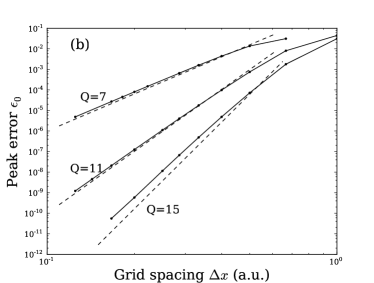
Figure 5: Convergence of peak relative error $\epsilon_{0}$ on the inner domain: (a) convergence with $Q$ for 1600 equidistant grid points on $[-200,200]$, (b) convergence with $\Delta x$, dashed lines $\Delta x^{Q-1}$. At $Q=15$ the actual convergence is only $\approx\Delta x^{13}$.

For completeness we show in Fig. 5 that the error drops exponentially with the FD order $Q$. This proves the full consistency and that the non-differentiable nature of the complex scaled solution is fully accounted for by the generalized FD scheme.

IV.3 Absorption with exponential FD grids

Having established standard ECS for FD grids, as a last step we implement the idea underlying irECS also for FD schemes. As discussed, this consists in exponentially sampling the scaled solution $\Psi_{a}$ in the absorbing domain. In the notation introduced above, exponential sampling can be achieved by applying a unitary transformation to the complex scaled solution $\Psi_{a}(y)$:

$$\Psi_{a}(y)\to\Psi_{a,\gamma}(z)=(W_{\gamma}\Psi_{a})(z),$$ (39)

where $W_{\gamma}$ is a real scaling transformation with

$$\lambda(z)=\left\{\begin{array}[]{ll}1&\text{ for }|z|<R_{0}\\ \exp[\gamma(|z|-R_{0})]&\text{ for }|z|\geq R_{0}\end{array}\right..$$ (40)

For the comparisons we use a fixed complex scaling radius $R_{0}=25$ and fixed complex scaling phase $a=\exp(i/2)$ as above. All complex scaled calculations are performed on the interval $[-100,100]$ with a total of 400 grid points. This allows accuracies of the density of $\lesssim 10^{-7}$ in unscaled domain $[-25,25]$, if absorption is perfect. Fig. 6 shows the complex scaled $|\Psi_{a}(y)|^{2}$ with equidistant grid and the complex scaled $|\Psi_{\gamma,a}(z)|$ with exponential grids in the scaled domain for $\gamma=0.1,0.2,0.35$. The spatial damping of the solution by the complex scaling transformation is clearly visible. Near the boundaries the equidistant grid solution $|\Psi_{a}|^{2}$ drops to $\sim 10^{-9}$. The effect of the Dirichlet boundary condition at $|y|=100$ is clearly visible, but has no consequences on the accuracy level of interest. The exponential grid maps the absorbing domain into smaller boundary layers outside $[-25,25]$. An optimum is reached near $\gamma=0.2$: the density drops to below the level $\lesssim 10^{-9}$ for all $|z|>40$. Larger contraction to $\gamma=0.35$ does not lead to further gains: although the solution shrinks to smaller $|z|$ initially, the exponential spacing $x_{j}=x(z_{j})$ is becoming too wide to represent the solution in the asymptotic region. An artefact on the level $\sim 10^{-5}$ appears which causes reflection errors. As shown in the figure, the artefact can be fully suppressed by reducing the grid spacing, but this defeats the purpose of minimizing the number of points used for absorption.

Figure 6: The irECS method for FD schemes. Solid lines: equidistant grid $\gamma=0$ and exponential scaling in the absorbing region. Spacing of the transformed grid $\Delta z=0.25$ and order $Q=21$. At $\gamma=0.35$ insufficient sampling leads to artefacts. Dashed line: with spacing $\Delta z=0.125$ exponent $\gamma=0.125$ does not show artefacts.

Finally, we investigate the dependence of absorption on $\gamma$ and $\theta$ for FD and FEM-DVR. In both methods we use the same number of 201 discretization points in the unscaled domain $[-25,25]$ and the same order $Q=21$, i.e. a 21 point scheme for FD and degree 20 polynomials for FEM-DVR, and we use the same number of $A=60$ points for absorption. At the grid spacing of $\Delta z=0.25$ this amount to Dirichlet boundary conditions at $|z|=40$ for FD. Note that this results in matrices the same size and of comparable sparsity in the inner region, with band-width 21 for FD and near block-diagonal matrices of blocks $21\times 21$ for FEM-DVR. Fig. 7 shows the relative errors of $|\Psi(x)|^{2}$ in the inner domain as obtained with either method. In FD the range of admissible $\gamma$ remains smaller than in FEM-DVR: as large $\gamma$ lead to a stronger contraction of the wave function, we see that the profit from the irECS idea is somewhat lower in FD.

Figure 7: Relative error of FEM-DVR (left) and FD (right) schemes as a function of exponent $\gamma$ and scaling angle $\theta$ at equal number of discretization points and comparable matrix sparsity. The admissible $\gamma$-range is narrower for FD, $\theta$ can be chosen in a wide range with either method.

IV.4 Smooth exterior scaling

We have demonstrated that the generalized FD schemes as well as FEM-DVR grids allow for discontinuous scaling functions $\lambda(x)$. A fortiori we expect smooth exterior scaling to work correctly, if implemented by the above principles. This is indeed the case. We use the scaling function

$$\lambda(y)=\left\{\begin{array}[]{ll}1&\text{ for }|y|<R_{0}\\ 1+(a-1)s(|y|)&\text{ for }R_{0}<|y|<R_{1}\\ a&\text{ for }|y|>R_{1},\end{array}\right.$$ (41)

where the $3^{rd}$ order polynomial $s(y)$ smoothly connects the inner domain with the region $|y|>R_{1}$ such that $\lambda(y)$ is differentiable at $y=R_{0}$ and $y=R_{1}$. Applying the same procedure as above and using $R_{1}=45$, i.e. smoothing over a range of $20\,au$, we find essentially identical results as for the abrupt transition used earlier, see Fig. 8.

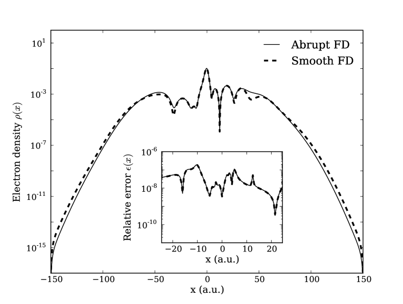
Figure 8: Abrupt (solid line) vs. smooth ECS (dashed line). Exponential suppression is slightly less with smooth scaling, errors in the unscaled region are identical.

The usual motivation for smooth scaling is not to use the generalized schemes but to apply standard schemes. There is no unique way for defining such a scheme for a polynomial interpolation hypothesis. There are two different possibilities: one by bringing the scaled second derivative Eq. (7) to a form that allows the use of standard FD schemes for $\partial_{y}$ and $\partial_{y}^{2}$ without increase of band-width

$$[\partial_{x}^{2}]_{a}=U_{a}\partial_{x}^{2}U_{a}^{*}=\frac{1}{\lambda}\partial_{y}^{2}\frac{1}{\lambda}-\frac{1}{2}\frac{\lambda^{\prime}}{\lambda^{2}}\partial_{y}\frac{1}{\lambda}+\frac{1}{\lambda}\partial_{y}\frac{1}{2}\frac{\lambda^{\prime}}{\lambda^{2}}-\frac{1}{4}\left(\frac{\lambda^{\prime}}{\lambda^{2}}\right)^{2}.$$ (42)

In a second approach, one can use the procedure for constructing finite difference schemes that lead to Eq. (32) for the complete operator (42) with polynomial interpolation in place of the correctly scaled polynomials. The latter fully uses the polynomial interpolation hypothesis, the former introduces some additional approximations in evaluating the transformed derivatives of the polynomials $[\partial_{x}^{2}]_{a}p_{k}(y)$. Note that in both cases the polynomial interpolation hypothesis is unjustified and the approximation cannot be successful beyond the lowest orders.

For the present demonstration we only study the second possibility, i.e. using the full, but incorrect polynomial interpolation without making further approximations. The limitation of convergence order for the polynomial interpolation hypothesis applied to a smoothly exterior scaled grid is illustrated in Fig. 9. For orders Q=3 and Q=5 polynomial and scaled interpolation give essentially the same result. However, while the correctly scaled interpolations shows steady exponential convergence at $Q=7,9$, no further gains can be made by increasing the order with the unscaled polynomial hypothesis. For higher accuracies one is forced to increase the of number grid points, which causes exceeding numerical cost not only in terms of the problem size but also in stiffness of the equations.

Figure 9: Convergence with order $Q$ for scaled and standard polynomial schemes. Smooth exterior scaling with a third degree polynomial smoothing function on an equidistant grid were used. Relative errors $\epsilon(x)$ in the unscaled region $[-25,25]$ are show for $Q=3,5,7,9$. Scaled schemes errors decrease exponentially with $Q$ (dashed lines). For polynomial schemes (solid lines) no gain is made for $Q>7$ ). Calculations are with $600$ points on the interval $[-80,80]$. The thick solid line is for a standard polynomial scheme with $Q=7$ and as many as 4800 points on $[-80,80]$.

Without demonstration, we only remark that also for the FEM-DVR scheme smooth transition does not bear any advantage over the abrupt transition used in the FEM-DVR calculations above. On the contrary, the rather complicated smoothly scaled operators must be programmed and the finite modulation of the solution in the transition region usually requires more grid points there, which in turn may raise the stiffness of the dynamical equations.

V Conclusions

With the present studies we have demonstrated that grid methods allow for highly efficient absorption schemes. The irECS method had been originally developed using a finite element implementation, where also the far superior performance of irECS compared to multiplicative CAPs and MFA had been highlighted. With the present extension of the method to FEM-DVR and FD grids one has discretizations that are easy to implement, have low floating counts, and are straight forward for parallelization. The latter point may be the most important advantage. While in transferring irECS to FEM-DVR no practical problems of any kind were encountered, we had to derive a new approach to FD for complex scaled problems. In fact, the computation of scaled schemes is technically simple and provides schemes that are as nearly as efficient in terms of discretization size as the FEM and FEM-DVR schemes of the same order. In particular, they can be pushed to high orders with exponential reduction of errors to near machine precision.

We have shown that irECS can be considered as ECS with an exponential grid in the absorbing domain. Both, in FEM-DVR and in FD the transition from the equidistant unscaled to the exponentially spaced absorbing region is numerically seamless, i.e. it does not produce any artefacts compared to an equidistant grid. The numerical gain by the reduction of grid points is substantial and no increase in stiffness was observed.

We have further studied smooth exterior scaling and shown that one can smoothen the transition between scaled and unscaled region. This case was only discussed for the FD implementation, as one usually resorts to such a procedure to circumvent manifest problem that arises for using standard FD schemes across abrupt transitions. Absorption works for smooth scaling as well as it does for abrupt scaling, but only if scaled, non-polynomial schemes are used. With standard polynomial schemes, lack of differentiability leads to a strict limitation of the consistency to the point where the corresponding higher derivatives of the smoothing function become singular. Smoothing does not bear any mathematical or computational advantage as compared to abrupt transitions, on the contrary, it tends to complicate implementation as the essentially arbitrary smoothing transformation must be incorporated into the scheme. Therefore, at least from the present work, we would advice to use abrupt changeovers wherever possible.

The FD schemes for non-equidistant grids, in particular the abrupt and reflectionless transition between grid spacings occurring in abrupt exterior scaling, may be of broad interest for uses beyond the problem of absorbing boundaries considered here. Locally adapted FD grids are frequently used in literature. To the best of our knowledge, the approach presented here and proven to fully maintain convergence orders is novel. In future work, we plan to investigate the problem for non-equidistant grid representations of Maxwell’s equations.

References

- McCurdy et al. (1991) C. W. McCurdy, C. K. Stroud, and M. K. Wisinski, Phys. Rev. A 43, 5980 (1991).
- Scrinzi (2010) A. Scrinzi, Phys. Rev. A 81, 053845 (2010).
- Scrinzi et al. (2014) A. Scrinzi, H. P. Stimming, and N. J. Mauser, J. Comput. Physics pp. 98–107 (2014).
- Telnov et al. (2013) D. A. Telnov, K. E. Sosnova, E. Rozenbaum, and S.-I. Chu, Phys. Rev. A 87, 053406 (2013), URL http://link.aps.org/doi/10.1103/PhysRevA.87.053406.
- Dujardin et al. (2014) J. Dujardin, A. Saenz, and P. Schlagheck, Applied Physics B 117, 765 (2014), ISSN 0946-2171, URL http://dx.doi.org/10.1007/s00340-014-5804-3.
- De Giovannini et al. (2015) U. De Giovannini, A. Larsen, and A. Rubio, The European Physical Journal B 88, 56 (2015), ISSN 1434-6028, URL http://dx.doi.org/10.1140/epjb/e2015-50808-0.
- Miller et al. (2014) M. R. Miller, C. Hernández-García, A. Jarón-Becker, and A. Becker, Phys. Rev. A 90, 053409 (2014), URL http://link.aps.org/doi/10.1103/PhysRevA.90.053409.
- (8) A. Saenz, private communication.
- Rom et al. (1990) N. Rom, E. Engdahl, and N. Moiseyev, J. Chem. Phys. 93, 3413 (1990).
- (10) The tRecX Homepage, URL http://homepages.physik.uni-muenchen.de/~armin.scrinzi/tRecX.
- Reed and Simon (1982) M. Reed and B. Simon, Methods of Modern Mathematical Physics (Academic, New York, 1982), p. 183ff.
- Manolopoulos and Wyatt (1988) D. Manolopoulos and R. Wyatt, Chemical Physics Letters 152, 23 (1988), ISSN 0009-2614, URL http://www.sciencedirect.com/science/article/pii/0009261488873226.
- Scrinzi and Elander (1993) A. Scrinzi and N. Elander, J. Chem. Phys. 98, 3866 (1993).
- Hofmann et al. (2014) C. Hofmann, A. S. Landsman, A. Zielinski, C. Cirelli, T. Zimmermann, A. Scrinzi, and U. Keller, Phys. Rev. A 90 (2014), ISSN 1050-2947.
- Majety et al. (2015) V. P. Majety, A. Zielinski, and A. Scrinzi, New. J. Phys. 17 (2015), ISSN 1367-2630.
- Majety and Scrinzi (2015) V. P. Majety and A. Scrinzi, Phys. Rev. Lett. 115, 103002 (2015), URL http://link.aps.org/doi/10.1103/PhysRevLett.115.103002.
- Zielinski et al. (2014) A. Zielinski, V. P. Majety, S. Nagele, R. Pazourek, J. Burgdörfer, and A. Scrinzi, arXiv:1405.4279 [physics.atom-ph] (2014).
- Torlina et al. (2015) L. Torlina, F. Morales, J. Kaushal, I. Ivanov, A. Kheifets, A. Zielinski, A. Scrinzi, H. Muller, S. Sukiasyan, M. Ivanov, et al., Nature Physics 11, 503 (2015).
- Tao et al. (2009) L. Tao, W. Vanroose, B. Reps, T. N. Rescigno, and C. W. McCurdy, Phys. Rev. A 80, 063419 (2009).
- Zielinski et al. (2015) A. Zielinski, V. P. Majety, and A. Scrinzi, (in preparation) (2015).
- Combes et al. (1987) J. Combes, P. Duclos, M. Klein, and R. Seiler, Communications in Mathematical Physics 110, 215 (1987), ISSN 0010-3616, URL http://dx.doi.org/10.1007/BF01207364.