A family of periodic solutions of the three body problem. Light version

Abstract.

In this paper we describe a 1-dimensional family of initial conditions $\Sigma$ that provides reduced periodic solution of the three body problem. This family $\Sigma$ contains a bifurcation point and extend the periodic solution described in [7]. This 1-dimensional family is the union of two embedded smooth curves. We will explain how the trajectories of the bodies in the solutions coming from one of the embedded curves have two symmetries while those coming from the other embedded curve only have one symmetry. The Round Taylor Method is a numerical method implemented by the author to keep track of the global error and the round-off error. A second version of this paper, same title with the “light version” part removed, will include analysis of the error of the solutions using the Round Taylor Method.

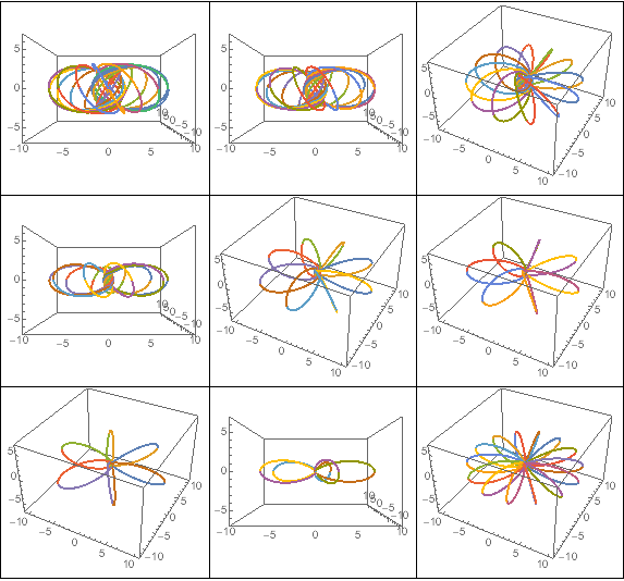
Figure 1. Trajectory of one of the bodies for some of the periodic solutions described in this paper

1. Introduction

In [7] the author considered the family of solutions of the three body problem described by the parameters $a$ and $b$ suggested by the following figure.

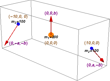
Figure 2. A family of solutions of the three body problem described by the parameters $a$ and $b$.

Three functions $F(t,a,b)$, $R(t,a,b)$ and $\Theta(t,a,b)$ describe the solution of the three body problem with initial conditions described in Figure 2, more precisely we have that

$$x(t) = (0,0,F(t,a,b))$$

$$y(t) = (R(t,a,b)\cos(\Theta(t,a,b)),R(t,a,b)\sin(\Theta(t,a,b)),-F(t,a,b))$$

$$z(t) = (-R(t,a,b)\cos(\Theta(t,a,b)),-R(t,a,b)\sin(\Theta(t,a,b)),-F(t,a,b))\,,$$

satisfy the three body problem equations, provided that the following ODE system holds true

(1.1) $$\ddot{F}=-\frac{400}{S^{3}}F,\,\quad\ddot{R}=\frac{100a^{2}}{R^{3}}-\frac{25}{R^{2}}-\frac{200R}{S^{3}},\,\quad R^{2}\dot{\Theta}=10a,$$

with $\,R(0,a,b)=10,\,F(0,a,b)=0,\,\Theta(0,a,b)=0$, where $S=\sqrt{R^{2}+4F^{2}}$

where $\dot{G}$ denotes the partial derivative with respect to $t$ for any function $G(t,a,b)$. We are assuming that the gravitational constant is 1. We will be referring to the solution of the three body problem described by the differential equation (1) as $\phi(a,b)$.

where $\dot{G}$ denotes the partial derivative with respect to $t$ for any function $G(t,a,b)$. We are assuming that the gravitational constant is 1. We will be referring to the solution of the three body problem described by the differential equation (1) as $\phi(a,b)$.

It is not difficult to show that anytime we find a point $(T,a,b)$ such that $\dot{F}(T,a,b)=\dot{R}(T,a,b)=0$, then the solution $\phi(a,b)$ is reduced periodic with period $4T$. We will call these solutions odd/even solutions because from the point of view of $t=0$ the function $F$ is an odd function with respect to $t$, but from the point of view of $t=T$, both functions $F$ and $R$ are even. Also, it is not difficult to show that anytime we find a point $(T,a,b)$ such that $F(T,a,b)=\dot{R}(T,a,b)=0$, then the solution $\phi(a,b)$ is reduced periodic with period $2T$. We will call these solutions odd solutions because from the point of view of $t=0$ the function $F$ is an odd function. We point out that every odd/even function is also odd due to the fact that if $\dot{F}(T,a,b)=\dot{R}(T,a,b)=0$, then $F(2T,a,b)=\dot{R}(2T,a,b)=0$.

In [7] the author proved the existence of a small path $\alpha\subset R^{3}=\{(T,a,b):T,a,b\in R\}$ of odd/even solutions. In this paper we extend this path to a path $S_{1}$ of odd/even solutions: the embedded curve $P_{3}BP_{2}$ in Figure 3. This path starts near a periodic solution where the body in the center remains motionless and the other two bodies move along an ellipse ($b$ near $0$). The path ends near a motion with a double coalition (in this case $a$ is near 0). We also provide a path $S_{2}\subset R^{3}$ of odd solutions: the embedded curve that contains the curve $P_{1}B$ in Figure 3. This path $S_{2}$ starts near a motion with a triple collision (in this case $a$ is near 0). This path $S_{2}$ intercepts the path $S_{1}$ in a single point that can be thought as a bifurcation point of the set of reduced periodic solutions. The author is not sure if this path will continue to be an unbounded curve.

A second version of this paper will use the Round Taylor Method [7] to compute the error and show that the difference between the initial conditions and the values of the solution after a period $T$ is small.

2. Graph of the path of initial conditions that provides reduced periodic solutions.

This section describes a path $\subset R^{3}=\{(T,a,b):T,a,b\in R\}$ with the property that for any $(T,a,b)$ in $S$, the solution $\phi(a,b)$ is reduced periodic with period $T$, this is, the relative position of the three bodies in the solution $\phi(a,b)$ repeats every $T$ units of time. Figure 3 is an image of the path $S$.

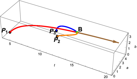
Figure 3. $P_{1}$ has coordinates $(5.0063\dots,0.109392\dots,1.16473\dots)$, which means that when $a=0.109392\dots$, and $b=1.16473\dots$, then, the solution $\phi(a,b)$ has period $T=5.0063\dots$. The other coordinates are: $P_{2}=(12.7012\dots,0.0437163\dots,3.19541\dots)$, $P_{3}=(9.9472\dots,4.73605\dots,0.2)$ and, the coordinate for bifurcation point are $B=(14.6072\dots,2.08181\dots,3.19493\dots)$.

Recall that the distances between the three bodies depend exclusively only on the functions $R(t)$ and $F(t)$. More precisely, the distance between the two bodies that go around the $z$ axis is $2R(t)$ and the distance between the body that moves on the $z$-axis and any of the other two bodies is given by $\sqrt{R(t)^{2}+F(t)^{2}}$.

2.1. The solution given by the point $P_{3}=(9.9472\dots,4.73605\dots,0.2)$

This solution is very close to the solution when the body in the center stays still and the other two bodies move on a perfect circle. Figure 4 shows the graphs of the functions $F$ and $R$ associated with this solution. We can see how the body in the center given by $(0,0,F(t))$ moves very little and the other two bodies given by $(R(t)\cos(\Theta(t)),R(t)\sin(\Theta(t)),-F(t))$ and $(-R(t)\cos(\Theta(t)),-R(t)\sin(\Theta(t)),-F(t))$ stay near the circle of radius 10 on the $x$-$y$ plane with center at the origin.

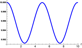
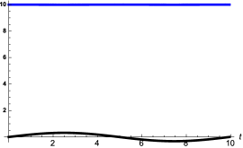
Figure 4. For the point $P_{3}$, the image on the left shows the graph of the function $F$, the image on the center shows the graph of the function $R$ and the image on the right shows both functions.

2.2. The solution given by the point $P_{2}=(12.7012\dots,0.0437163\dots,3.19541\dots)$

For this motion the body in the center oscillates from $(0,0,-6.01695\dots)$ to $(0,0,6.01695\dots)$. This solution is very close to a solution with a double collision. Figure 5 shows the graphs of the functions $F$ and $R$ associated with this solution. We can see how after a quarter of a period the two bodies that go around the $z$-axis are very close to each other ($R$ is very small, it is near $0.0547972$) at this instance the body in the center is at its highest point while the other two bodies are both very close to the point $(0,0,-6.01695\dots)$.

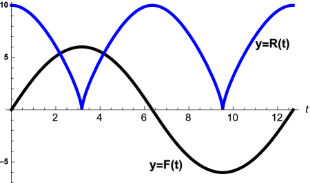
Figure 5. The functions $F$ and $R$ associated with the reduced periodic solution given by the point $P_{2}$.

2.3. The solution given by the point $P_{1}=(5.0063\dots,0.109392\dots,1.16473\dots)$

For this motion the body in the center oscillates from $(0,0,-1.52497\dots)$ to $(0,0,1.52497\dots)$. This solution is very close to a solution with a triple collision. Figure 6 shows the graphs of the functions $F$ and $R$ associated with this solution. We can see how after half of a period the three bodies are very close to the origin. $F$ is zero and $R$ is very small, it is near $0.0369262$.

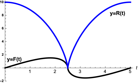
Figure 6. The functions $F$ and $R$ associated with the reduced periodic solution given by the point $P_{1}$.

2.4. The solution given by the point $B=(14.6072\dots,2.08181\dots,3.19493\dots)$

This is the bifurcation point of the path of solutions. Figure 7 shows the graphs of the functions $F$ and $R$ associated with this solution.

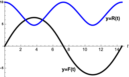
Figure 7. The functions $F$ and $R$ associated with the reduced periodic solution given by the point $B$

Let us call $S_{1}$, the part of the path contained in $S$ given by the smooth curve that connects $P_{2}$, $B$ and $P_{3}$, see Figure 3. Likewise, let us call $S_{2}$, the part of the path contained in $S$ given by the smooth curve that connects $P_{1}$, $B$ and also contains the part of $S$ that has an arrow at the end. All the points in the path $S_{1}$ are odd/even solutions; all of them share the symmetry given by the functions shown in Figure 7. More precisely: With respect to the origin, the function $F$ is odd and the function $R$ is even and with respect to $t=\frac{T}{4}$, both functions $F$ and $R$ are even. The solutions associated with points in the curve $S_{2}$ different from the point $B$ do not share these two symmetries. With respect to $t=0$, the function $F$ is odd and the function $R$ is even. There is not symmetry with respect to $t=\frac{T}{4}$. Figure 8 shows the function $F$ and $R$ for the solution associated with two points on $S_{2}$.

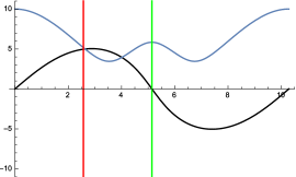
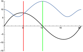
Figure 8. The image on the left shows the functions $F$ and $R$ associated with a point on the curve $S_{2}$ between $P_{1}$ and $B$. The image on the right shows these two functions for a point on the curve $S_{2}$ located after the point $B$. We can see how the symmetry with respect to the vertical line $t=\frac{T}{2}$ that is present for solutions coming from points in $S_{1}$ is not present in these solutions.

3. Procedure to obtain the points on the curve $S$ and the bifurcation point

3.1. Original ODE

The functions $F(t,a,b)$, $R(t,a,b)$ and $\Theta(t,a,b)$ satisfy the following ODE

$$\dot{x}_{1} = x_{3}$$

$$\dot{x}_{2} = x_{4}$$

$$\dot{x}_{3} = -\frac{400x_{1}}{\left(4x_{1}^{2}+x_{2}^{2}\right){}^{3/2}}$$

$$\dot{x}_{4} = \frac{100a^{2}}{x_{2}^{3}}-\frac{25}{x_{2}^{2}}-\frac{200x_{2}}{\left(4x_{1}^{2}+x_{2}^{2}\right){}^{3/2}}$$

$$\dot{x}_{5} = \frac{10a}{x_{2}^{2}}$$

with initial conditions

$$x_{1}(0)=0\quad x_{2}(0)=10\quad x_{3}(0)=b\quad x_{4}(0)=0\quad x_{5}(0)=0$$

This ODE will be referred to as the original ODE. We have that $x_{1}(t)$ provides $F(t,a,b)$, $x_{2}(t)$ provides $R(t,a,b)$, $x_{3}(t)$ provides $\dot{F}(t,a,b)$, $x_{4}(t)$ provides $\dot{R}(t,a,b)$ and $x_{5}(t)$ provides $\Theta(t,a,b)$

3.2. Extended ODE

The partial derivative of the functions $F(t,a,b)$, $R(t,a,b)$ and $\Theta(t,a,b)$ satisfy the following ODE

$$\dot{x}_{1} = x_{3}$$

$$\dot{x}_{2} = x_{4}$$

$$\dot{x}_{3} = -\frac{400x_{1}}{\left(4x_{1}{}^{2}+x_{2}{}^{2}\right){}^{3/2}}$$

$$\dot{x}_{4} = -\frac{200x_{2}}{\left(4x_{1}{}^{2}+x_{2}{}^{2}\right){}^{3/2}}-\frac{25}{x_{2}{}^{2}}+\frac{100a^{2}}{x_{2}{}^{3}}$$

$$\dot{x}_{5} = \frac{10a}{x_{2}{}^{2}}$$

$$\dot{x}_{6} = x_{8}$$

$$\dot{x}_{7} = x_{9}$$

$$\dot{x}_{8} = \frac{3200x_{6}x_{1}{}^{2}}{\left(4x_{1}{}^{2}+x_{2}{}^{2}\right){}^{5/2}}+\frac{1200x_{2}x_{7}x_{1}}{\left(4x_{1}{}^{2}+x_{2}{}^{2}\right){}^{5/2}}-\frac{400x_{2}{}^{2}x_{6}}{\left(4x_{1}{}^{2}+x_{2}{}^{2}\right){}^{5/2}}$$

$$\dot{x}_{9} = -\frac{300a^{2}x_{7}}{x_{2}{}^{4}}+\frac{200a}{x_{2}{}^{3}}+\frac{2400x_{1}x_{2}x_{6}}{\left(4x_{1}{}^{2}+x_{2}{}^{2}\right){}^{5/2}}+\frac{50x_{7}}{x_{2}{}^{3}}+\frac{600x_{2}{}^{2}x_{7}}{\left(4x_{1}{}^{2}+x_{2}{}^{2}\right){}^{5/2}}-\frac{200x_{7}}{\left(4x_{1}{}^{2}+x_{2}{}^{2}\right){}^{3/2}}$$

$$\dot{x}_{10} = \frac{10}{x_{2}{}^{2}}-\frac{20ax_{7}}{x_{2}{}^{3}}$$

$$\dot{x}_{11} = x_{13}$$

$$\dot{x}_{12} = x_{14}$$

$$\dot{x}_{13} = \frac{3200x_{11}x_{1}{}^{2}}{\left(4x_{1}{}^{2}+x_{2}{}^{2}\right){}^{5/2}}+\frac{1200x_{2}x_{12}x_{1}}{\left(4x_{1}{}^{2}+x_{2}{}^{2}\right){}^{5/2}}-\frac{400x_{2}{}^{2}x_{11}}{\left(4x_{1}{}^{2}+x_{2}{}^{2}\right){}^{5/2}}$$

$$\dot{x}_{14} = -\frac{300a^{2}x_{12}}{x_{2}{}^{4}}+\frac{2400x_{1}x_{2}x_{11}}{\left(4x_{1}{}^{2}+x_{2}{}^{2}\right){}^{5/2}}+\frac{50x_{12}}{x_{2}{}^{3}}+\frac{600x_{2}{}^{2}x_{12}}{\left(4x_{1}{}^{2}+x_{2}{}^{2}\right){}^{5/2}}-\frac{200x_{12}}{\left(4x_{1}{}^{2}+x_{2}{}^{2}\right){}^{3/2}}$$

$$\dot{x}_{15} = -\frac{20ax_{12}}{x_{2}{}^{3}}$$

with initial conditions

$$x_{1}(0) = 0$$

$$x_{2}(0) = 10$$

$$x_{3}(0) = b$$

$$x_{4}(0) = 0$$

$$x_{5}(0) = 0$$

$$x_{6}(0) = 0$$

$$x_{7}(0) = 0$$

$$x_{8}(0) = 0$$

$$x_{9}(0) = 0$$

$$x_{10}(0) = 0$$

$$x_{11}(0) = 0$$

$$x_{12}(0) = 0$$

$$x_{13}(0) = 1$$

$$x_{14}(0) = 0$$

$$x_{15}(0) = 0$$

This ODE will be referred to as the extendded ODE. We have that $x_{1}(t)$ provides $F(t,a,b)$, $x_{2}(t)$ provides $R(t,a,b)$, $x_{3}(t)$ provides $\dot{F}(t,a,b)$, $x_{4}(t)$ provides $\dot{R}(t,a,b)$, $x_{5}(t)$ provides $\Theta(t,a,b)$, $x_{6}(t)$ provides $\frac{\partial F}{\partial a}(t,a,b)$, $x_{7}(t)$ provides $\frac{\partial R}{\partial a}(t,a,b)$, $x_{8}(t)$ provides $\frac{\partial^{2}F}{\partial a\partial t}(t,a,b)$, $x_{9}(t)$ provides $\frac{\partial^{2}R}{\partial a\partial t}(t,a,b)$, $x_{10}(t)$ provides $\frac{\partial\Theta}{\partial a}(t,a,b)$, $x_{11}(t)$ provides $\frac{\partial F}{\partial b}(t,a,b)$, $x_{12}(t)$ provides $\frac{\partial R}{\partial b}(t,a,b)$, $x_{13}(t)$ provides $\frac{\partial^{2}F}{\partial b\partial t}(t,a,b)$, $x_{14}(t)$ provides $\frac{\partial^{2}R}{\partial b\partial t}(t,a,b)$ and $x_{15}(t)$ provides $\frac{\partial\Theta}{\partial b}(t,a,b)$.

These equations easily follows as an application of the chain rule. To exemplify this procedure let us compute $\dot{x}_{8}(t)$,

$$\dot{x}_{8} = \ddot{x}_{1}{}_{a}=\left(-400x_{1}\,\left(4x_{1}{}^{2}+x_{2}{}^{2}\right){}^{-3/2}\ \right)_{a}$$

$$= -400x_{6}\,\left(4x_{1}{}^{2}+x_{2}{}^{2}\right){}^{-3/2}+1200x_{1}\left(4x_{1}{}^{2}+x_{2}{}^{2}\right){}^{-5/2}\,\left(4x_{1}x_{6}+x_{2}x_{7}\right)$$

$$= \frac{3200x_{6}x_{1}{}^{2}}{\left(4x_{1}{}^{2}+x_{2}{}^{2}\right){}^{5/2}}+\frac{1200x_{2}x_{7}x_{1}}{\left(4x_{1}{}^{2}+x_{2}{}^{2}\right){}^{5/2}}-\frac{400x_{2}{}^{2}x_{6}}{\left(4x_{1}{}^{2}+x_{2}{}^{2}\right){}^{5/2}}$$

3.3. Getting the points on $S_{1}$

Ideally we want each point $(t,a,b)\in S_{1}$ to satisfy the system of equations $\{\dot{F}(\frac{t}{4},a,b)=\dot{R}(\frac{t}{4},a,b)=0\}$. From the paper [7] we know that there exist a point $\bar{P}_{0}=(\bar{t},\bar{a},\bar{b})$ near

$$P_{0}=(t_{0},a_{0},b_{0})=\left(\frac{13366894627923}{5000000000000},\frac{43170475352787}{10000000000000},\frac{1490359743}{1000000000}\right)$$

such that $\dot{F}(\bar{P}_{0})=\dot{R}(\bar{P}_{0})=0$. If we assume for a moment that we completely know the functions $F$ and $R$ in the whole ${R}^{3}$, then the way to find the curve $S_{1}$ would be simply, first, find the vector field $X=v_{1}\times v_{2}$, where $v_{1}=\nabla\dot{F}=(\ddot{F},\dot{F}_{a},\dot{F}_{b})$ and $v_{2}=\nabla\dot{R}=(\ddot{R},\dot{R}_{a},\dot{R}_{b})$ and second, find the integral curve of the vector field $X$ that goes through $\bar{P}_{0}$. Recall that the first entry of points in $S_{1}$ is 4 times the first entry of points in this integral curve. Notice that using the notation from section 3.2 we have that

$$\nabla\dot{F}=\left(-\frac{400x_{1}(t)}{\left(4x_{1}(t){}^{2}+x_{2}(t){}^{2}\right){}^{3/2}},x_{8},x_{13}\right)$$

and

$$\nabla\dot{R}=\left(\frac{25\left(-\frac{8x_{2}(t){}^{4}}{\left(4x_{1}(t){}^{2}+x_{2}(t){}^{2}\right){}^{3/2}}-x_{2}(t)+4a^{2}\right)}{x_{2}(t){}^{3}},x_{9},x_{14}\right)$$

Even though we do not know the vector field $\nabla\dot{F}$ and $\nabla\dot{R}$ everywhere, we can still use the idea of integrating the vector field $X$ using the Euler method. The next subsection explains the algorithm that we are using in this paper to get the points in $S_{1}$.

3.3.1. Continuation algorithm

For the Algorithm we select three small numbers $\epsilon_{1}$ and $\epsilon_{2}$ and $\epsilon_{3}$ that we use as tolerance for the error. We want $0<\epsilon_{1}<\epsilon_{2}$. Recall that we want to find solutions of the system $\{\dot{F}=\dot{R}=0\}$. We will be collecting the solution of this system of equations in a set called $TS$. To start with, we make, $TS=\{P_{0}\}$, the set which only element is the numerical solution that we know. We will use $P_{0}$ to start the algorithm.

1. Consider a point $Q_{0}=(\tilde{t},\tilde{a},\tilde{b})$ such that $|\dot{F}(Q_{0})|<\epsilon_{1}$ and $|\dot{R}(Q_{0})|<\epsilon_{1}$.

2. Make $Y=Q_{0}$ and select a positive real number $h$ and a positive integer $k$.

3. For $i=1$ to $i=k$ Do

   • Find the values of $X$ by numerically solving the extended ode (see section 3.2) using the values of $t$, $a$ and $b$ given by the entries of $Y$. This is, we integrate for $t$ units of time where $t$ is the first entry of $Y$ and we use the values of $a$ and $b$ given by the second and third entry of $Y$ to provide the initial conditions of the ode.

   • Make $Y=Y+\frac{h}{|X|}\,X$ and $q_{i}=Y$.

4. If for all $i=1\dots k$, $|\dot{F}(q_{i})|<\epsilon_{2}$ and $|\dot{R}(q_{i})|<\epsilon_{2}$ then go to the next numeral, otherwise go back to numeral (2) and select a smaller $h$ and/or a smaller $k$.

5. Find $Q_{1}$ such that $|\dot{F}(Q_{1})|<\epsilon_{1}$ and $|\dot{R}(Q_{1})|<\epsilon_{1}$ and such that it is near $q_{k}$ in the sense that $|q_{k}-Q_{1}|<\epsilon_{3}$

6. Make $TS=TS\cup\{Q_{1}\}\cup\cup_{k=1}^{k}\{q_{i}\}$

7. Go back to numeral (1) to start the process over by making $Q_{0}=Q_{1}$.

Definition 3.1.

We will call pillar points all the points $Q_{i}$ in the previous algorithm.

In our case the algorithm stopped or became difficult to carry near the point $P_{3}$ and $P_{2}$ because the ode was approaching a singularity near $P_{2}$ (recall that $P_{2}$ is close to a collision) and on the other hand the vector field $X$ is close to the zero vector near $P_{3}$.

As an example of the method, if we start with $Q_{0}=P_{0}$ and we use $\epsilon_{1}=10^{-6}$, $\epsilon_{2}=\epsilon_{3}=0.00005$, $h=0.001$ and $k=200$, then,

$q_{200}=(2.7219062659312807,4.212655007080421,1.6538674269975053)$

and we can use $Q_{1}=(2.72191575576588,4.212633490447383,1.6538497779324066)$.

3.4. Getting the points on $S_{1}$

Ideally we want each point $(t,a,b)\in S_{2}$ to satisfy the system of equations $\{F(\frac{t}{2},a,b)=\dot{R}(\frac{t}{2},a,b)=0\}$. If we assume for a moment that we completely know the functions $F$ and $R$ in the whole ${R}^{3}$, then the way to find the curve $S_{2}$ would be simply, first, find the vector field $Z=w_{1}\times w_{2}$, where $w_{1}=\nabla F=(\dot{F},F_{a},F_{b})$ and $w_{2}=\nabla\dot{R}=(\ddot{R},\dot{R}_{a},\dot{R}_{b})$ and second, find the integral curve of the vector field $Z$. Recall that the first entry of points in $S_{2}$ is twice the first entry of points in this integral curve. Notice that using the notation from section 3.2 we have that $\nabla F=\left(x_{3},x_{6},x_{11}\right)$. The points in $S_{2}$ are found using the algorithm described in section 3.3.1.

3.5. Getting the bifurcation point.

Recall that the solutions associated with points on $S_{1}$ are called odd/even solutions and those associated with points in $S_{2}$ are called even solutions. Having in mind the symmetries of the solutions, it is not a surprise that for points on the integral curve $\gamma$ of the vector field $X$ that passes to the point $\bar{P}_{0}$, the vector field $Z$ is parallel to the vector field $X$. The bifurcation point occurs because along $\gamma$, there is a point where the vector field $Z$ vanishes. In order to numerically compute the bifurcation point, we take the minimum of the set $\{|Z(\frac{t}{2},a,b)|:(t,a,b)\in S_{1}\}$. This minimum occurs at the point $B=(14.607249047056753,2.081806260749908,3.194934273913219)\in S_{1}$.

4. Periodic Solutions

Recall that a reduced periodic solution $\phi(a,b)$ with period $T$ is periodic if $\frac{\Theta(T,a,b)}{\pi}$ is a rational number. It is not difficult to see the values of the function $\Theta$ on the points on the $S$. In this section we will be selecting some values for $\Theta$ along the path $S$ that provides periodic solutions.

4.1. Periodic solution displayed on Figure 1

Every entry of the matrix in Figure 1 (located at the begging of the paper) shows the trajectory of one of the three bodies that moves periodically solving the three-body problem. The following table provides the initial conditions of these 9 periodic solutions. The first entry $T$ represent the period of the reduced periodic solution. This is, the positions and velocities after $T$ units of time agree with the initial positions and velocities up to a rotation of $\theta$ radians. This rotation $\theta$ is given in the second column of the table. Every color in these images show the trajectory after $T$ units of time. These points are part of the path $S_{2}$. These periodic solutions only one symmetry. The periodic solution given by the last row in this table is very close to a triple collision.

Coordinates:    $(T,a,b)$	$\Theta(T,a,b)$	Image
		location
(7.464725167070125, 1.332130235206886, 2.39131806234605)	$\frac{14\pi}{9}$	(1,1)
(6.692611549615348, 1.1189865713077587, 2.178542324667063)	$\frac{11\pi}{7}$	(1,2)
(6.156645197408822, 0.9203809141218081, 1.9818897189116862)	$\frac{8\pi}{5}$	(1,3)
(5.758992220584509, 0.72863210825991, 1.791870916952545)	$\frac{13\pi}{8}$	(2,1)
(5.454531817007846, 0.5397530375918577, 1.6029431700479464)	$\frac{5\pi}{3}$	(2,2)
(5.32949878269853, 0.4457220498597047, 1.5077112808284203)	$\frac{12\pi}{7}$	(2,3)
(5.220379172126002, 0.35201283725645105, 1.411839280497764)	$\frac{7\pi}{4}$	(3,1)
(5.1264630045948305, 0.25902392732426605, 1.3159094056731593)	$\frac{16\pi}{9}$	(3,2)
(5.096931182326409, 0.22679159236240487, 1.2822928944673215)	$\frac{9\pi}{5}$	(3,3)

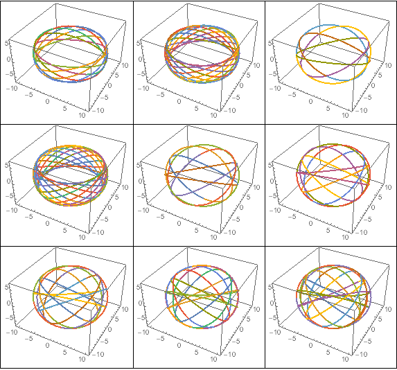
Figure 9. Trajectory of one of the bodies for some of the periodic solutions described in this paper.

4.2. Periodic solution displayed on Figure 9

Every entry of the matrix in Figure 9 (located at the end of the paper) shows the trajectory of one of the three bodies that moves periodically solving the three-body problem. The following table provides the initial conditions of these 9 periodic solutions. The first entry $T$ represent the period of the reduced periodic solution. This is, the positions and velocities after $T$ units of time agree with the initial positions and velocities up to a rotation of $\theta$ radians. This rotation $\theta$ is given in the second column of the table. Every color in these images show the trajectory after $T$ units of time. These points are part of the path $S_{1}$. These periodic solutions are odd/even solutions and therefore they have two symmetries.

Coordinates:    $(T,a,b)$	$\Theta(T,a,b)$	Image
		location
(10.694782129146047, 4.3162773916465715, 1.4916623030663265)	$\frac{17\pi}{8}$	(1,1)
(10.900907564917922, 4.205530359018152, 1.6642665366638942)	$\frac{15\pi}{7}$	(1,2)
(11.251546754899636, 4.020933846016405, 1.9098147447184282)	$\frac{13\pi}{6}$	(1,3)
(11.546587626864484, 3.8684643701482133, 2.0840362602898437)	$\frac{11\pi}{5}$	(2,1)
(12.005866456188725, 3.6348152391561275, 2.314439960284758)	$\frac{9\pi}{4}$	(2,2)
(12.482298481771874, 3.3941653076488447, 2.5161535540867117)	$\frac{16\pi}{7}$	(2,3)
(12.805950195048542, 3.229502929775678, 2.6373059506494907)	$\frac{7\pi}{3}$	(3,1)
(13.037980888481863, 3.10968118474065, 2.717938296845948)	$\frac{12\pi}{5}$	(3,2)
(13.211458502729283‘, 3.01851140163578‘, 2.775360523910528‘)	$\frac{17\pi}{7}$	(3,3)

4.3. Periodic solution displayed on Figure 10

Every entry of the matrix in Figure 10 (located at the end of the paper) shows the trajectory of one of the three bodies that moves periodically solving the three-body problem. The following table provides the initial conditions of these 9 periodic solutions. The first entry $T$ represent the period of the reduced periodic solution. This is, the positions and velocities after $T$ units of time agree with the initial positions and velocities up to a rotation of $\theta$ radians. This rotation $\theta$ is given in the second column of the table. Every color in these images show the trajectory after $T$ units of time. These points are part of the path $S_{1}$. These periodic solutions are odd/even solutions and therefore they have two symmetries.

Coordinates:    $(T,a,b)$	$\Theta(T,a,b)$	Image
		location
(13.451787406253272, 2.8889144618608733, 2.8514754095228265)	$\frac{11\pi}{6}$	(1,1)
(13.60916416956247, 2.8011806024112604, 2.8994928664781003)	$\frac{13\pi}{7}$	(1,2)
(13.719567754906889, 2.737827736709047, 2.9324647582021814)	$\frac{15\pi}{8}$	(1,3)
(13.801004797570164, 2.689923890770301, 2.9564685196206826)	$\frac{17\pi}{9}$	(2,1)
(14.320649658996734, 2.344448198979306, 3.106748248260848)	$2\pi$	(2,2)
(14.657003574778068, 2.0202122629047206, 3.212388918731313)	$\frac{17\pi}{8}$	(2,3)
(14.686554119081652, 1.9783743950165875, 3.2235432541405697)	$\frac{15\pi}{7}$	(3,1)
(14.719531067694582, 1.9241180805387452, 3.2371600512994565)	$\frac{13\pi}{6}$	(3,2)
(14.754026030069339, 1.8509347720107878‘, 3.254002265714927)	$\frac{11\pi}{5}$	(3,3)

4.4. Periodic solution displayed on Figure 11

Every entry of the matrix in Figure 11 (located at the end of the paper) shows the trajectory of one of the three bodies that moves periodically solving the three-body problem. The following table provides the initial conditions of these 9 periodic solutions. The first entry $T$ represent the period of the reduced periodic solution. This is, the positions and velocities after $T$ units of time agree with the initial positions and velocities up to a rotation of $\theta$ radians. This rotation $\theta$ is given in the second column of the table. Every color in these images show the trajectory after $T$ units of time. These point are part of the path $S_{1}$. These periodic solutions are odd/even solutions and therefore they have two symmetries.

Coordinates:    $(T,a,b)$	$\Theta(T,a,b)$	Image
		location
(14.782277611145048, 1.7467887078517095, 3.274928737204819)	$\frac{9\pi}{4}$	(1,1)
(14.786834114569135, 1.6762115129006632, 3.287061516889608)	$\frac{16\pi}{7}$	(1,2)
(14.774959957278682, 1.5866395627104857, 3.300053407198923)	$\frac{7\pi}{3}$	(1,3)
(14.7286222583901, 1.4691728012133716, 3.3129725743424996)	$\frac{12\pi}{5}$	(2,1)
(14.699688133885457, 1.4214348721248662, 3.316877441047812)	$\frac{17\pi}{7}$	(2,2)
(14.60791563192398, 1.3083245035642173, 3.3230110738911285)	$\frac{5\pi}{2}$	(2,3)
(14.4942511626078, 1.2033604318255704, 3.324782465355579)	$\frac{18\pi}{7}$	(3,1)
(14.444161869664121, 1.163467447374621, 3.3244726259938155)	$\frac{13\pi}{5}$	(3,2)
(14.319901500300364, 1.0746785092812807, 3.321867812104126)	$\frac{8\pi}{3}$	(3,3)

4.5. Periodic solution displayed on Figure 12

Every entry of the matrix in Figure 12 (located at the begging of the paper) shows the trajectory of one of the three bodies that moves periodically solving the three-body problem. The following table provides the initial conditions of these 9 periodic solutions. The first entry $T$ represent the period of the reduced periodic solution. This is, the positions and velocities after $T$ units of time agree with the initial positions and velocities up to a rotation of $\theta$ radians. This rotation $\theta$ is given in the second column of the table. Every color in these images show the trajectory after $T$ units of time. These point are part of the path $S_{1}$. These periodic solutions are odd/even solutions and therefore they have two symmetries. The periodic solution given by the last row in this table is very close to a double collision.

Coordinates:    $(T,a,b)$	$\Theta(T,a,b)$	Image
		location
(14.155328130457113, 0.9714850334241202, 3.3156069432644326)	$\frac{11\pi}{4}$	(1,1)
(14.054387879818348, 0.9133674393862702, 3.310617589529648)	$\frac{14\pi}{5}$	(1,2)
(13.986985590840762, 0.8760917450402825, 3.306890869738851)	$\frac{17\pi}{6}$	(1,3)
(13.659851940872658, 0.70551977441241, 3.285155344523193)	$3\pi$	(2,1)
(13.315322141213205, 0.5298843477532729, 3.2569218042195365)	$\frac{16\pi}{5}$	(2,2)
(13.240214962690887, 0.4900089555434633, 3.250127637396059)	$\frac{13\pi}{4}$	(2,3)
(13.125795380869723, 0.4265448292958072, 3.239357536186598)	$\frac{10\pi}{3}$	(3,1)
(13.0441592363555, 0.3781732129466524, 3.23136706052875)	$\frac{17\pi}{5}$	(3,2)
(12.938357527438528, 0.30903261362830825, 3.2206342443812517)	$\frac{7\pi}{4}$	(3,3)

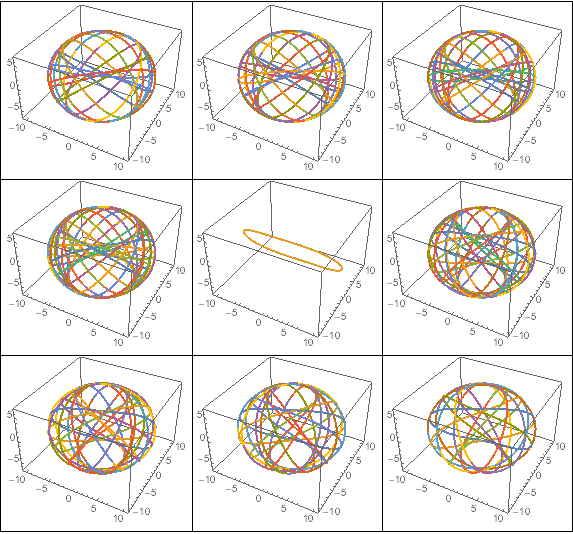
Figure 10. Trajectory of one of the bodies for some of the periodic solutions described in this paper.

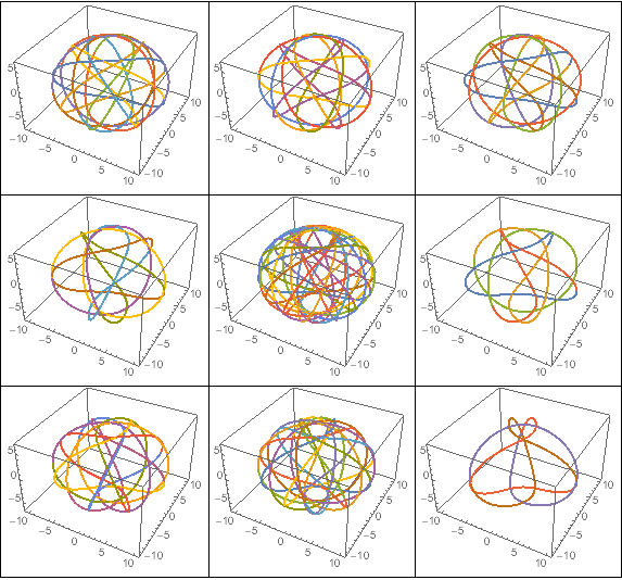
Figure 11. Trajectory of one of the bodies for some of the periodic solutions described in this paper.

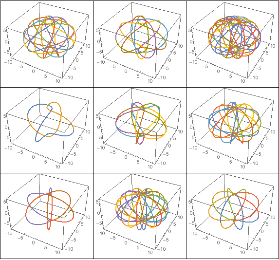
Figure 12. Trajectory of one of the bodies for some of the periodic solutions described in this paper.

References

- [1] Chenciner, A., Montgomery, R. A remarkable periodic solution of the three body problem in the case of equal masses. Annals of Math. 152 (2000), 881-901.
- [2] Gronwall, T. H. Note on the Derivatives with respect to a parameter of Solutions of a System of Differential Equations . Annals of Math. 20 (1919), 292-296.
- [3] Meyer, K. & Schmidt, D Libration of central configurations and braided saturn rings. Celestial Mechanics and Dynamical Astronomy 55: 289-303, 1993.
- [4] C. Moore Braids in Classical Gravity. Physical Review Letters 70 3675-3679.
- [5] H. Hénon A family of periodic solutions of the planar three-body problem, and their stability. Celestial Mechanics 13 (1976) pp. 267-285
- [6] Perdomo A family of solution of the n body problem. http://arxiv.org/pdf/1507.01100.pdf
- [7] Perdomo A small variation of the Taylor method and periodic solution of the 3-body problem. http://arxiv.org/pdf/1410.1757.pdf
- [8] Yan, D., Ouyang, T. New phenomenons in the spatial isosceles three-body problem. http://arxiv.org/abs/1404.4459