Study of multiband disordered systems using the typical medium dynamical cluster approximation

Abstract

We generalize the typical medium dynamical cluster approximation to multiband disordered systems. Using our extended formalism, we perform a systematic study of the non-local correlation effects induced by disorder on the density of states and the mobility edge of the three-dimensional two-band Anderson model. We include inter-band and intra-band hopping and an intra-band disorder potential. Our results are consistent with the ones obtained by the transfer matrix and the kernel polynomial methods. We apply the method to K_xFe_2-ySe₂ with Fe vacancies. Despite the strong vacancy disorder and anisotropy, we find the material is not an Anderson insulator. Our results demonstrate the application of the typical medium dynamical cluster approximation method to study Anderson localization in real materials.

I Introduction

The role of disorder (randomness) in materials has been at the forefront of current research Lee and Ramakrishnan (1985); Belitz and Kirkpatrick (1994); Abrahams (2010) due to the new and improved functionalities that can be achieved in materials by carefully controlling the concentration of impurities in the host. At half-filling and in the absence of any spontaneous symmetry breaking field, disorder can induce a transition in a non-degenerate electronic three-dimensional system from a metal to an insulator (MIT) Abrahams et al. (1979); Kramer and MacKinnon (1993). This phenomenon, which occurs due to the multiple scattering of charge carriers off random impurities, is known as Anderson localization Abrahams et al. (1979).

The most commonly used mean-field theory to study disordered systems is the coherent potential approximation (CPA) Soven (1967); Velický et al. (1968); Kirkpatrick et al. (1970), which maps the original disordered lattice to an impurity embedded in an effective medium. The CPA successfully describes some one-particle properties, such as the average density of states (ADOS) in substitutional disordered alloys Soven (1967); Velický et al. (1968); Kirkpatrick et al. (1970). However, being a single-site approximation, the CPA by construction neglects all disorder-induced nonlocal correlations involving multiple scattering processes. To remedy this, cluster extensions of the CPA such as the dynamical cluster approximation (DCA) Hettler et al. (2000); Jarrell and Krishnamurthy (2001); Jarrell et al. (2001) and the molecular CPA Tsukada (1969) have been developed, where nonlocal effects are incorporated. Unfortunately, all of these methods fail to capture the Anderson localization transition since the ADOS utilized in these approaches is neither critical at the transition or distinguish the extended and the localized states.

In order to describe the Anderson transition in such effective medium theories, a proper order parameter has to be used. As noted by Anderson, the probability distribution of the local density of states (LDOS) must be considered, and the most probable or typical value would characterize it Abrahams et al. (1979); Anderson (1978). It was found that the geometric mean of the LDOS is a good approximation of its typical value (TDOS) and it is critical at the transition Janssen (1998); Byczuk et al. (2010); Crow and Shimizu (1988), which makes it an appropriate order parameter to describe Anderson localization. Based on this idea, Dobrosavljevic et al. Dobrosavljević et al. (2003) formulated a single-site typical medium theory (TMT) for Anderson localization which gives a qualitative description of the transition in three dimensions. In contrast to the CPA, the TMT uses the geometrical averaging over the disorder configuration in the self consistency loop. And thus, the typical not the average DOS is used as the order parameter. However, due to the single-site nature of the TMT it neglects nonlocal correlations such as the effect of coherent back scattering. Thus, the TMT underestimates the critical disorder strength of the Anderson localization transition and fails to capture the reentrant behavior of the mobility edge (which separates the extended and localized states) for uniform box disorder.

Recently, a cluster extension of TMT was developed, named the typical medium dynamical cluster approximation (TMDCA) Ekuma et al. (2014), which predicts accurate critical disorder strengths and captures the reentrant behavior of the mobility edge. The TMDCA was also extended to include off-diagonal in addition to diagonal disorder. Terletska et al. (2014). However, like the TMT, the previous TMDCA implementations have only been developed for single-band systems, and in real materials, there are usually more than one band close to the Fermi level. Sen performed CPA calculation on two-band semiconducting binary alloys Sen (1973), and the electronic structure of disordered systems with multiple bands has also been studied numerically in finite systems Aoki (1981, 1985). But a good effective medium theory to study Anderson localization transition in multiband systems is still needed to understand the localization phenomenon in real systems such as diluted doped semi-conductors, disordered systems with strong spin-orbital coupling, etc.

In this paper, we extend the TMDCA to multiple band disordered systems with both intra-band and inter-band hopping, and study the effect of intra-band disorder potential on electron localization. We perform calculations for both single-site and finite size clusters, and compare the results with those from numerically exact methods, including transfer matrix method (TMM) and kernel polynomial method (KPM). We show that finite sized clusters are necessary to include the nonlocal effects and produce more accurate results. Since these results show that the method is accurate and systematic, we then apply it to study the iron selenide superconductor K_xFe_2-ySe₂ with Fe vacancies, as an example to show that this method can be used to study localization effects in real materials. In addition, as an effective medium theory, our method is also able to treat interactions Ekuma et al. (2015), unlike the TMM and KPM.

The paper is organized as follows. We present the model and describe the details of the formalism in Sec. II. In Sec. III.1, we present our results of the ADOS and TDOS for a two-band disordered system with various parameters, and use the vanishing of the TDOS to: determine the critical disorder strength, extract the mobility edge and construct a complete phase diagram in the disorder-energy parameter space for different inter-band hopping. In Sec. III.2, we discuss simulations of K_xFe_2-ySe₂ with Fe vacancies. We summarize and discuss future directions in Sec. IV. In Appendix A, we provide justification for the use of our order parameter ansatz.

II Formalism

II.1 Dynamical cluster approximation for multiband disordered systems

We consider the multiband Anderson model of non-interacting electrons with nearest neighbor hopping and random on-site potentials. The Hamiltonian is given by

$$\begin{split}H=&-\sum_{<ij>}\sum_{\alpha,\beta=1}^{l_{b}}t_{ij}^{\alpha\beta}(c_{i\alpha}^{\dagger}c_{j\beta}+c_{j\beta}^{\dagger}c_{i\alpha})\\ &+\sum_{i=1}^{N}\sum_{\alpha,\beta=1}^{l_{b}}(V_{i}^{\alpha\beta}-\mu\delta_{\alpha\beta})n_{i}^{\alpha\beta}\end{split}$$ (1)

The first term provides a realistic multiband description of the host valence bands. The labels $i$, $j$ are site indices and $\alpha,\beta$ are band indices. The operators $c_{i\alpha}^{\dagger}$($c_{i\alpha}$) create (annihilate) a quasiparticle on site $i$ and band $\alpha$. The second part denotes the disorder, which is modeled by a local potential $V_{i}^{\alpha\beta}$ that is randomly distributed according to some specified probability distribution $P(V_{i}^{\alpha\beta})$, where $n_{i}^{\alpha\beta}=c_{i\alpha}^{\dagger}c_{i\beta}$, $\mu$ is the chemical potential, and $t_{ij}^{\alpha\beta}$ are the hopping matrix elements. Here we consider binary disorder, where the random on-site potentials $V_{i}^{\alpha\beta}$ obey independent binary probability distribution functions with the form

$$P(V_{i}^{\alpha\beta})=x\delta(V_{i}^{\alpha\beta}-V_{A}^{\alpha\beta})+(1-x)\delta(V_{i}^{\alpha\beta}-V_{B}^{\alpha\beta}).$$ (2)

In our model, there are $l_{b}$ band indices so that both the hopping and disorder potential are $l_{b}\times l_{b}$ matrices. The random potential is

$$\underline{V_{i}}=\\ \left(\begin{array}[]{cccc}V_{i}^{\alpha\alpha}&\cdots&V_{i}^{\alpha\beta}\\ .&.&.\\ .&.&.\\ .&.&.\\ V_{i}^{\alpha\alpha}&\cdots&V_{i}^{\beta\alpha}\\ \end{array}\right),$$ (3)

while the hopping matrix is

$$\underline{t_{ij}}=\\ \left(\begin{array}[]{cccc}t_{ij}^{\alpha\alpha}&\cdots&t_{ij}^{\alpha\beta}\\ .&.&.\\ .&.&.\\ .&.&.\\ t_{ij}^{\beta\alpha}&\cdots&t_{ij}^{\beta\beta}\\ \end{array}\right),$$ (4)

where underbar denotes $l_{b}\times l_{b}$ matrix, $t^{\alpha\alpha}$ and $t^{\beta\beta}$ are intra-band hoppings, while $t^{\alpha\beta}$ and $t^{\beta\alpha}$ are inter-band hoppings. Similar definitions apply to the disorder potentials. If we restrict the matrix elements to be real, Hermiticity requires both matrices to be symmetric, i.e., $t^{\alpha\beta}=t^{\beta\alpha}$ and $V_{i}^{\alpha\beta}=V_{i}^{\beta\alpha}$.

To solve the Hamiltonian of Eq. 1, we first generalize the standard DCA to a multiband system. Within DCA the original lattice model is mapped onto a cluster of size $N_{c}=L^{3}$ with periodic boundary condition embedded in an effective medium. The first Brillouin zone is divided in $N_{c}$ coarse grained cells Jarrell and Krishnamurthy (2001), whose center is labeled by $K$, surrounded by points labeled by $\tilde{k}$ within the cell. Therefore, all the $k$-points are expressed as $k=K+\tilde{k}$. The effective medium is characterized by the hybridization function $\underline{\Delta(K,\omega)}$. The generalization of the DCA to a multiband system entails representing all the quantities in momentum space as $l_{b}\times l_{b}$ matrices.

The DCA self-consistency loop starts with an initial guess for the hybridization matrix $\underline{\Delta(K,\omega)}$, which is given by

$$\underline{\Delta(K,\omega)}=\\ \left(\begin{array}[]{cccc}\Delta^{\alpha\alpha}(K,\omega)&\cdots&\Delta^{\alpha\beta}(K,\omega)\\ .&.&.\\ .&.&.\\ .&.&.\\ \Delta^{\beta\alpha}(K,\omega)&\cdots&\Delta^{\beta\beta}(K,\omega)\\ \end{array}\right).$$ (5)

For the disordered system, we must solve the cluster problem in real space. In that regard, for each disorder configuration described by the disorder potential $V$ we calculate the corresponding cluster Green function which is now an $l_{b}N_{c}\times l_{b}N_{c}$ matrix

$$\underline{G}_{c}(V)=\left({\omega}\mathbb{I}-{\underline{t}^{(\alpha\beta)}}-{\underline{\Delta^{\prime}}^{(\alpha\beta)}}-{\underline{V}^{\alpha\beta}}\right)^{-1}\,.$$ (6)

Here, $\mathbb{I}$ is identity matrix and $\Delta_{ij}^{{}^{\prime}}$ is the Fourier transform (FT) of the hybridization, i.e.,

$$\Delta_{ij}^{{}^{\prime}\alpha\beta}=\sum_{K}\Delta^{\alpha\beta}(K)exp[iK\cdot(r_{i}-r_{j})].$$ (7)

We then stochastically sample random configurations of the disorder potential $V$ and average over disorder $\left\langle(\cdots)\right\rangle$ to get the $l_{b}N_{c}\times l_{b}N_{c}$ disorder averaged cluster Green function in real space

$$\underline{G_{c}(\omega)_{ij}}=\\ \left(\begin{array}[]{cccc}\left\langle G_{c}^{\alpha\alpha}(\omega,V)\right\rangle_{ij}&\cdots&\left\langle G_{c}^{\alpha\beta}(\omega,V)\right\rangle_{ij}\\ .&.&.\\ .&.&.\\ .&.&.\\ \left\langle G_{c}^{\beta\alpha}(\omega,V)\right\rangle_{ij}&\cdots&\left\langle G_{c}^{\beta\beta}(\omega,V)\right\rangle_{ij}\\ \end{array}\right)\,.$$ (8)

We then Fourier transform to $K$ space and also impose translational symmetry to construct the $K$-dependent disorder averaged cluster Green function $\underline{G_{c}(K,\omega)}$, which is a $l_{b}\times l_{b}$ matrix for each $K$ component

$$\underline{G_{c}(K,\omega)}=\\ \left(\begin{array}[]{cccc}G_{c}^{\alpha\alpha}(K,\omega)&\cdots&G_{c}^{\alpha\beta}(K,\omega)\\ .&.&.\\ .&.&.\\ .&.&.\\ G_{c}^{\beta\alpha}(K,\omega)&\cdots&G_{c}^{\beta\beta}(K,\omega)\\ \end{array}\right).$$ (9)

After the cluster problem is solved, we can calculate the coarse grained lattice Green function matrix

$$\underline{\overline{G}(K,\omega)} = \left(\begin{array}[]{cccc}\overline{G}^{\alpha\alpha}(K,\omega)&\cdots&\overline{G}^{\alpha\beta}(K,\omega)\\ .&.&.\\ .&.&.\\ .&.&.\\ \overline{G}^{\beta\alpha}(K,\omega)&\cdots&\overline{G}^{\beta\beta}(K,\omega)\\ \end{array}\right)$$

$$= \frac{N_{c}}{N}\sum_{\tilde{k}}\Big{(}\underline{G_{c}(K,\omega)}^{-1}+\underline{\Delta{}(K,\omega)}-\underline{\varepsilon_{k}}+\underline{\overline{\epsilon}(K)}\Big{)}^{-1},$$

where the overbar denotes cluster coarse-graining, and $\underline{\overline{\epsilon}(K)}$ is the cluster coarse-graining Fourier transform of the kinetic energy

$$\underline{\overline{\epsilon}(K)}=\underline{E_{0}}+\frac{N_{c}}{N}\sum_{\tilde{k}}\underline{\varepsilon_{k}}$$ (16)

where $E_{0}^{\alpha\beta}$ is a local energy, which is used to shift the bands. The diagonal components of Eq. II.1 have the same normalization than a conventional, i.e., scalar, Green function.

The DCA self-consistency condition requires the disorder averaged cluster Green function equal the coarse grained lattice Green function

$$\underline{G_{c}(K,\omega)}=\underline{\bar{G}(K,\omega)}.$$ (17)

Then, we close our self-consistency loop by updating the hybridization function matrix using linear mixing

$$\underline{\Delta_{n}(K,\omega)}=\underline{\Delta_{o}(K,\omega)}+\xi[\underline{G_{c}^{-1}(K,\omega)}-\underline{\bar{G}^{-1}(K,\omega)}],$$ (18)

where the subscript $``o"$ and $``n"$ denote old and new respectively, and $\xi$ is a linear mixing factor $0<\xi<1$. The procedure above is repeated until the hybridization function matrix converges to the desirable accuracy $\underline{\Delta_{n}(K,\omega)}=\underline{\Delta_{o}(K,\omega)}$.

We can see that when the inter-band hopping, $t^{\alpha\beta}$, and disorder potential, $V^{\alpha\beta}$, vanish all the $l_{b}\times l_{b}$ matrices become diagonal, and the formalism reduces to single band DCA for $l_{b}$ independent bands.

II.2 Typical medium theory for multiband disordered systems

To study localization in multiband systems, we generalize the recently developed TMDCA Ekuma et al. (2014) where the TDOS is used as the order parameter of the Anderson localization transition, so the electron localization is captured by the vanishing of the TDOS. We will use this TMDCA formalism to address the question of localization and mobility edge evolution in the multiband model.

Unlike the standard DCA, where the Green function is averaged over disorder algebraically, the TMDCA calculates the typical (geometrically) averaged cluster density of states in the self-consistency loop as

$$\rho_{c}^{typ}(K,\omega)=e^{\frac{1}{Nc}\sum_{i}\left\langle\log\rho_{ii}(\omega)\right\rangle}\left\langle\frac{\rho(K,\omega)}{\frac{1}{Nc}\sum_{i}\rho_{ii}(\omega)}\right\rangle,$$ (19)

which is constructed as a product of the geometric average of the local density of states, $\rho_{ii}=-\frac{1}{\pi}ImG_{ii}(\omega)$, and the linear average of the normalized momentum resolved density of states $\rho(K,\omega)=-\frac{1}{\pi}ImG_{c}(K,\omega)$. The cluster-averaged typical Green function is constructed via the Hilbert transformation

$$G_{c}^{typ}(K,\omega)=\int d\omega^{\prime}\frac{\rho_{c}^{typ}(K,\omega^{\prime})}{\omega-\omega^{\prime}}.$$ (20)

Generalization of the TMDCA to the multiband case is not straightforward since the off-diagonal LDOS $\rho_{ii}^{\alpha\beta}(\omega)=-\frac{1}{\pi}G_{ii}^{\alpha\beta}(\omega)$ is not positive definite. We construct the $l_{b}\times l_{b}$ matrix for the typical density of states as

$$\underline{\rho^{c}_{typ}(K,\omega)}=\\ \left(\begin{array}[]{cccc}e^{\frac{1}{Nc}\sum_{i}\left\langle ln\rho_{ii}^{\alpha\alpha}(\omega)\right\rangle}\left\langle\frac{\rho^{\alpha\alpha}(K,\omega)}{\frac{1}{Nc}\sum_{i}\rho_{ii}^{\alpha\alpha}(\omega)}\right\rangle&\cdots&e^{\frac{1}{Nc}\sum_{i}\left\langle ln|\rho_{ii}^{\alpha\beta}(\omega)|\right\rangle}\left\langle\frac{\rho^{\alpha\beta}(K,\omega)}{\frac{1}{Nc}\sum_{i}|\rho_{ii}^{\alpha\beta}(\omega)|}\right\rangle\\ .&.&.\\ .&.&.\\ .&.&.\\ e^{\frac{1}{Nc}\sum_{i}\left\langle ln|\rho_{ii}^{\beta\alpha}(\omega)|\right\rangle}\left\langle\frac{\rho^{\beta\alpha}(K,\omega)}{\frac{1}{Nc}\sum_{i}|\rho_{ii}^{\beta\alpha}(\omega)|}\right\rangle&\cdots&e^{\frac{1}{Nc}\sum_{i}\left\langle ln\rho_{ii}^{\beta\beta}(\omega)\right\rangle}\left\langle\frac{\rho^{\beta\beta}(K,\omega)}{\frac{1}{Nc}\sum_{i}\rho_{ii}^{\beta\beta}(\omega)}\right\rangle\\ \end{array}\right).$$ (21)

The diagonal part takes the same form as the single-band TMDCA ansatz, and the off-diagonal part takes a similar form but involves the absolute value of the off-diagonal ‘local’ density of states.

We construct the typical cluster Green function through a Hilbert transformation

$$\underline{G_{typ}^{c}(K,\omega)}=\\ \left(\begin{array}[]{cccc}\int d\omega^{\prime}\frac{\rho_{typ}^{\alpha\alpha}(K,\omega^{\prime})}{\omega-\omega^{\prime}}&\cdots&\int d\omega^{\prime}\frac{\rho_{typ}^{\alpha\beta}(K,\omega^{\prime})}{\omega-\omega^{\prime}}\\ .&.&.\\ .&.&.\\ .&.&.\\ \int d\omega^{\prime}\frac{\rho_{typ}^{\beta\alpha}(K,\omega^{\prime})}{\omega-\omega^{\prime}}&\cdots&\int d\omega^{\prime}\frac{\rho_{typ}^{\beta\beta}(K,\omega^{\prime})}{\omega-\omega^{\prime}}\\ \end{array}\right),$$ (22)

which plays the same role as $\underline{G_{c}(K,\omega)}$ in the DCA loop. Once $\underline{G_{typ}}$ is calculated from Eq. 22, the self-consistency steps are the same as those in the multiband DCA described in the previous section: we calculate the coarse grained lattice Green function using Eq. II.1, and use it to update the hybridization function matrix of the effective medium via Eq. 18.

The proposed ansatz Eq. 21 has the following properties. When the inter-band hopping $t^{\alpha\beta}$ and disorder potential $V^{\alpha\beta}$ vanish, it reduces to single-band TMDCA for $l_{b}$ independent bands, since all the off-diagonal elements of the Green functions vanish. When disorder is weak, all the $V^{\alpha\alpha}$ are small so the distribution of the LDOS becomes Gaussian with equal linear and geometric average so it reduces to DCA for a multiband disordered system.

When convergence is achieved, we use the total TDOS $\rho_{typ}^{tot}(\omega)$ to determine the mobility edge which is calculated as the trace of the local TDOS matrix

$$\rho_{typ}^{tot}(\omega)=Tr\left[\frac{1}{N_{c}}\sum_{K}\underline{\rho_{typ}(K,\omega)}\right]=\sum_{\forall\alpha=\beta}\rho_{typ}^{\alpha\beta}(\omega).$$ (23)

This construction of the order parameter may not seem very physical as the typical value of the LDOS should serve as the order parameter Abrahams et al. (1979); Anderson (1978), and the LDOS for the multiband system is the sum of the $l_{b}$ bands in the local site basis $\rho_{i}^{tot}=\sum_{\alpha=\beta}\rho_{i}^{\alpha\beta}(\omega)$. Therefore, the real order parameter should be the typical value of $\rho_{i}^{tot}$ defined as the geometric average of the total LDOS, $\exp(\frac{1}{N_{c}}\sum_{i}\log\rho_{i}^{tot})$ which is invariant under local unitary transformations and is not equal to the $\rho_{typ}^{tot}$ defined in Eq. 23.

However, Eq. 23 should also be a correct order parameter as long as it vanishes simultaneously with the typical value of $\rho_{i}^{tot}$, and we show this in Appendix A. By considering the distribution of the LDOS in each band, Appendix A shows that when localized states mix with extended states the system is still extended, which is consistent with Mott’s insight about the mobility edge Mott (1987). Intuitively, this makes sense as when all the distributions of $\rho_{i}^{\alpha\alpha}$ are critical then the typical values must behave as $~{}|V-V_{c}|^{\beta_{\nu}}$ near the transition, and so their sum must as well. If one is not critical (on the metallic side) then Eq. 23 will not vanish as $~{}|V-V_{c}|^{\beta_{\nu}}$, as expected.

To test our multiband typical medium dynamical cluster approximation formulation, we apply it to the specific case of a two band model, unless otherwise stated in Sec. III. Throughout the discussion of our results below, we denote $\alpha$ as $a$ and $\beta$ as $b$.

III Results

III.1 Two band model

As a specific example, we test the generalized DCA and TMDCA algorithms for a three-dimensional system with two degenerate bands (ab) described by Eq. 1. In this case, both the hopping and disorder potential are 2 $\times$ 2 matrices in the band basis given by

$$\underline{t_{ij}}=\underline{t}=\left(\begin{array}[]{cc}t^{aa}&t^{ab}\\ t^{ba}&t^{bb}\end{array}\right),$$ (24)

and

$$\underline{V_{i}}=\left(\begin{array}[]{cc}V_{i}^{aa}&V_{i}^{ab}\\ V_{i}^{ba}&V_{i}^{bb}\end{array}\right),$$ (25)

respectively. The intra-band hopping is set as $t^{aa}=t^{bb}=1$, with finite inter-band hopping $t^{ab}$. Here, the hopping matrix is defined as dimensionless so that the bare dispersion can be written as $\underline{\varepsilon_{k}}=\underline{t}\varepsilon_{k}$ with $\varepsilon_{k}=-2t[\cos(k_{x})+\cos(k_{y})+\cos(k_{z})]$ in three dimensions. We choose $4t=1$ to set the units of energy. We consider the two bands orthogonal to each other, where the local inter-band disorder $V_{i}^{\alpha\beta}$ vanishes and the randomness comes from the local intra-band disorder potential $V_{i}^{\alpha\alpha}$ that follow independent binary probability distribution functions with equal strength, $V^{aa}=V^{bb}$. Since the two bands are degenerate and the disorder strength for each band is also identical, the calculated average DOS will be the same for each band, so we only plot the quantities for one of the bands in the following results, as it is enough to characterize the properties of the system.

In our formalism, in order to disorder average instead of performing the very expensive enumeration of all disorder configurations, which scales as $2^{2N_{c}}$, we perform a stochastic sampling of configurations which greatly reduces the computational cost Ekuma et al. (2015). This is so we can study larger systems. For a typical $N_{c}=64$ calculation, 500 disorder configurations are enough to produce reliable results and this number decreases with increasing cluster size.

We first compare the ADOS and TDOS at various disorder strengths $V^{aa}(V^{bb})$, with a fixed inter-band hopping $t^{ab}=0.3$, for different cluster sizes $N_{c}$ in Fig. 1. Our TMDCA scheme for $N_{c}=1$ corresponds to the analog of the TMT for two-band systems, and the ADOS is calculated with the two-band DCA. To show the effects of non-local correlations introduced by finite clusters, we present data for both $N_{c}=1$ and $N_{c}>1$. We can clearly see that the TDOS, which can be viewed as the the order parameter of the Anderson localization transition, gets suppressed as the disorder increases . By comparing the width of the extended state region, where the TDOS is finite, we can see that single site TMT overestimates localization.

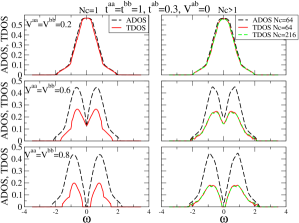
Figure 1: Evolution of the ADOS and TDOS at different disorder strengths $V^{aa}(V^{bb})$, for $N_{c}=1$ (left panel) and $N_{c}>1$ (right panel) for fixed $t^{ab}=0.3$. For small disorder, the ADOS and TDOS are almost identical. The TDOS is suppressed as the disorder increases. The extended states region with finite TDOS for $N_{c}=1$ is narrower than the results of $N_{c}>1$ which indicates that the single-site TMT overemphasizes localization.

From Fig. 1, we see that the results of TMDCA for $N_{c}=64$ and $N_{c}=216$ are almost on top of each other, showing a quick convergence with the increase of cluster size. To see this more clearly, we plot in Fig. 2 the TDOS at the band center for two different disorder strengths and various cluster sizes. We see that the results for both cases converge quickly with cluster size. Faster convergence (around $N_{c}=38$) is reached for the case further away from the critical region ($V^{aa}=V^{bb}=0.6$) than for the one closer ($V^{aa}=V^{bb}=0.7$) where convergence is reached around $N_{c}=98$. This is expected due to the critical slowing down close to the transition. To further study the convergence, we also plot in Fig. 3 the TDOS at the band center as a function of disorder strength ($V^{aa}=V^{bb}$) for several $N_{c}$. The critical disorder strength is defined by the vanishing of the TDOS($\omega=0$). The results show a systematic increase of the critical disorder strength as $N_{c}$ increases, and the convergence is reached at $N_{c}=98$ with the critical value of 0.74.

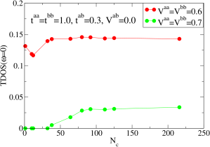
Figure 2: Evolution of the TDOS at the band center ($\omega=0$) with increasing cluster size for two different sets of parameters with $t^{aa}=t^{bb}=1.0$, $t^{ab}=0.3$, $V^{ab}=0.0$, $V^{aa}=V^{bb}=0.6,0.7$. The former has faster convergence (around $N_{c}=38$) than the latter (around $N_{c}=98$), due to the critical slowing down closer to the transition region.

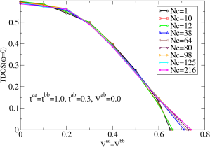
Figure 3: The TDOS at the band center ($\omega=0$) vs. $V^{aa}=V^{bb}$ with increasing cluster size, for $t^{aa}=t^{bb}=1.0$, $t^{ab}=0.3$, $V^{ab}=0.0$. For $N_{c}=1$, the critical disorder strength is 0.65 and as $N_{c}$ increases, it increases and converges to 0.74 for $N_{c}=98$.

To study the effect of inter-band hopping $t^{ab}$, we calculate the disorder-energy phase diagram for the case with vanishing $t^{ab}$ and finite $t^{ab}=0.3$ in Fig. 4. The mobility edge is determined by the energy where the TDOS vanishes. By comparing the left and right panels, we can see that introducing a finite $t^{ab}$ makes the system more difficult to localize, causing an upward shift of the mobility edge. The single site TMT overestimates the localized region compared to finite cluster results. We also compare our results with those from the TMM  Markos̆ (2006); MacKinnon and Kramer (1983); Kramer et al. (2010) to check the accuracy of the mobility edge calculated from TMDCA. For the TMM, the Schrödinger equation is written in terms of wavefunction amplitudes for adjacent layers in a quasi-one dimensional system, and the correlation (localization) length is computed by accumulating the Lyapunov exponents of successive transfer matrix multiplications that describe the propagation through the system. All TMM data is for a 3d system of length $L=10^{6}$ and the Kramer-MacKinnon scaling parameter $\Lambda(V,M)$ is computed for a given disorder strength $V$ and “bar” width $M$. The transfer matrix is a $2Ml_{b}\times 2Ml_{b}$ matrix. The system widths used were $M=[4-12]$. The critical point is found by identifying the crossing of the $\Lambda(M){\rm vs.}V$ curves for different system sizes. The transfer matrix product is reorthogonalized after every five multiplications.

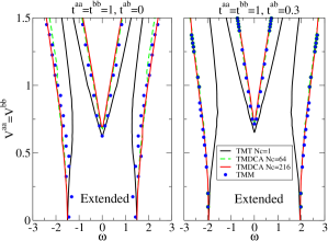
Figure 4: Disorder-energy phase diagram for vanishing $t^{ab}$ (left panel) and finite $t^{ab}=0.3$ (right panel). We compare the mobility edge obtained from the TMT ($N_{c}=1$), TMDCA ($N_{c}=64$ and $216$) and TMM. Parameters for the TMM data are given in the text (the TMM data for $t_{ab}=0.0$ is reproduced from  Terletska et al. (2014)). A finite $t^{ab}$ increases the critical disorder strength, indicating that $t^{ab}$ results in a delocalizing effect. The single site TMT overestimates the localized region.

To see the effect of inter-band hopping more directly, we now consider increasing $t^{ab}$ while keeping the disorder strength fixed ($V^{aa}=V^{bb}=0.71$), and study the evolution of the mobility edge (Fig. 5). The localized region around the band center starts to shrink as $t^{ab}$ is increased, leading to a small dome-like shape with the top located at $t^{ab}=0.2$. This shows that increasing $t^{ab}$ delocalizes the system which is reasonable since increasing $t^{ab}$ effectively increases the bare bandwidth.

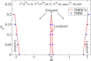
Figure 5: Evolution of the mobility edge as $t^{ab}$ increases, while $V^{aa}$ and $V^{bb}$ are fixed. The results are calculated for $N_{c}=64$. A dome-like shape shows up around the band center, signaling the closing of the TDOS gap. Parameters for the TMM data are given in the text.

To further benchmark our algorithms, we plot the ADOS and TDOS calculated with two-band DCA and TMDCA together with those calculated by the KPM Schubert and Fehske (2009); Weiße et al. (2006); Schubert et al. (2005); Schubert and Fehske (2008) (Fig. 6). In the KPM analysis, the LDOS is expanded by a series of Chebyshev polynomials, so that the ADOS and TDOS can be evaluated. The details for the implementation of KPM are well discussed in Ref. Weiße et al., 2006 and the parameters used in the KPM calculations are listed in the caption of Fig. 6. The Jackson kernel is used in the calculations Weiße et al. (2006). As shown in the plots, the results from the generalized DCA and TMDCA match nicely with those calculated from the KPM.

The excellent agreement of the TMDCA results with those from more conventional numerical methods, like KPM and TMM, suggest that the method may be used for the accurate study of real materials.

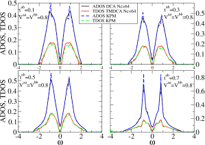
Figure 6: Comparison of ADOS and TDOS calculated with DCA, TMDCA and KPM with fixed disorder strength $V^{aa}=V^{bb}=0.8$ and various values of inter-band hopping $t^{ab}$. The KPM uses 2048 moments on a cubic lattice of size $48^{3}$ and 200 independent realizations generated with 32 sites randomly sampled from each realization.

III.2 Application to K_yFe_2-xSe₂

Next, we demonstrate the method with a case study of Fe vacancies in the Fe-based superconductor K_xFe_2-ySe₂, which has been studied intensely because of its peculiar electronic and structural properties. Early on it was found that there is a strong $\sqrt{5}\times\sqrt{5}$ ordering of Fe vacancies Wei et al. (2011). Later it was discovered that this material also contains a second phaseRicci et al. (2011); Wang et al. (2011). It is commonly speculated that the second phase is the one that hosts the superconducting state and the phase with the $\sqrt{5}\times\sqrt{5}$ vacancy ordering is an antiferromagnetic (AFM) insulator. Recent measurements of the local chemical composition Landsgesell et al. (2012); Ding et al. (2013) have determined that the second phase also contains a large concentration of Fe vacancies (up to 12.5%). However, these Fe vacancies are not well ordered since no strong reconstruction of the Fermi surface Lin et al. (2011); Berlijn et al. (2012); Cao and Zhang (2013) was observed by angle-resolved photoelectron spectroscopy (ARPES) experiments Chen et al. (2011); Zhang et al. (2011).

Interestingly, with such a disordered structure, this material hosts a relatively high superconducting transition temperature of 31 $K$ at ambient pressure Guo et al. (2010). It was the first Fe-based superconductor that was shown from ARPES Chen et al. (2011); Zhang et al. (2011) to have a Fermi surface with electron pockets only and no hole pockets, apparently disfavoring the widely discussed $S^{\pm}$ pairing symmetry Mazin et al. (2008) in the Fe-based superconductors. K_xFe_2-ySe₂ is also the only Fe-based superconductor whose parent compound (with perfectly ordered Fe vacancy) is an AFM insulator Fang et al. (2011) rather than a AFM bad metal. Furthermore from neutron scattering Wei et al. (2011), it has been observed that the anti-ferromagnetism has a novel block type structure with a record high Neel temperature of $T_{N}=559K$ and magnetic moment of 3.31$\mu_{B}$/Fe. Such a special magnetic structure is obviously not driven from the nesting of the simple Fermi surface, but requires the interplay between local moments and itinerant carriers present in the normal state Yin et al. (2010); Tam et al. (2015).

Given that Fe vacancies are about the strongest possible type of disorder that can exist in Fe-based superconductors and given that the Fe-based superconductors are quasi two-dimensional materials, it is natural to speculate how close the second phase is to an Anderson insulator. If it is indeed close, this would have interesting implications for the strong correlation physics and the non-conventional superconductivity in these compounds.

To investigate the possibility of Anderson localization in the second phase of K_xFe_2-ySe₂ we will employ TMDCA on a realistic first principles model. To this end we use Density Functional Theory (DFT) in combination with the projected Wannier function technique Ku et al. (2002) to extract the low energy effective Hamiltonian of the Fe-$d$ degrees of freedom. Specifically we applied the WIEN2K Schwarz et al. (2002) implementation of the full potential linearized augmented plane wave method in the local density approximation. The k-point mesh was taken to be $10\times 10\times 10$ and the basis set size was determined by RKmax=7. The lattice parameters of the primitive unit cell (c.f. Fig. 7(b)) are taken from Ref. Wei et al., 2011. The subsequent Wannier transformation was defined by projecting the Fe-d characters on the low energy bands within the interval [-3,2] eV. For numerical convenience, we use the conventional unit cell shown in Fig. 7(a) which contains 4 Fe atoms. Since there are 5 $d$ orbitals per Fe atom, we are dealing with a 20-band problem. To simulate the effect of Fe vacancies we add a local binary disorder with strength $V$ and Fe vacancy concentration $c_{a}$:

$$P(V_{i})=c_{a}\delta(V_{i}-V)+(1-c_{a})\delta(V_{i}).$$ (26)

We set the disorder strength to be $V=20eV$, much larger than the Fe-d bandwidth, such that it effectively removes the corresponding Fe-$d$ orbitals from the low energy Hilbert space. This will capture the most dominant effect of the Fe vacancies. The Fe concentration is taken to be $c_{a}=12.5\%$, which is the maximum value found in the experiments.

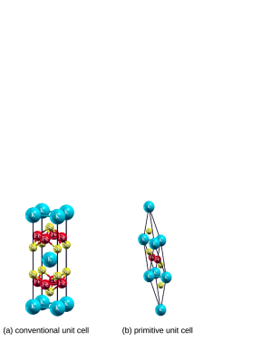
Figure 7: Crystal structure of KFe₂Se₂.

Fig. 8 presents the ADOS and TDOS, obtained from our multiband TMDCA for which we considered two cluster sizes $N_{c}=1$ and $N_{c}=2\sqrt{2}\times 2\sqrt{2}\times 2=16$. Consistent with the model calculations presented in the previous sections, we find that the TMT ($N_{c}=1$) tends to overestimate the localization effects compared to TMDCA results ($N_{c}=16$). While the TMT shows localized states within [0.6,1.1] eV, the TMDCA for $N_{c}=16$ finds localized states in the much smaller energy region [1.0,1.1] eV instead. Apparently a concentration of $c_{a}=12.5\%$ is still too small to cause any significant localization effects despite the strong impurity potentials of the Fe vacancies and the material being quasi-two dimensional. To determine the chemical potential we consider two fillings. The first filling of 6.0 electrons per Fe corresponds to the reported K₂Fe₇Se₈ phase Ding et al. (2013). Since strong electron doping has been found in ARPES experiments Chen et al. (2011); Zhang et al. (2011), we also consider a filling of 6.5 electrons per Fe. The latter would correspond to the extreme case of no vacancies. Clearly for both fillings the chemical potential remains energetically very far from the mobility edge, and thus far from Anderson insulating.

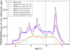
Figure 8: The average and typical density of states of KFe₂Se₂ with 12.5% Fe vacancy concentration calculated by multiband DCA and TMDCA with cluster size $N_{c}=1$ and $N_{c}=16$, compared with the average density of states of the clean (no vacancy) KFe₂Se₂.

IV Conclusion

We extend the single-band TMDCA to multiband systems and study electron localization for a two-band model with various hopping and disorder parameters. We benchmark our method by comparing our results with those from other numerical methods (TMM and KPM) and find good agreement. We find that the inter-band hopping leads to a delocalization effect, since it gradually closes the $\omega=0$ disorder induced gap on the TDOS. A direct application of our extended TMDCA could be done for disordered systems with strong spin-orbital coupling. Combined with electronic structure calculations, our method can be used to study the electron localization phenomenon in real materials. To show this, we apply this approach to the iron selenide superconductors K_xFe_2-ySe₂ with Fe vacancies. By calculating the TDOS around the chemical potential, we conclude that the insulating behavior of its normal state is unlikely due to Anderson localization. This method also has the ability to include interactions Ekuma et al. (2015), and future work will involve real material calculations that fully treat both disorder and interactions.

Acknowledgments– This work is supported in part by the National Science Foundation under the NSF EPSCoR Cooperative Agreement No. EPS-1003897 with additional support from the Louisiana Board of Regents (YZ, HT, CM, CE, KT, JM, and MJ). Work by TB was performed at the Center for Nanophase Materials Sciences, a DOE Office of Science user facility. This manuscript has been authored by UT-Battelle, LLC under Contract No. DE-AC05-00OR22725 with the U.S. Department of Energy. WK acknowledges support from U.S. Department of Energy, Office of Basic Energy Science, Contract No. DEAC02-98CH10886. The United States Government retains and the publisher, by accepting the article for publication, acknowledges that the United States Government retains a non-exclusive, paid-up, irrevocable, world-wide license to publish or reproduce the published form of this manuscript, or allow others to do so, for United States Government purposes. The Department of Energy will provide public access to these results of federally sponsored research in accordance with the DOE Public Access Plan (http://energy.gov/downloads/doepublic- access-plan). This work used the high performance computational resources provided by the Louisiana Optical Network Initiative (http://www.loni.org), and HPC@LSU computing.

Appendix A The order parameter defined in Eq. 23

We know the system is localized if the distribution of the total LDOS is critical, having a probability distribution $p(\rho_{i}^{aa}+\rho_{i}^{bb})$ which is highly skewed with a typical value close to zero. So if we can show that this is true if and only if both $\rho_{i}^{aa}$ and $\rho_{i}^{bb}$ are critical, then the critical behavior is basis independent and we can choose any particular basis and use the order parameter defined by Eq. 23 to study the localization transition.

To show this is true, we consider two probability distribution functions $p_{1}(x_{1})$ and $p_{2}(x_{2})$. The probability distribution function for $X=x_{1}+x_{2}$ is

$$P(X)=\int_{0}^{X}p_{1}(x)p_{2}(X-x)dx,$$ (27)

and we want to show $P(X)$ is critical if and only if both $p_{1}(x_{1})$ and $p_{2}(x_{2})$ are critical.

A.1 Sufficiency

If both $p_{1}(x)$ and $p_{2}(x)$ are critical, then both $p_{1}(x)$ and $p_{2}(x)$ are dominated by the region $0<x<\delta$ where $\delta\rightarrow 0^{+}$. The contribution to the integral in $P(X)$ mainly comes from the region $0<x<\delta$ and $0<X-x<\delta$ which is $max(X-\delta,0)<x<min(\delta,X)$. Since $\delta$ is infinitesimal, we can assume $X>\delta$, and then we have $X-\delta<x<\delta$. To maximize $P(X)$, we want this region to be as big as possible, so we want $\delta-(X-\delta)=2\delta-X$ to be as big as possible which means $X$ must be smaller than $2\delta\rightarrow 0^{+}$. Thus, $P(X)$ is also critical with the typical value around $2\delta$ which is infinitesimal.

A.2 Necessity

We now consider the case where one of the distributions is not critical. Without loss of generality, we assume $p_{2}(x)$ is not critical and is peaked at some finite value $x_{0}$. We calculate

$$\begin{split}P(x_{0})-P(\delta)&=\int_{0}^{x_{0}}p_{1}(x)p_{2}(x_{0}-x)dx-\int_{0}^{\delta}p_{1}(x)p_{2}(\delta-x)dx\\ &=\int_{0}^{\delta}p_{1}(x)[p_{2}(x_{0}-x)-p_{2}(\delta-x)]dx+\int_{\delta}^{x_{0}}p_{1}(x)p_{2}(x_{0}-x)dx.\end{split}$$ (28)

The first term is positive since $p_{2}(x)$ is peaked around $x_{0}$ and $\delta\ll x_{0}$. The second term is positive obviously, so $P(x_{0})>P(\delta)$. Therefore, $P(X)$ is not critical.

In this way we argue that $P(X)$ is critical if and only if both $p_{1}(x_{1})$ and $p_{2}(x_{2})$ are critical. In other words, when the localized states hybridize with extended states, only extended states remain which is exactly Mott’s insight about the mobility edge Mott (1987). The generalization to the multiple band case is trivial.

References

- Lee and Ramakrishnan (1985) P. A. Lee and T. V. Ramakrishnan, Rev. Mod. Phys. 57, 287 (1985).
- Belitz and Kirkpatrick (1994) D. Belitz and T. R. Kirkpatrick, Rev. Mod. Phys. 66, 261 (1994).
- Abrahams (2010) E. Abrahams, ed., 50 Years of Anderson Localization (World Scientific, 2010).
- Abrahams et al. (1979) E. Abrahams, P. W. Anderson, D. C. Licciardello, and T. V. Ramakrishnan, Phys. Rev. Lett. 42, 673 (1979).
- Kramer and MacKinnon (1993) B. Kramer and A. MacKinnon, Rep. Prog. Phys. 56, 1469 (1993).
- Soven (1967) P. Soven, Phys. Rev. 156, 809 (1967).
- Velický et al. (1968) B. Velický, S. Kirkpatrick, and H. Ehrenreich, Phys. Rev. 175, 747 (1968).
- Kirkpatrick et al. (1970) S. Kirkpatrick, B. Velický, and H. Ehrenreich, Phys. Rev. B 1, 3250 (1970).
- Hettler et al. (2000) M. H. Hettler, M. Mukherjee, M. Jarrell, and H. R. Krishnamurthy, Phys. Rev. B 61, 12739 (2000).
- Jarrell and Krishnamurthy (2001) M. Jarrell and H. R. Krishnamurthy, Phys. Rev. B 63, 125102 (2001).
- Jarrell et al. (2001) M. Jarrell, T. Maier, C. Huscroft, and S. Moukouri, Phys. Rev. B 64, 195130 (2001).
- Tsukada (1969) M. Tsukada, J. Phys. Soc. Jpn. 26, 684 (1969).
- Anderson (1978) P. W. Anderson, Rev. Mod. Phys. 50, 191 (1978).
- Janssen (1998) M. Janssen, Phys. Rep. 295, 1 (1998).
- Byczuk et al. (2010) K. Byczuk, W. Hofstetter, and D. Vollhardt, Int. J. Mod. Phys. B 24, 1727 (2010).
- Crow and Shimizu (1988) E. Crow and K. Shimizu, eds., Log-Normal Distribution–Theory and Applications (Marcel Dekker, NY, 1988).
- Dobrosavljević et al. (2003) V. Dobrosavljević, A. A. Pastor, and B. K. Nikolić, EPL 62, 76 (2003).
- Ekuma et al. (2014) C. E. Ekuma, H. Terletska, K.-M. Tam, Z.-Y. Meng, J. Moreno, and M. Jarrell, Phys. Rev. B 89, 081107 (2014).
- Terletska et al. (2014) H. Terletska, C. E. Ekuma, C. Moore, K.-M. Tam, J. Moreno, and M. Jarrell, Phys. Rev. B 90, 094208 (2014).
- Sen (1973) P. N. Sen, Phys. Rev. B 8, 5613 (1973).
- Aoki (1981) H. Aoki, Journal of Physics C: Solid State Physics 14, 2771 (1981).
- Aoki (1985) H. Aoki, Journal of Physics C: Solid State Physics 18, 2109 (1985).
- Ekuma et al. (2015) C. E. Ekuma, S.-X. Yang, H. Terletska, K.-M. Tam, N. S. Vidhyadhiraja, J. Moreno, and M. Jarrell, ArXiv e-prints (2015), arXiv:1503.00025 [cond-mat.dis-nn] .
- Mott (1987) N. Mott, J. Phys C 20, 3075 (1987).
- Ekuma et al. (2015) C. E. Ekuma, C. Moore, H. Terletska, K.-M. Tam, J. Moreno, M. Jarrell, and N. S. Vidhyadhiraja, Phys. Rev. B 92, 014209 (2015).
- Markos̆ (2006) P. Markos̆, Acta Physica Slovaca 56, 561 (2006).
- MacKinnon and Kramer (1983) A. MacKinnon and B. Kramer, Z. Phys. B 53, 1 (1983).
- Kramer et al. (2010) B. Kramer, A. MacKinnon, T. Ohtsuki, and K. Slevin, Int. J. Mod. Phys. B 24, 1841 (2010).
- Schubert and Fehske (2009) G. Schubert and H. Fehske, in Quantum and Semi-classical Percolation and Breakdown in Disordered Solids, Lecture Notes in Physics, Vol. 762, edited by B. K. Chakrabarti, K. K. Bardhan, and A. K. Sen (Springer Berlin Heidelberg, 2009) pp. 1–28.
- Weiße et al. (2006) A. Weiße, G. Wellein, A. Alvermann, and H. Fehske, Rev. Mod. Phys. 78, 275 (2006).
- Schubert et al. (2005) G. Schubert, A. Weiße, and H. Fehske, Phys. Rev. B 71, 045126 (2005).
- Schubert and Fehske (2008) G. Schubert and H. Fehske, Phys. Rev. B 77, 245130 (2008).
- Wei et al. (2011) B. Wei, H. Qing-Zhen, C. Gen-Fu, M. A. Green, W. Du-Ming, H. Jun-Bao, and Q. Yi-Ming, Chinese Physics Letters 28, 086104 (2011).
- Ricci et al. (2011) A. Ricci, N. Poccia, G. Campi, B. Joseph, G. Arrighetti, L. Barba, M. Reynolds, M. Burghammer, H. Takeya, Y. Mizuguchi, Y. Takano, M. Colapietro, N. L. Saini, and A. Bianconi, Phys. Rev. B 84, 060511 (2011).
- Wang et al. (2011) Z. Wang, Y. J. Song, H. L. Shi, Z. W. Wang, Z. Chen, H. F. Tian, G. F. Chen, J. G. Guo, H. X. Yang, and J. Q. Li, Phys. Rev. B 83, 140505 (2011).
- Landsgesell et al. (2012) S. Landsgesell, D. Abou-Ras, T. Wolf, D. Alber, and K. Prokeš, Phys. Rev. B 86, 224502 (2012).
- Ding et al. (2013) X. Ding, D. Fang, Z. Wang, H. Yang, J. Liu, Q. Deng, G. Ma, C. Meng, Y. Hu, and H.-H. Wen, Nat. Comm. 4 4, 1897 (2013).
- Lin et al. (2011) C.-H. Lin, T. Berlijn, L. Wang, C.-C. Lee, W.-G. Yin, and W. Ku, Phys. Rev. Lett. 107, 257001 (2011).
- Berlijn et al. (2012) T. Berlijn, P. J. Hirschfeld, and W. Ku, Phys. Rev. Lett. 109, 147003 (2012).
- Cao and Zhang (2013) C. Cao and F. Zhang, Phys. Rev. B 87, 161105 (2013).
- Chen et al. (2011) F. Chen, M. Xu, Q. Q. Ge, Y. Zhang, Z. R. Ye, L. X. Yang, J. Jiang, B. P. Xie, R. C. Che, M. Zhang, A. F. Wang, X. H. Chen, D. W. Shen, J. P. Hu, and D. L. Feng, Phys. Rev. X 1, 021020 (2011).
- Zhang et al. (2011) Y. Zhang, L. X. Yang, M. Xu, Z. R. Ye, F. Chen, C. He, H. C. Xu, J. Jiang, B. P. Xie, J. J. Ying, X. F. Wang, X. H. Chen, J. P. Hu, M. Matsunami, S. Kimura, and D. L. Feng, Nat Mater 10, 273 (2011).
- Guo et al. (2010) J. Guo, S. Jin, G. Wang, S. Wang, K. Zhu, T. Zhou, M. He, and X. Chen, Phys. Rev. B 82, 180520 (2010).
- Mazin et al. (2008) I. I. Mazin, D. J. Singh, M. D. Johannes, and M. H. Du, Phys. Rev. Lett. 101, 057003 (2008).
- Fang et al. (2011) M.-H. Fang, H.-D. Wang, C.-H. Dong, Z.-J. Li, C.-M. Feng, J. Chen, and H. Q. Yuan, EPL (Europhysics Letters) 94, 27009 (2011).
- Yin et al. (2010) W.-G. Yin, C.-C. Lee, and W. Ku, Phys. Rev. Lett. 105, 107004 (2010).
- Tam et al. (2015) Y.-T. Tam, D.-X. Yao, and W. Ku, Phys. Rev. Lett. 115, 117001 (2015).
- Ku et al. (2002) W. Ku, H. Rosner, W. E. Pickett, and R. T. Scalettar, Phys. Rev. Lett. 89, 167204 (2002).
- Schwarz et al. (2002) K. Schwarz, P. Blaha, and G. Madsen, Computer Physics Communications 147, 71 (2002), Proceedings of the Europhysics Conference on Computational Physics, Computational Modeling and Simulation of Complex Systems.