This report has not been submitted to a journal but is provided on astro-ph as a reference for other scientists who use IRIS data.

The O iv intercombination lines observed by IRIS between 1397 and 1407 Å provide useful density diagnostics. This document presents data that address two issues related to these lines:

1. the contribution of S iv to the O iv $\lambda$1404.8 line; and

2. the range of sensitivity of the O iv $\lambda$1399.8/$\lambda$1401.2 ratio.

1 Overview

O iv has a ground configuration of $2s^{2}2p$, and S iv a ground configuration of $3s^{2}3p$ and this similarity leads to common features in their spectra. In particular, each ion has a set of intercombination transitions of the form ${}^{2}P$–${}^{4}P$ where the upper state lies in the excited n$s$n$p^{2}$ configuration. There are five distinct transitions in these multiplets, and the O iv lines lie between 1397 and 1408 Å, and the S iv transitions lie between 1398 and 1424 Å (Table 1). The O iv multiplet is significantly stronger than the S iv multiplet in most conditions, and both sets of multiplets show density sensitivity in the $\log\,N_{\rm e}$=10–13 range.

Table 1: O iv and S iv transitions.

Ion	Wavelength	Transition	Comment
O iv	1397.198	1/2–3/2	weak line
	1399.766	1/2–1/2
	1401.157	3/2–5/2
	1404.779	3/2–3/2	blended with S iv
	1407.374	3/2–1/2	not observed by IRIS
S iv	1398.040	1/2–3/2	very weak line
	1404.808	1/2–1/2	blended with O iv
	1406.016	3/2–5/2
	1416.887	3/2–3/2	not observed by IRIS
	1423.839	1/2–3/2	not observed by IRIS

Since S iv is formed very close in temperature to O iv, then generally there is little interest in studying the S iv lines over the stronger O iv lines. However, one of the S iv lines blends with a useful O iv transition and so it is necessary to take account of this (Sect. 5).

The IRIS satellite (De Pontieu et al., 2014) observes the 1389.0–1407.0 Å wavelength band, although in practice the upper limit is $\approx$ 1406.6 Å. This means that a number of the transitions are not observed by IRIS (see Table 1 for details).

There have been many previous studies of the O iv and S iv lines due to their importance in both solar and stellar spectra, and Table 2 lists some key papers.

Table 2: Previous studies of the O iv intercombination lines.

Paper	Comment
Cook et al. (1995)	O iv and S iv lines in HRTS solar spectra and HST/GHRS spectra of Capella.
Harper et al. (1999)	O iv and S iv lines in HST/GHRS spectra of RR Tel.
Teriaca et al. (2001)	Densities in explosive events from SOHO/SUMER.
Keenan et al. (2002)	O iv and S iv lines in HST/STIS spectra of RR Tel, and SOHO/SUMER solar spectra.
Keenan et al. (2009)	O iv lines in stellar and solar spectra.

2 Atomic data

Atomic data for O iv and S iv used in this work are obtained from version 8 of the CHIANTI atomic database (Dere et al., 1997; Del Zanna et al., 2015). Radiative decay rates for the lowest 20 atomic levels (including the levels giving rise to the intercombination lines) of O iv were obtained from Corrégé & Hibbert (2004), and all other decay rates were taken from Liang et al. (2012). Effective collision strengths for all transitions were taken from Liang et al. (2012), although an error was corrected in these data, as reported in Del Zanna et al. (2015).

The S iv data-set has been unchanged since CHIANTI 5 (Landi et al., 2006), and consists of radiative decay rates from Hibbert et al. (2002), Tayal (1999), Johnson et al. (1986) and some unpublished data of P.R. Young. The data for the intercombination transitions are from Hibbert et al. (2002). Effective collision strengths for S iv are from Tayal (2000).

3 O IV Density sensitivity

Figure 1 shows the density sensitivity of the three O iv density diagnostic ratios that are important for IRIS. Temperature sensitivity is relatively small close to the temperature of maximum ionization of O iv ($\log\,T=5.15$), but in Figure 1 we show the ratios at $\log\,T=4.40$ at which there are relatively large differences. It is possible in non-equilibrium conditions that O iv could be formed closer to chromospheric temperatures (Olluri et al., 2013).

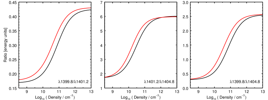
Figure 1: O iv ratio plots generated with CHIANTI 8. The black line has been calculated at $\log\,T=5.15$ and the red line at $\log\,T=4.4$.

4 IRIS spectra and calibration

In order to derive densities from the O iv density diagnostics, a number of spectra were selected and these are identified in Table 3. The spectra were chosen based on criteria such as: strength of the lines; lack of blending; symmetry of lines; and possibility of high density. The spectra were created using the IRIS_SUM_SPEC routine in Solarsoft. This routine sums blocks of pixels to create averaged spectra with error bars. For example, the IDL call to generate spectrum no. 8 is:

  IDL> file=iris_find_file(’12-oct-2013 21:34’)
  IDL> str=iris_sum_spec(file,xpix=9,ypix=[113,115],rnum=1)

The X-pixel and Y-pixel values for each spectra are given in Table 3, as well as the raster number (for data-sets in which multiple rasters were obtained). For each spectrum a background spectrum was subtracted from the feature spectrum by identifying a suitable background location near the feature along the slit direction. The Y-pixel values for the background spectra are given in Table 3 (the column “BG Ypix”). Note that the same X-pixel values as for the feature spectrum were used.

The background spectrum was subtracted from the feature spectrum, with the error arrays added in quadrature. Emission lines in the subtracted spectra were then fit with Gaussians using the IDL routine SPEC_GAUSS_WIDGET, which is also available in Solarsoft. Line intensities in data number (DN) units derived from the Gaussian fits are given in Table 5.

In this work we simply use the line intensities given in DN. The current version of the IRIS instrument response (implemented through the IDL routine iris_get_response) gives a completely flat response through the wavelength range of the O iv lines, and so the response function has no impact on line ratios. Note that densities are computed by using theoretical ratios given in photon units rather than energy units.

Table 3: Parameters used for computing spectra.

		Rast.			BG
Index	File start time	no.	Xpix	Ypix	Ypix	Comment
1	11-Oct-2013 23:54	0	238	471:475	460:464	S iv strong and fairly symmetric
2	11-Oct-2013 23:54	0	76:79	714:718	733:737	Supersonic loop footpoint; fit only supersonic component
3	11-Oct-2013 23:54	0	64	876:881	914:919	Bright, elongated structure
4	11-Oct-2013 23:54	0	92	710:714	658:662	Loop footpoint, not supersonic
5	10-Sep-2014 11:28	0	2321	338:341	344:346	Flare kernel site, narrow line
6	10-Sep-2014 11:28	0	1988:1992	491:492	481:485	Long loop structure; lines have weak, extended wings
7	10-Sep-2014 11:28	0	2381	301:304	309:313	Flare kernel, narrow lines, extended red wing
8	24-May-2014 06:10	0	25:32	532:545	–	South coronal hole, just above limb

The line intensities derived from the Gaussian fits are given in Table 5, and properties derived from the fits are given in Table 5. For the O iv $\lambda$1399.8/$\lambda$1401.2 ratio, we give the measured ratio and the corresponding density, derived from CHIANTI 8 assuming a temperature of $\log\,T=5.15$. The measured wavelength separation of the two lines is given in Table 5 which can be compared with the separation given by Young et al. (2011) of 1.391 Å. We also give the ratio of the width of $\lambda$1399.8 to that of $\lambda$1401.2, which gives an indication of the accuracy of the fits since the two lines should have the same widths. Large differences may indicate unaccounted for blending. The final column in Table 5 is the percentage contribution of S iv to the line at 1404.8 Å and this is discussed in the following section.

5 The 1404.8 line and S IV

The O iv $\lambda$1404.8 line is potentially a good density diagnostic relative to $\lambda$1401.1 (Fig. 1), but there is a known blend with S iv $\lambda$1404.8. The S iv contribution can be estimated through a branching ratio with $\lambda$1423.8, but this line is not observed by IRIS. An estimate can be made by considering $\lambda$1406.0, and this is discussed below.

Based on Skylab data, Feldman & Doschek (1979) found that S iv contributed 10% to the observed feature in quiet Sun conditions, but this rises to 33% in flare conditions. Cook et al. (1995) state that S iv contributes less than 10% by comparing the strength of the line against the nearby $\lambda$1406.1 transition. Teriaca et al. (2001) stated that S iv only contributed 3.6% to the observed feature in SUMER spectra but no details were given.

As IRIS does not observe the S iv $\lambda$1423.8 line, then we only have the $\lambda$1406.0 line to estimate the S iv contribution. Using CHIANTI 8 (Del Zanna et al., 2015), we find the $\lambda$1404.8/$\lambda$1406.0 ratio increases slightly with density, with values of 0.199, 0.202, and 0.224 at $\log\,N_{\rm e}$=9, 10, and 11, respectively. In Table 5 we multiply the $\lambda$1406 intensity, where available, by 0.210 and then divide this quantity by the $\lambda$1404.8 intensity to estimate the percentage contribution of S iv to the observed feature. We note that Cook et al. (1995) used the same method and they found the same correction factor (0.21) despite using much older atomic data.

The results demonstrate that S iv can make a significant contribution to the blended line and so we generally recommend not to use the 1404.8 Å line as part of a density diagnostic, unless the S iv $\lambda$1406.0 is also measured. We note, for example, that the IRIS flare line list does not include S iv $\lambda$1406.0. The $\lambda$1404.8 will be useful in low density data-sets, such as coronal holes and quiet Sun as $\lambda$1399.8 is weak in these regions, and so the $\lambda$1401.2/$\lambda$1404.8 ratio should give more precise results.

Table 4: Line intensities (DN).

	O iv			S iv
Spectrum	$\lambda$1399	$\lambda$1401	$\lambda$1404b	$\lambda$1406
1	$2576\pm 21$	$7499\pm 29$	$2239\pm 19$	$2738\pm 24$
2	$600\pm 8$	$2820\pm 11$	$1102\pm 9$	$179\pm 5$
3	$511\pm 13$	$1532\pm 15$	$622\pm 14$	$856\pm 14$
4	$256\pm 12$	$1093\pm 14$	$260\pm 13$	$62\pm 8$
5	$10375\pm 42$	$25491\pm 60$	$9750\pm 43$	—
6	$184\pm 6$	$627\pm 8$	$148\pm 6$	—
7	$847\pm 15$	$2119\pm 19$	$594\pm 15$	—
8	$142\pm 3$	$782\pm 3$	$360\pm 3$	$119\pm 2$

Table 5: Derived properties.

6 Blending lines for O IV 1399.8

In this and the following section we consider blending lines for O IV $\lambda$1399.8 and $\lambda$1401.2 that may affect density measurements from the $\lambda$1401.2/$\lambda$1399.8 ratio.

$\lambda$1399.8 is partly blended with a Fe ii line at 1399.960 Å and Fig. 2 shows an example where this line is quite strong, adding a narrow peak to the long wavelength side of the O iv line. Visually the line is about the same strength as Fe ii $\lambda$1401.777 which is close to O iv $\lambda$1401.2 (see Figure 2), and so this unblended line may be used to estimate whether the Fe ii contribution is important to O iv.

A more complex blending scenario can occur in flare ribbons, and Figure 3 shows an example spectrum for the 2014 September 10 X-flare in the vicinity of the O iv $\lambda$1399 line. The bright blob in the image is the O iv line, and one can see a number of very narrow features in the spectrum that have a larger extent in the Y-direction than the O iv line. The strongest of the displayed lines is at 1399.69 Å and, based on the intensity distribution along the slit, appears to be a H₂ line but the identification is not known. Care must be taken when deriving the intensity of O iv $\lambda$1399.8 from flare ribbons to estimate the strength of both this line and Fe ii $\lambda$1399.96.

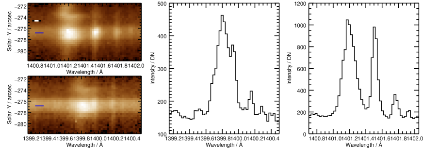
Figure 2: Spectra from an exposure obtained by a raster beginning at 22:08 UT on 2013 October 12. The left two panels show detector images around the O iv $\lambda$1399.8 (upper) and $\lambda$1401.2 (lower) lines, and the middle and right panel show spectra obtained at Y-pixel 114 (indicated by the short blue lines on the images.

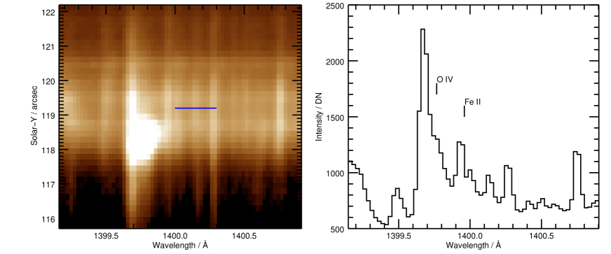
Figure 3: Spectrum for the 2014 September 10 X-flare. An exposure from X-pixel 2314 is shown in the left panel, and has been saturated to better show the weak lines. The O iv $\lambda$1399 line is the broad, bright structure. The blue line indicates the 1D spectrum shown in the right panel, which corresponds to Y-pixel 353.

7 Blending lines for O IV 1401.1

A commonly-seen line close to $\lambda$1401.1 is S i $\lambda$1401.514, although it is well-separated from the O iv line and generally not a problem (Fig. 2). Note that the velocity of the S i line relative to the O iv line is 76.4 km s^-1. Near sunspots strong supersonic downflows of $\approx$ 90 km s^-1 are often seen in the O iv line (Straus et al., 2015), and so the S i line can potentially be a problem when studying such flows, however the author’s experience is that S i is generally negligible in these structures.

8 The high density limit

Figure 4 shows the densities derived from the O iv $\lambda$1399.8/$\lambda$1401.2 ratio for each of the spectra identified in Table 3. The data span most of the density range of the ratio, from the coronal hole observation (spectrum 8) to the flare kernels (spectra 5 and 7). The fact that the measured ratios lie within the expected range of variation gives confidence in the atomic data for O iv. The 2014 September 10 X-flare does show examples of densities very close to $10^{12}$ cm^-3. We note that in features referred to as “bombs” by Peter et al. (2014), and also in flare kernels the O iv lines often become very weak or disappear. This was noted from Skylab data by Feldman & Doschek (1978) and was suggested to be due to densities that are so high that the O iv emitting levels are de-populated by electron collisions, reducing the strength of the lines. This would happen at $\approx 10^{13}$ cm^-3. The fact that densities of $\approx 10^{12}$ can be measured with the O iv ratio in later stages of flare kernel evolution suggests that higher densities may be feasible in the early stages of flares.

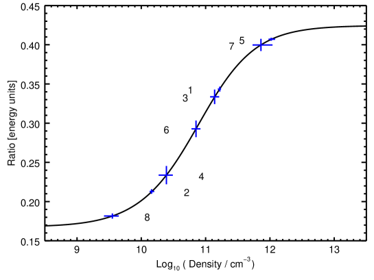
Figure 4: The solid line shows the theoretical variation of the O iv $\lambda$1399.8/$\lambda$1401.2 ratio as a function of density computed at $\log\,T=5.15$ using CHIANTI 8. The blue crosses show the measured ratios and densities with 1-$\sigma$ error bars. Numbers indicate the spectrum from which the measurements were made (Table 3).

As a sanity check on the extreme ratio values that were found in this analysis, Appendix A shows over-plots of the two O iv on top of each other.

9 Summary

The O iv density diagnostics observed by IRIS have been investigated and the following results found.

1. The line observed at 1404.8 Å is dominated by O iv but can contain a contribution from S iv up to 29% and so it is recommended that the S iv $\lambda$1406.0 line is observed in order to estimate the contribution.

2. The O iv $\lambda$1399.8 line is blended with an unknown line at 1399.69 Å, which is likely due to H₂. This line can be stronger than the O iv line in flare kernels.

3. A low density of $\log\,N_{\rm e}=9.5$ is measured just above the limb in a coronal hole.

4. In two flare kernel sites of the 2014 September 10 X-flare the density reached $\log\,N_{\rm e}=12$.

Appendix A Sanity check

To demonstrate that the low and high density limits of the O iv $\lambda$1399.8/$\lambda$1401.2 ratio are reached in the coronal hole and flare kernel data-sets, respectively, we show in Figure 5 the $\lambda$1399.8 and $\lambda$1401.2 line profiles over-plotted in velocity space, with the $\lambda$1401.2 profile scaled by the measured line ratio (Table 5).

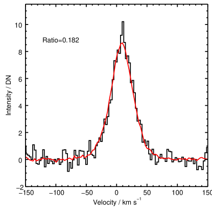
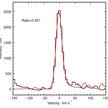
Figure 5: A comparison of the $\lambda$1399.8 (black) and $\lambda$1401.2 (red) spectral line profiles from spectrum 8 (left) and spectrum 5 (right). The $\lambda$1401.2 profile has been scaled by the measured ratio of the two lines, taken from Table 5.

References

- Cook et al. (1995) Cook, J. W., Keenan, F. P., Dufton, P. L., Kingston, A. E., Pradhan, A. K., Zhang, H. L., Doyle, J. G., & Hayes, M. A. 1995, ApJ, 444, 936
- Corrégé & Hibbert (2004) Corrégé, G., & Hibbert, A. 2004, Atomic Data and Nuclear Data Tables, 86, 19
- De Pontieu et al. (2014) De Pontieu, B., et al. 2014, Sol. Phys., 289, 2733
- Del Zanna et al. (2015) Del Zanna, G., Dere, K. P., Young, P. R., Landi, E., & Mason, H. E. 2015, ArXiv e-prints
- Dere et al. (1997) Dere, K. P., Landi, E., Mason, H. E., Monsignori Fossi, B. C., & Young, P. R. 1997, A&AS, 125, 149
- Feldman & Doschek (1978) Feldman, U., & Doschek, G. A. 1978, A&A, 65, 215
- Feldman & Doschek (1979) Feldman, U., & Doschek, G. A. 1979, A&A, 79, 357
- Harper et al. (1999) Harper, G. M., Jordan, C., Judge, P. G., Robinson, R. D., Carpenter, K. G., & Brage, T. 1999, MNRAS, 303, L41
- Hibbert et al. (2002) Hibbert, A., Brage, T., & Fleming, J. 2002, MNRAS, 333, 885
- Johnson et al. (1986) Johnson, C. T., Kingston, A. E., & Dufton, P. L. 1986, MNRAS, 220, 155
- Keenan et al. (2002) Keenan, F. P., et al. 2002, MNRAS, 337, 901
- Keenan et al. (2009) Keenan, F. P., Crockett, P. J., Aggarwal, K. M., Jess, D. B., & Mathioudakis, M. 2009, A&A, 495, 359
- Landi et al. (2006) Landi, E., Del Zanna, G., Young, P. R., Dere, K. P., Mason, H. E., & Landini, M. 2006, ApJS, 162, 261
- Liang et al. (2012) Liang, G. Y., Badnell, N. R., & Zhao, G. 2012, A&A, 547, A87
- Olluri et al. (2013) Olluri, K., Gudiksen, B. V., & Hansteen, V. H. 2013, ApJ, 767, 43
- Peter et al. (2014) Peter, H., et al. 2014, Science, 346, 1255726
- Straus et al. (2015) Straus, T., Fleck, B., & Andretta, V. 2015, ArXiv e-prints
- Tayal (1999) Tayal, S. S. 1999, Journal of Physics B Atomic Molecular Physics, 32, 5311
- Tayal (2000) Tayal, S. S. 2000, ApJ, 530, 1091
- Teriaca et al. (2001) Teriaca, L., Madjarska, M. S., & Doyle, J. G. 2001, Sol. Phys., 200, 91
- Young et al. (2011) Young, P. R., Feldman, U., & Lobel, A. 2011, ApJS, 196, 23