Magnetic ordering in quantum dots: Open vs. closed shells

Abstract

In magnetically-doped quantum dots changing the carrier occupancy, from open to closed shells, leads to qualitatively different forms of carrier-mediated magnetic ordering. While it is common to study such nanoscale magnets within a mean field approximation, excluding the spin fluctuations can mask important phenomena and lead to spurious thermodynamic phase transitions in small magnetic systems. By employing coarse-grained, variational, and Monte Carlo methods on singly and doubly occupied quantum dots to include spin fluctuations, we evaluate the relevance of the mean field description and distinguish different finite-size scaling in nanoscale magnets.

I Introduction

Nanoscale magnets are fascinating systems displaying phenomena at the boundary between classical and quantum physics. They reveal important implications for fundamental phenomena, such as macroscopic quantum tunnelingChudnovski1988:PRL ; Friedman1996:PRL ; Garanin1997:PRB , magnetic polaron formationSeufert2001:PRL ; Beaulac2009:S , tunable magnetismFernandez-Rossier2007:PRL ; Abolfath2008:PRL ; Abolfath2007:PRL , and strongly-correlated statesOszwaldowski2012:PRB , as well as potential applications in information storage and processing, arising from the superparamagnetic limitWasner:2012 , magnetic hardening induced by nonmagnetic moleculesRaman2013:N , spin-lasers,Chen2014:NN ; Zutic2014:NN and implementations of qubits.DiVincenzo 1995:S ; Thiele2014:S

Despite the significant differences between nanoscale magnets and their bulk counterparts, a mean-field description that could be suitable for bulk magnets in the thermodynamic limit, remains also widely used in describing magnetic ordering in nanostructures. Unfortunately, the appealing simplicity of the mean-field approximation (MFA) can often mask important phenomena. Neglecting thermodynamic spin fluctuations can lead to spurious thermodynamic phase transitions in small magnetic systems. Does that imply that the MFA cannot describe nanomagnets, or that there are situations in which MFA could yield valuable and unexplored insights?

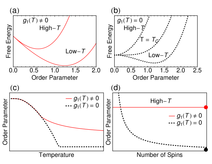
Figure 1: (Color online) Qualitative behavior of magnetic ordering in nanoscale systems. An example of a system that (a) does not and (b) does display a phase transition. The free energy, Eq. (1), is shown as a function of the order parameter at various temperatures applicable to both (a) and (b). (c) The temperature evolution of the order parameter for the free energy described in (a) and (b). (d) For high temperature, there are two qualitatively different finite-size scalings for the normalized order parameter which also extrapolate to distinct thermodynamic limits (circles).

In this work we show that the applicability of the MFA varies between different nanomagnets which also display different finite-size scaling and lead to distinct thermodynamic limits. We focus on magnetically-doped semiconductor quantum dots (QDs) with the localized impurity spins typically, provided by Mn ions.Maksimov2000:PRB ; Seufert2001:PRL ; Dorozhkin2003:PRB ; Holub2004:APL ; Besombes2004:PRL ; Hundt2005:PRB ; Gurung2008:APL ; Hoffman2000:SSC ; Norris2001:NL ; Radovanovic2001:JACS ; Beaulac2009:S ; Ochsenbein2009:NN ; Bussian2009:NM ; Zutic2009:NN ; Viswanatha2011:PRL ; Beaulac2011:PRB ; Pandey2012:NN ; Farvid2014:JACS ; Peng2014:JPC ; Xiu2010:ACSN ; Sellers2010:PRB ; Barman2015:PRB ; Henneberger:2010 ; Klopotowski2011:PRB ; Klopotowski2013:PRB ; Pacuski2014:CGD ; Kudelsk2007:PRL ; vanBree2008:PRB ; Govorov2004:PRB These systems are multi-carrier generalizations of the magnetic polaron formationYakovlev:2010 ; Dietl1982:PRL ; Wolff:1988 ; Durst2002:PRB ; Furdyna1988:JAP ; Nagaev:1983 ; Kasuya1968:RMP ; Dietl1995:PRL ; Awschalom1986:PRL that can be viewed as a cloud of localized impurity spins, aligned through exchange interaction with a confined carrier spin. The characteristic signatures of magnetic polarons is the presence of high-temperature tails in the root mean square magnetization, rather than an abrupt vanishing of magnetization at the Curie temperature, $T_{C}$, expected for bulk magnets.Marder:2010

To qualitatively distinguish magnetic ordering in different nanomagnets, such as epitaxially-grown or colloidal QDs,Hoffman2000:SSC ; Norris2001:NL ; Radovanovic2001:JACS ; Beaulac2009:S ; Ochsenbein2009:NN ; Zutic2009:NN ; Bussian2009:NM ; Viswanatha2011:PRL ; Beaulac2011:PRB ; Pandey2012:NN we introduce a simple description in which the relevant free energy functionalDietl1982:PRL ; Free_note is reduced to a MFA free energy, $F$, given as a function of the order parameter $X$, and the absolute temperature, $T$,

$$F(X,T)=g_{0}(T)+g_{1}(T)X+\frac{\alpha(T-T_{C})}{2}X^{2}+\frac{g_{4}(T)}{4}X^{4}.$$ (1)

where the expansion coefficients, $g_{0}$, $g_{1}$, $\alpha$, and $g_{4}$ are functions of $T$. The quadratic and quartic terms in $X$ describe the entropy of the magnetic ions. Compared to the conventional Ginzburg-Landau form,Marder:2010 it is surprising to see in Eq. (1) the linear term in $X$ in the absence of an applied magnetic field, we describe the origin of this term in Sec. III.

As shown in Fig. 1 (solid lines), the presence of a linear contribution in the order parameter, $g_{1}\neq 0$, has a striking consequence. For all relevant $T$,temp_note the free energy minimum is attained for a nonvanishing order parameter [Fig. 1(a)], implying the absence of a spurious phase transition. The magnetic order remains finite for all $T$ [Fig. 1(c)]. In contrast, for $g_{1}=0$ (broken lines) Figs. 1(b) and (c) reveal a behavior typically associated with bulk ferromagnets displaying a phase transition for $T>0$. Surprisingly, this simple MFA description provides two qualitatively different finite-size scaling with number of spins (magnetic ions) in Fig. 1(d) which we later show accurately reflects the behavior of two classes of nanoscale magnets by considering a more rigorous approach including spin fluctuations.

After this introduction, in Sec. II we provide an overview of the employed theoretical methods and discuss the importance of the correct choice of the order parameter. We then focus on the two classes of nanomagnets and the simplest magnetic QD embodiment: (i) a single occupancy, implying the finite carrier spin configuration of an open shell in Sec. III, and (ii) a double occupancy, corresponding to the vanishing carrier spin configuration of a closed shell in Sec. IV. We explain how these two classes of nanomagnets are already qualitatively different at the MF level corresponding to (i) $g_{1}\neq 0$ and (ii) $g_{1}=0$ behavior, in Fig. 1 and how they can be viewed as representing magnetic polaronsSeufert2001:PRL ; Beaulac2009:S ; Maksimov2000:PRB ; Sellers2010:PRB ; Barman2015:PRB ; Govorov2005:PRB ; Govorov2008:CRP ; Cheng2008:PRB and magnetic bipolarons,Oszwaldowski2012:PRB ; Oszwaldowski2011:PRL ; Bednarski2012:JPCM ; Abolfath2012:PRL respectively. We conclude our presentation with the implications for the relevance of MFA to nanomagnets and discuss outstanding questions.

II Theoretical Overview

Magnetically-doped QDs are a useful model system to study magnetic ordering in nanostructures. Even with very different growth techniques (top-town or bottom-up), such as epitaxially grown QDs or solution-processed colloidal QDs, there are striking similarities in the manifestations of their nanoscale magnetism, as well as in the limitations of their theoretical description. We illustrate different implications of magnetic ordering by focusing on (II,Mn)VI QDs, depicted in Fig. 2. These systems display carrier-mediated magnetism, extensively studied in bulk dilute magnetic semiconductors. Since Mn²⁺ is isovalent with group II ions, carriers must be created independently; for example, excitation of electron-hole pairs by interband absorption of light [Fig. 2(a)]. By changing the intensity of light can thus change the QD occupancy to realize both open- and closed-shell QDs. A realization of multiple occupancy in QDs is observed in various experiments.Cherenko2010:PSSB ; Gould2006:PRL ; Matsuda2007:APL ; Bansal2009:PRB ; Fisher2005:PRL ; Besombes2005:PRB ; Trojnar2013:PRB

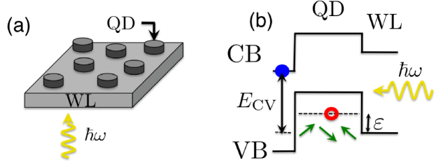
Figure 2: (Color online) (a) A scheme of QDs grown on a two-dimensional wetting layer (WL) in which electron-hole pairs are created by inter-band absorption of light. Holes are subsequently captured in the QD. Type-II conduction/valence band (CB/VB) profileKuskovsky2007:PRB of a II-VI QD doped with Mn spins.Sellers2010:PRB $\varepsilon$ and $E_{CV}$ are the confinement and bandgap energies.

From the band alignment of conduction and valence bands in Fig. 2(b), the ordering of Mn spins located in the QD region is dominated by the holes, characterized by the Mn-hole exchange coupling $\beta$. The electrons have a negligible influence on magnetic ordering. They are spatially removed from Mn and typically have $\sim$ 5-6 times smaller exchange coupling with Mn than holes.Furdyna1988:JAP

We first recall the MFA as known from bulk systems, but due to its simplicity it is often used in nanomagnets where its validity is questionable. A conventional mean-field theory is illustrated in Fig. 3, where the most probable state of the system is obtained by minimizing the free energy as a function of the order parameter. For nanoscale systems, one needs to be careful with the choice of an order parameter. This often overlooked consideration, has striking implications, as depicted in Fig. 3(a) and (b), which we further explain on the examples of magnetic polarons (MPs) and magnetic bipolarons (MBPs), discussed in Secs. III and  IV. A common choice of magnetization $\xi$ as the order parameter, shown in Fig. 3(a) leads to spurious thermodynamic phase transition in nanoscale magnets. In contrast, if an “observable” quantity, such as the exchange energy $X$, is chosen as the order parameter, the phase transition can be removed. This is shown in Fig. 3(b), where there is always a minimum in the free energy at all $T$. Based on the choice of the order parameter we can then recover either the $g_{1}=0$ or the $g_{1}\neq 0$ behavior of the free energy depicted in Figs. 1(a) and (b).

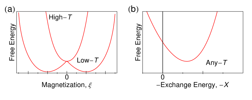
Figure 3: (Color online)  (a) The free energy as a function of magnetization, $\xi$, reveals a minimum at low-$T$ and vanishes at high-$T$. MFA will give a second-order phase transition. (b) Corrected free energy of a nanoscale magnet as a function of “observable” exchange energy, $X$, giving a finite value to the order for any finite $T$.

Some qualitative trends in magnetic QDs can be obtained from the MFA developed for bulk dilute magnetic semiconductors. The exchange coupling of a carrier (hole) and magnetic impurity (Mn) spins, $s$ and $S$, respectively, can be expressed in terms of two effective magnetic fields. The resulting self-consistent equations for the average spin (along the direction of the applied field or spontaneous Mn magnetization) are different depending on whether the carriers have nondegenerate or degenerate distribution DasSarma2003:PRB ; Petukhov2007:PRL . We will later discuss how these two bulk cases have similarities with the MFA applied to MPs and MBPs.

For nondegenerate carriers, the self-consistent equations are,Petukhov2007:PRL

$$\langle s_{z}\rangle=sB_{s}\left(\frac{\beta a_{0}^{3}n_{i}}{k_{B}T}\langle S_{z}\rangle\right),$$ (2)

$$\langle S_{z}\rangle=SB_{S}\left(\frac{\beta a_{0}^{3}n_{c}}{k_{B}T}\langle s_{z}\rangle\right),$$ (3)

where $a_{0}^{3}$ is the unit cell volume, $n_{c}$ and $n_{i}$ are the carrier and magnetic impurity densities, respectively; $k_{B}$ is the Boltzmann constant, and $B_{J}(x)$ is the Brillouin function,

$$B_{J}(x)=\frac{2J+1}{2J}\coth\left(\frac{2J+1}{2J}x\right)-\frac{1}{2J}\coth\left(\frac{x}{2J}\right).$$ (4)

In the high-$T$ limit of a small ratio of the effective magnetic and thermal energies, the expansion in Eq. (3),

$$B_{J}(x)\approx\frac{J+1}{3J}x+O(x^{3})\hskip 14.45377ptx\ll 1,$$ (5)

yields a vanishing magnetic response at a critical temperature,

$$k_{\text{B}}T_{C}=\frac{1}{3}\beta a_{0}^{3}\sqrt{n_{i}n_{c}}\sqrt{S(S+1)s(s+1)}.$$ (6)

For the degenerate case, the carrier spin is given by

$$\langle s_{z}\rangle = \frac{s}{2n_{c}}\int d\varepsilon f(\varepsilon)\left[D(\varepsilon+s\beta a_{0}^{3}n_{i}\langle S_{z}\rangle)\right.$$ (7)

$$- \left.D(\varepsilon-s\beta a_{0}^{3}n_{i}\langle S_{z}\rangle)\right].$$

where $D(\varepsilon)$ is the density of hole states. In the high-$T$ limit, the integrand in Eq. (7) can be expanded, using Eq. (3), and Eq. (5), to give the critical temperature

$$k_{\text{B}}T_{C}=\frac{1}{3}(\beta a_{0}^{3})^{2}n_{i}S(S+1)s^{2}D(\mu),$$ (8)

where $\mu$ is the chemical potential. Interestingly, the difference between the linear and quadratic $\beta$-dependence of the $T_{C}$ in MFA for the two bulk dilute magnetic semiconductors in Eq. (6) and (8) is also obtained using the MFA for MPs and MBPs, respectively.

At low-$T$, where spin fluctuations are small, MFA can accurately describe the thermodynamics of a finite-size system. However, a careful treatment is needed for a higher $T$, where large spin fluctuations could play the dominant role in the thermodynamics of magnetic QDs.Govorov2005:PRB ; Pientka2012:PRB

Unlike many studies of magnetic QDs that do not go beyond mean field theory,Abolfath2007:PRL ; Fernandez-Rossier2004:PRL ; Lebedeva2010:PRB ; Lebedeva2012:PSSB ; Abolfath2012:PRL we will utilize two methods which include spin fluctuations. The first is a coarse-grained approachOszwaldowski2012:PRB in which we discretize the QD space into a number of cells, $N_{c}$ with $N_{k}$ being the number of Mn spins belonging to each grid point where $\sum_{j=1}^{N_{k}}S_{jz}$ is the projection of the total spin onto the $z$-axis of the Mn contained at the $k^{\text{th}}$ grid point. Within a given cell the wave function is slowly varying allowing one to neglect the spatial dependence of the carrier and spin density. The full partition function is obtained by summing over all configurations of the normalized magnetization in a given cell.

The second method is to perform Monte Carlo simulations. Unlike the coarse-grained method, Mn can be positioned at many sites allowing for spatial variation in the carrier spin density. The Monte Carlo simulation seeks approximate solutions to the Schrödinger equation, for the Hamiltonian $\hat{H}$, at a fixed $T$, for a finite orthonormal basis $\ket{\Phi}$ at a given Mn spin $\{S_{z}\}$ configuration. The calculation entails randomly generating a Mn configuration at a given $T$ and producing a matrix representation of $\hat{H}(\{S_{z}\})$ in a finite basis and solving the eigenvalue problem. A metropolis algorithm is used to obtain the most probable Mn configuration at a fixed $T$.Binder:2009

Our model to study magnetic ordering in open- and closed-shell systems is motivated by the Mn-doped QD with type-II band alignment in Fig. 2, was shown experimentally to support robust MPs.Sellers2010:PRB We use the total QD Hamiltonian, $\hat{H}=\hat{H}_{c}+\hat{H}_{\mathrm{ex}}$, with typical two-dimensional (2D) nonmagnetic (carrier) and magnetic (Mn-hole exchange) parts, where

$$\hat{H}_{c}=\sum_{i=1}^{N_{h}}\left[-\frac{\hbar^{2}}{2m^{*}}\nabla_{i}^{2}+\frac{1}{2}m^{*}\omega^{2}r_{i}^{2}\right]+U_{N_{h}},$$ (9)

$\hbar$ is the Planck’s constant there are $N_{h}$ holes at the position ${\bf r}_{i}$ and $m^{\ast}$ is their effective mass. A harmonic $x-y$ confinement of strength $\omega$ is much weaker than the confinement along the growth ($z$) direction, implying effectively 2D system. $U_{N_{h}}$ is the charging energy. The $p-d$ exchange interaction between spins of Mn and confined holes has the Ising formDorozhkin2003:PRB ; Lee2014:PRB ; Stano2013:PRB ; Vyborny2012:PRB ; Gall2011:PRL because of the strong $z$-axis anisotropy, arising from spin-orbit interaction in the 2D QDs with energetically favorable heavy holes,

$$\hat{H}_{\rm{ex}}=-\frac{\beta}{3}\sum_{i=1}^{N_{h}}\sum_{j=1}^{N_{\text{Mn}}}\hat{s}_{zi}\hat{S}_{zj}\delta({\bf r}_{i}-{\bf R}_{j}),$$ (10)

where there are $N_{\text{Mn}}$ Mn spins at the position ${\bf R}_{j}$. Here, $\hat{s}_{z}$ is the heavy-hole (pseudo)spin operator with projections $s_{z}=\pm 3/2$, while $\hat{S}_{z}$ is the operator of the $z$-projection of the Mn-spin $S=5/2$. Our theory does not include antiferromagnetic interactions between neighboring Mn ions, which is relevant for QD’s doped with large Mn concentrationsKlosowsk1991:JAP .

Since $\hat{H}_{\mathrm{ex}}$ does not contain spin-flip processes, the total wave function is a product of the hole and Mn-spin parts.Wolff:1988 The partition function of the system can be calculated using a Gibbs canonical distribution,

$$Z=\text{Tr}_{S_{jz},s_{zi}}e^{-\hat{H}/k_{\text{B}}T},$$ (11)

which even for a single hole has a prohibitive complexity to be solved exactly. To calculate $Z$, in a typical QD with $N_{\text{Mn}}\sim 100-1000$ and $S$=5/2 for Mn spin, one would need to solve $6^{N_{\text{Mn}}}$ replicas of the hole Schrödinger equation.

To overcome this computational complexity and gain insight in magnetic ordering of open and closed-shell QDs we first use the MFA. We next consider a coarse-grained approach of discretizing the QD space to include spin fluctuations and examine the limitations of the MFA. We investigate the thermodynamics of the MP and the MBP formation and explore the finite-size effects by varying the number of magnetic impurity spins. We further corroborate our results and the influence of spin fluctuations using Monte Carlo simulations.

III Magnetic Polarons (MPs)

Early studies of MPs considered bulk magnetic semiconductors where the localized carrier spin was provided by the donor or acceptor.Nagaev:1983 ; Kasuya1968:RMP For such bound magnetic polarons a finite extent of the carrier wave function leads to the alignment of only a small number of a nearby spins of magnetic impurities having many similarities with MPs in magnetic QDs. While problems of a conventional MFA in describing experiments on bound magnetic polarons have been explained over thirty years ago,Dietl1982:PRL (spurious critical behavior and thermodynamic phase transitions in very small magnetic systems was removed after including spin fluctuations) such pitfalls continued to be repeated in describing magnetic QDs.

We begin by considering a singly occupied QD [$N_{h}=1$, $U_{N_{h}}=0$, recall Eqs. (9) and (10)], the simplest realization of an open-shell QD,note_open and study the thermodynamics of the MP. We build the partition function by constructing a canonical Gibbs distribution, Eq. (11). The distribution function, $\Omega_{S}(N_{k},\xi_{k})$, that describes the number of configurations of free spins in a given cell expressed in terms of the microscopic parameter, $\xi_{k}$ (which can be viewed as a normalized magnetization),

$$\Omega_{S}(N_{k},\xi_{k})=\sum_{\left\{S_{jz}\right\}}\ \delta\left(\xi_{k}-\frac{1}{N_{k}S}\sum_{j=1}^{N_{k}}S_{jz}\right),$$ (12)

where (recall Sec. II) $\sum_{j=1}^{N_{k}}S_{jz}$ is the projection of the total Mn spin onto the $z$-axis, and the argument of the $\delta$-function defines the normalization of $\xi$ while the $\delta$-function is the distribution of Mn spins in a cell. We find $\Omega_{S}(N_{k},\xi_{k})\propto\exp[-G_{S}(\xi_{k})/k_{\text{B}}T]$ (see Appendix A for details) with

$$G_{S}(\xi_{k})=k_{B}TN_{k}\left[\xi_{k}B_{S}^{-1}\left(\xi_{k}\right)-\ln Z_{S}\left(B_{S}^{-1}\left(\xi_{k}\right)\right)\right],$$ (13)

being the free energy for non-interacting spins, where $Z_{S}(x)=\sinh\left[(1+1/2S)x\right]/\sinh\left[x/2S\right]$, $B_{S}^{-1}(y)$ is the inverse of the Brillouin function $y=B_{S}(x)$. Kubo:1960

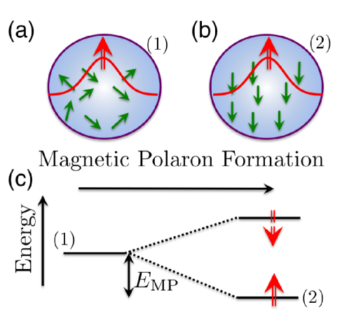
Figure 4: (Color online)  (a) A magnetic QD doped with random paramagnetic Mn ions (green arrow) with one carrier spin density (red arrow). (b) The system lowers its energy through the exchange interaction and results in an antiferromagnetic alignment between the hole spin and the Mn spins producing the MP. (c) The doubly degenerate QD energy level (1) splits with formation of the MP (2). The difference between the nonmagnetic QD energy and the ground state energy is the average exchange energy, $E_{\text{MP}}$.

A simple manifestation of a magnetic ordering in an open-shell QD occupied by a single carrier is the MP formation depicted in Fig. 4. Through exchange interactions between the carrier and Mn spins, once random paramagnetic Mn ions [Fig. 4(a)] acquire their spin alignment [Fig. 4(b)] (antiferromagetically coupled to a hole spin) and reduce the total energy of the carrier-Mn system. As a result of the hole-Mn exchange term in Eq. (10), the doubly degenerate heavy-hole energy level is split into two nondegenerate energy levels, as shown in Fig. 4(c). This corresponds to a red shift of the interband transition energy as a function of time, which is observed in time-resolved photoluminescence experiments.Seufert2001:PRL ; Beaulac2009:S ; Sellers2010:PRB ; Barman2015:PRB

In discrete space, for a given configuration of Mn spins, $\{\xi\}$, the two energy eigenvalues of Eq. (10) are, $E_{\pm}=\pm\Delta_{\text{MP}}/2$, with spin-splitting energy

$$\Delta_{\text{MP}}=\frac{2\beta}{3}S\sum_{k}N_{k}\rho_{\text{MP}}(R_{k})\xi_{k},$$ (14)

where,

$$\rho_{\text{MP}}(R_{k})=3|\phi(R_{k})|^{2}/2,$$ (15)

is the heavy hole spin density at the $k$’th cell, expressed in terms of the corresponding wave function $\phi$.

A MFA result for the spin-splitting energy $\Delta^{\rm MF}_{\text{MP}}$, is obtained by inter-relating the carrier and Mn spin densities $\langle s_{z}\rangle$ and $\langle\xi_{k}\rangle$, respectively, in analogy of Eqs. (2) and (3),

$$\langle{s_{z}}\rangle=\frac{3}{2}\tanh\left(\frac{3}{2}\sum_{k}\frac{\beta|\phi(R_{k})|^{2}}{3k_{B}T}N_{k}S\langle\xi_{k}\rangle\right),$$ (16)

and

$$\langle\xi_{k}\rangle=B_{S}\left(S\frac{\beta|\phi(R_{k})|^{2}}{3k_{B}T}\langle s_{z}\rangle\right).$$ (17)

Substituting Eq. (16) and (17) into Eq. (14) gives

$$\frac{\Delta^{\rm MF}_{\text{MP}}}{2}=\frac{\beta}{3}S\sum_{k}N_{k}\rho_{\text{MP}}(R_{k})B_{S}\left(\frac{\beta S\rho_{\text{MP}}(R_{k})}{3k_{B}T}\tanh\left[\frac{\Delta^{\rm MF}_{\text{MP}}}{2k_{B}T}\right]\right).$$ (18)

In the unsaturated limit, $\Delta^{\rm MF}_{\text{MP}}/2k_{B}T\ll 1$, Eq. (18) gives a vanishing $\Delta^{\rm MF}_{\text{MP}}$ at a critical temperature,

$$k_{\text{B}}T_{C,{\rm MP}}^{\rm MF}=\frac{\beta}{3}\left(\frac{S(S+1)}{3}\sum_{k}N_{k}\rho^{2}_{\text{MP}}(R_{k})\right)^{1/2}.$$ (19)

The MP energy, $E_{\text{MP}}$, is defined as the expectation value of Eq. (10). The MFA expression is

$$E_{\text{MP}}^{\text{MF}}=-\frac{\Delta^{\rm MF}_{\text{MP}}}{2}\tanh\left(\frac{\Delta^{\rm MF}_{\text{MP}}}{2k_{B}T}\right).$$ (20)

Having derived a MF theory description for the MP, one can make a connection between the MP and to that of a bulk nondegenerate magnetic semiconductors. Comparing Eqs. (19) and (6), we see in both cases that the critical temperature has a linear dependence on $\beta$. In a nondegenerate bulk semiconductor the concentration of donor/acceptor atoms is so small that the Pauli exclusion principle is ineffective and does not alter the carrier spin distribution which is described by the Boltzmann statistics. The magnetic impurity spins tend to align with one carrier spin and form a bound magnetic polaron.Nagaev:1983 The carrier spin in a nondegenerate magnetic semiconductor does not interact with other carriers spins. Thus, like the carrier in a magnetic QD, the carrier spins are free spins and will tend to align the spins of magnetic impurities.

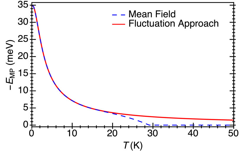
Figure 5: (Color online)  A mean field solution for MP blue/dashed curve and the result obtained through the fluctuation approach red/solid. For simplicity, we approximate the hole wave function as uniform throughout the QD volume $V$, $\phi(r)=1/\sqrt{V}$. Golnik1983:JPC The parameters are $N_{0}\beta$ = $-$1.05 eV, the cation density, $N_{0}=4/a_{0}^{3}$ with $a_{0}\simeq 6.1~{}$Å, $V=\pi r^{2}h_{z}$, $r=5$ nm, $h_{z}=2.5$ nm, $N_{\text{Mn}}=90$.

Next we turn our analysis to the MP energy. Motivated by typical QD parameters,Pientka2012:PRB the blue/dashed line in Fig. 5 shows the MF behavior of the MP energy Eq. (20) as a function of $T$. For the chosen parameters, MF predicts a second order phase transition at characteristic temperature $T_{C,{\rm MP}}^{\rm MF}=29$ K. The phase transition occurs at a $k_{B}T$ comparable to the exchange splitting of hole levels. At this temperature both hole states of opposite spin are approaching each other with equal probability. Consequently, yielding vanishing average MF spin density and average exchange energy at a finite $T$.

MFA neglects the possibility for the system to deviate from the minimum configuration, $\{\xi_{k}^{\rm MF}\}$, leading to phase transitions not allowed in nanoscale systems. To demonstrate the removal of the phase transition, we use the full partition function for the MP by summing over all configurations of $\{\xi_{k}\}.$Dietl1982:PRL The partition function is

$$Z_{\text{MP}}=\sum_{\sigma=\pm 1}\int\exp\left(\frac{\sigma\Delta_{\text{MP}}[\xi]}{2k_{B}T}\right)\prod_{k=1}^{N_{c}}\Omega_{S}(N_{k},\xi_{k})d^{N_{c}}\xi,$$ (21)

with the spin index $\sigma=\pm 1$ for the heavy-hole spin $s_{z}=\frac{3}{2}\sigma$. Since the distribution $\Omega_{S}(N_{k},\xi_{k})$ is an even function of $\xi_{k}$, the integrals for $\sigma=\pm 1$ yield the same result and

$$Z_{\text{MP}}=2\int\exp\left(\frac{\Delta_{\text{MP}}[\xi]}{2k_{B}T}\right)\prod_{k=1}^{N_{c}}\Omega_{S}(N_{k},\xi_{k})d^{N_{c}}\xi.$$ (22)

Here the summation of $\sigma=\pm 1$ is done exactly, without neglecting the statistical correlation between $\sigma$ and $\{\xi_{k}\}$ as in the MFA. Now, using the steepest descent method as above, we have

$$Z_{\text{MP}}=2\prod_{k=1}^{N_{c}}Z_{S}\left(\frac{\beta S\rho_{\text{MP}}(R_{k})}{3k_{B}T}\right)^{N_{k}}.$$ (23)

The average exchange energy can be evaluated from $E_{\rm MP}=-k_{B}T\beta d(\ln Z_{\rm MP})/d\beta$ as

$$E_{\text{MP}}=-\frac{\beta}{3}S\sum_{k}N_{k}\rho_{\text{MP}}(R_{k})B_{S}\left(\frac{\beta S\rho_{\text{MP}}(R_{k})}{3k_{B}T}\right),$$ (24)

where the corresponding results from Eq. (24) include the fluctuations of Mn spin and are compared in Fig. 5 (red/solid) with the MFA results (blue/dashed). In many colloidal QDs the number of magnetic impurities is much smaller than used in Fig. 5 ($N_{\text{Nm}}=90$), enhancing the importance of the fluctuations and the corresponding difference from the MFA solution.

The MP shows different behaviors in the high- and low-$T$ limits

$$E_{\rm MP}\propto\left\{\begin{array}[]{ll}-\beta&\mbox{ for }T\to 0\\ \\ -\beta^{2}/k_{B}T&\mbox{ for }\beta S\rho_{\rm MP}(R_{k})/k_{B}T\ll 1,\end{array}\right.$$ (25)

which correspond to saturated and unsaturated limits of magnetization, respectively. As shown in Fig. 5, $E_{\rm MP}$ has the $1/T$ behavior for a wide range of temperatures. This can be understood as follows. As depicted in Fig. 6, a single carrier with uncompensated spin couples to a sum of many Mn spins. Therefore the carrier aligns with the majority of Mn spin, and a flip of an individual Mn spin would not affect the carrier spin, and consequently other Mn spins. For this reason, the Mn spins are in effect weakly interacting which results in a $1/T$ Curie-like temperature dependence of $E_{\rm MP}$.

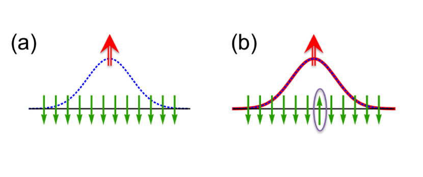
Figure 6: (Color online) Illustration of the finite-size effect for the MP (a) Spin density (blue/dashed) for fully aligned Mn spins (green). (b) A flipped Mn spin does not effect the carrier spin density (red/solid).

We now show that the MP does not display a finite-size effect, when in a fixed QD volume we change the number of Mn spins. Using the full MP partition function and the resulting Eq. (23), in Fig. 7(a) we show $E_{\text{MP}}(T)$, normalized with respect to its fully saturated value for various number of Mn. Figure 7(b) shows the normalized $E_{\text{MP}}$ plotted at fixed $T$ for various number of Mn ions. The normalized $E_{\text{MP}}$ remains constant. The finite size-effect was accurately predicted by the MFA. At the saturated and unsaturated limit, $E_{\rm MP}^{\rm MF}\propto N_{\text{Mn}}$. In Appendix B we show how $E_{\rm MP}$ will depend on a different choice of a carrier wave function.

To summarize, we interpret the previous calculations in terms of the Ginzburg-Landau approach of phase transitions. While the approach is not reliable due to the nanoscale size of our system, we may gain important insights. Typically the partition function is described by a functional integral over the magnetization $\xi$ [see Eq. (21)]. In the low-$T$ limit (or $|\Delta_{\text{MP}}|/2k_{B}T\gg 1$) with $e^{\Delta_{\text{MP}}/2k_{B}T}+e^{-\Delta_{\text{MP}}/2k_{B}T}\approx e^{|\Delta_{\text{MP}}|/2k_{B}T}$ in Eq. (21), one can write the free energy

$$F_{\text{MP}}(\xi)\approx-g_{1}|\xi|-k_{B}TS(\xi),$$ (26)

with the entropy $S(\xi)$ even in $\xi$. $F_{\text{MP}}(\xi)$ is depicted in Fig. 3(a). However, the finite potential barrier separating the degenerate minima at $\pm\xi_{\text{min}}$ does not prevent the thermal fluctuations between the local minima. Therefore the correct solution $\langle\xi\rangle=0$ is not predicted by the MFA to $F_{\text{MP}}(\xi)$.

We consider the Ginzburg-Landau approach defined with a different variable, the observable quantity of the exchange energy $X=E_{\text{ex}}=\sigma\Delta_{\text{MP}}/2$ [see Eq. (14)] with the carrier spin index $\sigma=\pm 1$. The linear dependence in $\xi$ originates from the finite carrier spin of the open shell. Since the carrier spin does not contribute to the entropy, the entropy in $X$ is directly related to $S(\xi)$, and we derive the free energy in the order parameter $X=E_{\text{ex}}$ as

$$F_{\text{MP}}(X)\approx X-TS(X),$$ (27)

as depicted in Fig. 3(b). Again, the entropy $S(X)$ is an even function of $X$ and Eq. (1) results for the magnetic polaron. Unlike $F_{\text{MP}}(\xi)$, $F_{\text{MP}}(X)$ possesses only one global minimum at a negative finite $X$ and $\langle X\rangle<0$ at all $T$, and the mean-field interpretation of Eq. (27) gives a qualitatively correct prediction. The thermodynamic solution of a finite $\langle X\rangle$ manifests itself in the finite-scale independence in $\langle X\rangle/N_{\text{Mn}}$ in Fig. 1(d).

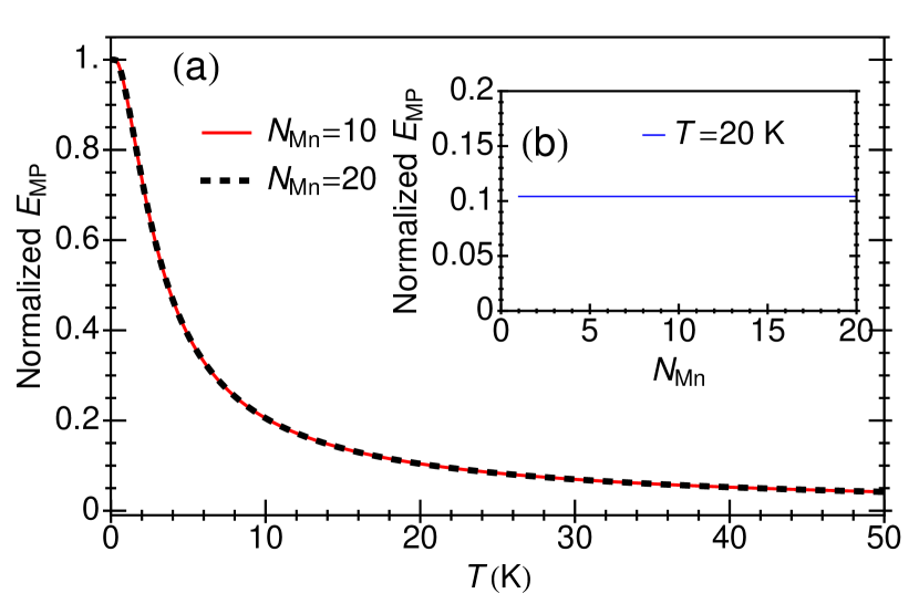
Figure 7: (Color online)  (a) The MP average exchange energy normalized by its $T=0$ K value for 10 Mn (red/solid) and 20 Mn (black/dashed) as function of $T$. (b) Normalized MP average exchange energy as a function of the total number of Mn at fixed $T$.

IV Magnetic Bipolarons (MBPs)

We next turn to a magnetic QD containing two holes [$N_{h}=2$, $U_{2}=U$, Eqs. (9) and (10)]. Closed-shell fermionic systems, such as noble gases, are known for their stability and the total spin-zero ground state, making them magnetically inert. Thus it would seem that this simple example of a two-hole closed-shell QD doped with Mn would not allow magnetic ordering. However, the Mn doping does alter the magnetic properties of closed-shell QDs. The corresponding ground state, which is neither a singlet nor a triplet, allows ordering of Mn spins, owing to the spontaneously broken time-reversal symmetry.Oszwaldowski2011:PRL

To lower the hole-Mn system energy through exchange interaction, there needs to be a nonvanishing hole spin density. During the MBP formation, an initially random Mn spin orientation [Fig. 8(a)], in the presence of two holes acquires a spin alignment [Fig. 8(b)]. The emergence of a nonvanishing local hole spin density, while the total hole spin density remains zero, is characteristic for a spin pseudosingletOszwaldowski2011:PRL ; Oszwaldowski2012:PRB , which can be understood from a simple perturbation picture. The exchange interaction admixes higher (single particle) orbitals to the ground-state $s$ orbital. Specifically, as shown in the Fig. 8(c), the mixing of $s$ and $p_{x}$ orbitals leads to the spin-Wigner molecule,Oszwaldowski2012:PRB a spin-analog of the Wigner molecule.Yannouleas2007:RPP ; Ghosal2006:NP ; Egger1999:PRL ; Ellenberger2006:PRL ; Singha2010:PRL ; Schinner2013:PRL In contrast to the Wigner molecule, where the spatial carrier separation originates from the Coulomb repulsion,Egger1999:PRL here the dominant contribution of such separation is typically the carrier-Mn exchange energy.

Figure 8: (Color online)  (a) A magnetic QD doped with random paramagnetic Mn ions spins (green arrows). (b) The system lowers its energy through the exchange interaction leading to a nonvanishing spin density and formation of the MBP. Red arrows and lines in (a) and (b) show how the two-carrier spin density changes due to the presence Mn. (c) The doubly occupied QD energy level (1) lowers its energy through the formation of the MBP (2). The difference between the nonmagnetic QD energy and the MBP ground state energy is the average exchange energy $E_{\text{ex}}$.

The corresponding pseudosinglet wave functionOszwaldowski2011:PRL at each snapshot of Mn configuration, $\{\xi_{k}\}$, is

$$\phi_{\text{PS}}(r_{1},r_{2})=\frac{N}{\sqrt{2}}\left[u(r_{1})d(r_{2})\ket{\uparrow;\downarrow}-u(r_{2})d(r_{1})\ket{\downarrow;\uparrow}\right],$$ (28)

where $N=1/(1+\varepsilon_{x}^{2})$ is the normalization constant, $u(r,\{\xi_{k}\})=s(r)+\varepsilon_{x}(\{\xi_{k}\})p_{x}(r)$, $d(r,\{\xi_{k}\})=s(r)-\varepsilon_{x}(\{\xi_{k}\})p_{x}(r)$, and $\varepsilon_{x}(\{\xi_{k}\})$ is a mixing (variational) parameter that depends on $\{\xi_{k}\}$. In choosing our variational wave function we neglect overlaps between like-orbitals, ($s-s$ and $p_{x}-p_{x}$), which results in the loss of fluctuations in the total magnetization at the site of Mn. These fluctuations are small in the MBP regime.

The variational energy $E(\varepsilon_{x})$ is

$$E=\frac{E_{s}+\varepsilon_{x}^{2}E_{p}}{1+\varepsilon_{x}^{2}}+U-\frac{\beta}{3}\sum_{j=1}^{N_{\text{Mn}}}\rho_{\text{MBP}}(R_{j},\varepsilon_{x})S_{j,z},$$ (29)

where the first term is the sum of the kinetic and potential energy, the second term is the Coulomb energy, taken to be constant, and the third term is the average exchange energy between the MBP spin density,

$$\rho_{\text{MBP}}(R_{j},\varepsilon_{x})=\frac{6\varepsilon_{x}}{1+\varepsilon_{x}^{2}}s(R_{j})p_{x}(R_{j}),$$ (30)

at the site of Mn. For a nonmagnetic system, the two-particle energy for the ground state is $E_{s}=2\hbar\omega$ and for the $p$-state is $E_{p}=4\hbar\omega$. To get close to the eigenstate of the system, we seek the $\varepsilon_{x}$ that minimizes Eq. (29)

$$\varepsilon_{x,\text{min}}=\frac{\Delta_{\rm MBP}}{E_{ps}/2+\sqrt{E_{ps}^{2}/4+\Delta_{\text{MBP}}^{2}}},$$ (31)

and minimized energy,

$$E_{\text{min}}=\frac{1}{2}\left(E_{s}+E_{p}-\sqrt{E_{ps}^{2}+4\Delta_{\text{MBP}}^{2}}\right)+U,$$ (32)

where $E_{ps}=E_{p}-E_{s}$ is the energy difference between the $s$ and $p_{x}$ orbital, and the spin splitting due to orbital polarization,

$$\Delta_{\text{MBP}}=\beta\sum_{j=1}^{N_{\text{Mn}}}s(R_{j})p_{x}(R_{j})S_{j,z}=E_{ps}\sum_{k=1}^{N_{C}}\chi_{k}\xi_{k},$$ (33)

with a dimensionless magnetic susceptibility like term

$$\chi_{k}=\frac{SN_{k}\beta s(R_{k})p_{x}(R_{k})}{E_{ps}}.$$ (34)

To obtain the full partition function we need to sum over all configurations of $\xi_{k}$. Since we are in the $k_{\text{B}}T\ll E_{ps}$ regime, we consider only the spin “singlet” ground state and neglect the possibility of a triplet state.note:triplet The partition function is

$$Z_{\text{MBP}}=\int e^{-E_{\text{min}}/k_{B}T}\prod_{k=1}^{N_{c}}\Omega_{S}(N_{k},\xi_{k})d^{N_{c}}\xi.$$ (35)

For simplicity, to evaluate Eq. (35), we use a two site model by placing $N_{k}$ Mn at two opposite sites equally spaced from the origin along the $x$-axis. The sites are chosen such that $s(R_{1})p_{x}(R_{1})=-s(R_{2})p_{x}(R_{2})$, where $R_{1}$ and $R_{2}$ are the position of the Mn ions at site 1 and site 2, respectively. For this two site problem, Eq. (33) reduces to $\Delta_{\text{MBP}}=E_{ps}\overline{\chi}\xi_{-}$, where

$$\xi_{-}=\xi_{2}-\xi_{1},$$ (36)

and $\overline{\chi}=|\chi_{1}|=|\chi_{2}|$, $N_{1}=N_{2}=N_{\rm Mn}/2$.

To investigate the MBP as a function of $T$, we begin by using the MFA. It can be shown that the minimum of the free energy, $F_{\text{MBP}}(\xi_{-})=E_{\text{min}}(\xi_{1},\xi_{2})+G_{S}(\xi_{1})+G_{S}(\xi_{2})$, lies on the $\xi_{1}=-\xi_{2}$ line. The free energy becomes

$$F_{\text{MBP}}(\xi_{-})=E_{\text{min}}(\xi_{-})+2G_{S}(\xi_{-}/2).$$ (37)

Minimization of the MBP free energy, Eq. (37), with respect to $\xi_{-}$ gives a self-consistent equation for $\Delta^{\rm MF}_{\text{MBP}}$,

$$\frac{\Delta^{\rm MF}_{\text{MBP}}}{2}=E_{ps}\overline{\chi}B_{S}\left(\frac{4\overline{\chi}\Delta^{\rm MF}_{\text{MBP}}}{N_{\rm Mn}k_{\text{B}}T\sqrt{E^{2}_{ps}+4(\Delta^{\rm MF}_{\text{MBP}})^{2}}}\right),$$ (38)

where $\Delta^{\rm MF}_{\text{MBP}}=E_{ps}\overline{\chi}\xi^{\rm MF}_{-}$. In the unsaturated limit, $\Delta^{\rm MF}_{\text{MBP}}/k_{B}T\ll 1$, Eq. (38) gives a vanishing $\Delta^{\rm MF}_{\text{MBP}}$ at a critical temperature,

$$k_{\text{B}}T_{C,{\rm MBP}}^{\rm MF}=\frac{8S(S+1)\overline{\chi}^{2}E_{ps}}{3N_{\rm Mn}}\propto\beta^{2}.$$ (39)

Unlike the MP, Eq. (19), the MF critical temperature for MBP is quadratic in $\beta$, through $\overline{\chi}^{2}$, a result similar to that of degenerate holes in bulk DMS, Eq. (8).

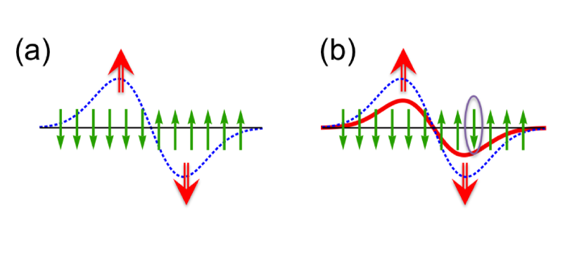
Figure 9: (Color online) Illustration of the finite-size effect for the MBP (a) Spin density (blue/dashed) for fully aligned Mn spins (green). (b) A flipped Mn spin changes the carriers spin density (red/solid).

We see that $\rho_{\text{MBP}}(\varepsilon_{x})$ in Eq. (30) is coupled linearly to the magnetic ordering of the Mn spins via Eqs. (31) and  (33), a result that is analogous to Pauli paramagnetism where the magnetization of a free electron gas is proportional to the strength of an external magnetic field. Thus, any small change in the Mn configuration will result in a linear response in the distribution of the carriers’ spin density. The strength of the response is determined by a Pauli-like susceptibly term given by Eq. (34). Figure 9(a) shows that one Mn spin “sees” the carrier orbital spin while one carrier spin “sees” all Mn collectively. Since the height of the spin density is determined by $\varepsilon_{x}$, which is dependent on the configuration of Mn spins, if one Mn spin changes, Fig. 9(b), the exchange field arising from the Mn field is strong that the carrier responds to the change. Therefore, inverting one Mn spin, Fig. 9(b), will change the amplitude of the spin density. Through the exchange interaction between the holes’ spin density and Mn spins, all other Mn will respond to the changing spin density. Thus, the Mn are indirectly interacting with one another through the hole.

The average exchange energy for the MBP is obtained the same way as the MP, using the solutions of Eq. (38) to give

$$E_{\text{ex}}^{\text{MF}}=\frac{-(\Delta^{\rm MF}_{\text{MBP}})^{2}}{\sqrt{E^{2}_{ps}/4+(\Delta^{\rm MF}_{\text{MBP}})^{2}}}.$$ (40)

The green/dashed line in Fig. 10(a) shows the $T$-dependence of Eq. (40), while Fig. 10(b) shows the mean field behavior of the averaged product of the normalized magnetization at the two sites, $\langle m_{2}m_{1}\rangle$. There is an antiferromagnetic correlation between the product of normalized magnetization at the two sites. As a consequence of thermal spin fluctuations, the average exchange energy and the magnitude of $\langle m_{2}m_{1}\rangle$ decreases and with increasing $T$ eventually vanishing when the MFA for the specific parameter set yields a vanishing carrier spin density resulting in a second order phase transition at $T_{C,{\rm MBP}}^{\rm MF}=1.5$ K.

Exact integration of the MBP partition function Eq. (35), which correctly includes spin fluctuations, is needed to remove the phase transitions predicted by MF theory. The average exchange energy is obtained through

$$E_{\text{ex}} = \frac{1}{Z_{\text{MBP}}}\int d\xi_{1}\int d\xi_{2}\Omega_{S}(N_{1},\xi_{1})\Omega_{S}(N_{2},\xi_{2})$$ (41)

$$\times \left[\beta\frac{\partial E_{\rm min}(\xi_{1},\xi_{2})}{\partial\beta}\right]e^{-E_{\text{min}}(\xi_{1},\xi_{2})/k_{\text{B}}T},$$

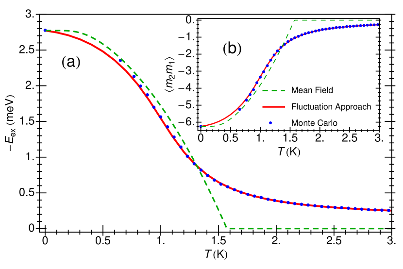
Figure 10: (Color online) (a) $T$-dependence of the average exchange energy and the removal of the phase transition for the two site model of the MBP, [Eq. (40)] with a non-fluctuating carrier spin density (green/dashed) and a fluctuating spin density (red/solid) [Eq. (41)]. (b) $T$-dependence of the product of magnetization of each site, $\langle m_{2}m_{1}\rangle$, for a fluctuating spin density (red/solid) and nonfluctuating spin density (green/dashed). The parameters are $h_{z}=2.5\text{ nm}$, $\hbar\omega=30\text{ meV}$, $m^{*}_{h}=0.21$, $N_{0}\beta$ = $-$1.05 eV, $U=30$ meV, $R_{1,2}=\pm 2$ nm and $N_{\rm Mn}=10$.

A $T$-dependence of this average exchange energy is shown by the red/solid lines in Fig. 10(a). With the inclusion of spin fluctuations, the phase transition is removed resulting in a finite $E_{\text{ex}}$ at $T>T_{C}$. The product of the normalized magnetization of each site was calculated numerically to demonstrate the antiferromagnetic correlation between the Mn spins at the two sites.

Monte Carlo simulations (see appendix C for details) verify the theoretical prediction for the MBP. $s-p$ levels coupled via Mn spins are directly diagonalized and the variational assumption, Eq. (28), was not used. Mn ions (5 per site) were placed 2 nm from the center of the QD along the $x$-axis. We include $s$, $p_{x}$ and $p_{y}$ orbitals in the simulation. The Coulomb energy, as before, is a constant. The blue dots in Fig. 10(a) shows the $T$-dependence of the average exchange energy and the product of the magnetization per site is shown in Fig. 10(b). There is an excellent agreement between the fluctuation approach and Monte Carlo simulations. Furthermore, the antiferromagnetic correlation between the two sites demonstrates the formation of the MBP.

As we did for the MP, we investigate two limiting cases for $E_{\text{ex}}$. In the saturated regime, the Mn are maximally aligned at each site with their spin pointing in opposite directions with $|\xi_{1}-\xi_{2}|\to 2$. In this limit, the MF expression, Eq. (40), is valid. In the opposite unsaturated high-$T$ limit, $e^{-E_{\rm min}(\xi_{1},\xi_{2})/k_{B}T}\approx 1$ can be taken in Eq. (41). Finally, we obtain the limiting behavior of $E_{\rm ex}$ within the regime $\overline{\chi}\ll 1$,

$$E_{\rm ex}\approx\left\{\begin{array}[]{ll}-6\frac{S}{S+1}N_{\rm Mn}T_{C,{\rm MBP}}^{\rm MF}\propto(N_{\rm Mn}\beta)^{2}&\mbox{ for }T\to 0\\ \\ -T_{C,{\rm MBP}}^{\rm MF}\propto N_{\rm Mn}\beta^{2}&\mbox{ for }T\to\infty\end{array}\right.$$ (42)

This shows that, unlike the MP, the coupling dependence is always in $\beta^{2}$. This is due to the fact that the carrier spin density is polarized from zero by the coupling to Mn spins, unlike the uncompensated carrier spin in the MP.

The MBP displays a finite-size effect different from the MP. We plot the $T$-dependence of the average exchange energy, Eq. (41), normalized by its low-$T$ value in Fig. 11(a) with a varying number of Mn in a given cell. As the number of Mn increases, the normalized $E_{\text{ex}}$ fluctuation tail decays toward the MF solution. This is demonstrated in Fig. 11(b) at a fixed ratio of $T/N_{\rm Mn}$. As the number of Mn ion spins increases toward the thermodynamic limit, the normalized exchange energy decays. This size dependence is expected from the MF result where a phase transition to zero exchange energy occurs. The $1/N_{\rm Mn}$ dependence in $E_{\rm ex}$ reflects the thermodynamic limit towards the vanishing order parameter.

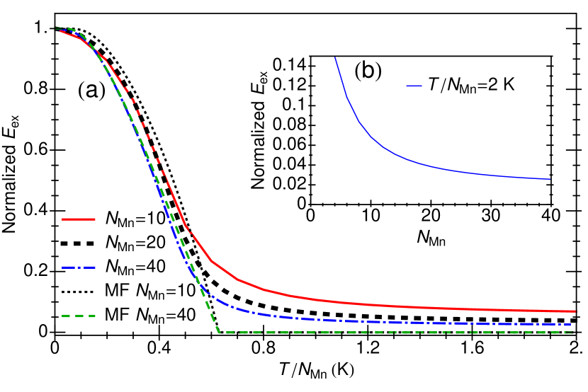
Figure 11: (Color online) The finite-size effect in a doubly occupied QD. (a) $T$-dependence of the normalized MBP average exchange energy for 10 Mn (red/solid), 20 Mn (black/dashed) and 40 Mn (blue/dash-dotted), thus 5, 10, and 20 Mn per site, respectively. Mean-field solution with 10 Mn (black/dotted) and 40 Mn (green/dashed). (b) The normalized mean-field solution with varying number of Mn for a fixed $T/N_{\rm Mn}$.

To summarize, like in the MP case, the MFA can be used to understand the statistical properties of the MBP. Applying the variational treatment to the carrier spins, we express the exchange energy as $E_{\text{ex}}=-a(\xi_{1}-\xi_{2})^{2}$ with the Mn spins $\xi_{1,2}$ at position 1 and 2. This quadratic dependence $(\xi_{1}-\xi_{2})^{2}$ originates from the carrier spin being linearly polarized out of the spin-singlet in closed-shell systems. With the variable $X\equiv\xi_{1}-\xi_{2}$, the free energy becomes

$$F_{\text{MBP}}(\xi_{1},\xi_{2})\approx-aX^{2}-TS(\xi_{1},\xi_{2}).$$ (43)

Confining the discussions to unpolarized states $(\xi_{1}+\xi_{2}=0)$, the entropy becomes an even function of $X$ and Eq. (1) results with $g_{1}=0$ [see Fig. 1(b)]. We note that, in contrast to the Eq. 1, here the first $X^{2}$ term in the free energy is not of an entropic origin. In a finite system $\langle X\rangle=0$ and the exchange energy $E_{\text{ex}}=-a\langle X^{2}\rangle$ remains finite. While the MFA incorrectly predicts a phase transition to $E_{\text{ex}}=0$ beyond a phase transition temperature, it correctly justifies the finite-size scaling limit $E_{\text{ex}}/N_{\rm Mn}\rightarrow 0$ as $N_{\rm Mn}\rightarrow\infty$ as shown in Fig. 1(d), in a sharp contrast to the MP case. The open or closed-shell electronic structures leads to fundamentally different statistical properties in the quantum dot magnetism.

V Conclusions

Many of our findings for magnetic polarons and bipolarons can be also applied to higher carrier occupancy of quantum dots where it is important to distinguish if they form open- or closed-shell systems which leads to a qualitatively different classes of magnetic ordering. Performing a thermodynamic analysis in these nanoscale magnets, we reveal the limitations of a mean-field approximation and the necessity for a more accurate theoretical framework that would correctly include spin fluctuations. Our results show that a careful choice of the order parameter in the mean-field approximation (using the exchange energy, rather than magnetization) removes spurious phase transitions for magnetic polarons, but not for magnetic bipolarons. In the later case, the phase transitions are removed by including spin fluctuations within the coarse-grained method and Monte Carlo simulations.

The conventional mean-field theory, known from bulk systems with nondegenerate or degenerate carrier density, reveals important differences between the magnetic polarons and bipolarons. Surprisingly, we can introduce a very simple mean-field form of a free energy to accurately describe qualitatively different finite-size effects and distinct thermodynamic limits in magnetic polarons and bipolarons with the change of the number of magnetic impurity spins. These findings remain unchanged once we carefully include spin fluctuations, further justifying our simple description and a pictorial difference between the finite-size effects in magnetic polarons and bipolarons, Figs. 6 and 9, respectively.

Similar to our prediction for an unexpected thermally-enhanced magnetic ordering in quantum dots,Pientka2012:PRB a judicious use of the mean-field approximation and awareness of its artifacts could provide important insights in unexplored aspects of nanoscale magnets. For example, we expect that the mean-field description of the different finite-size scaling in magnetic order discussed for magnetic polaron and bipolaron will also apply to other open- and closed shell quantum dots with higher carrier occupancy. A mean-field calculation of the critical temperature could also reveal a different power-law dependence in the exchange coupling constant for the exchange energy of open- and closed-shell systems.

In contrast to magnetic polarons, much less is known about magnetism in closed-shell systems, often simply implying that the magnetic ordering is completely absent. Therefore, to test our predictions for magnetic bipolarons it would be important to focus on the experimental realization of multiple carrier occupancy in quantum dots. The simple creation of excitons is not sufficient. A simultaneous presence of single electron and hole effectively just renormalizes the exchange coupling with magnetic impurities of magnetic polarons.Yakovlev:2010 Instead, photoexcitiation, using chemical and electrostatic doping,note_field should create a pair of holes or electrons.

Another possibility would be to fabricate quantum dots from novel Mn-doped II-II-V dilute magnetic semiconductors. These systems provide an independent charge and spin doping and would therefore be suitable to test formation of nanoscale magnetism for a wide range of parameters.Zhao2013:NC ; Zhao2014:CSB ; Glasbrenner2014:PRB They share with (II,Mn)VIs an isovalent character of Mn-doping, removing the solubility constraint of (III,Mn)Vs an obstacle for fabricating magnetic quantum dots.Kudelsk2007:PRL Unlike (II,Mn)VI, Mn-doped II-II-V systems can separately attain different carrier densities through independent charge doping and thus readily alter the strength of the Mn-carrier exchange coupling.

VI acknowledgements

We thank Peter Stano for discussions about the stability of magnetic bipolarons and Alex Matos Abiague for his valuable comments. This work was primarily supported by the U.S. DOE-BES, Office of Science, under Award DE-SC0004890 (I.Ž.), as well as grants U.S. ONR N000141310754 (J.P.), and NSF-DMR 0907150 (J.H).

Appendix A Mn Distribution Function

We discretize the QD space with $N_{k}$ magnetic moments in a given cell. The distribution function is found by summing over all configurations of the Mn in a given cell and is determined by Eq. (12). Using the integral representation of the $\delta$-function, $\delta(x)=(1/2\pi)\int_{-\infty}^{\infty}d\lambda e^{-i\lambda x}$, the partition function is

$$\Omega_{S}(N_{k},\xi_{k})=\frac{N_{k}S}{2\pi}\sum_{\left\{S_{jz}\right\}}\ \int_{-\infty}^{\infty}d\lambda e^{-i\lambda\left(N_{k}S\xi_{k}-\sum_{j=1}^{N_{k}}S_{jz}\right)}$$ (44)

Introducing a complex variable $h=i\lambda S$, Eq. (44) becomes

$$\Omega_{S}(N_{k},\xi_{k})=\frac{N_{k}}{2\pi i}\int_{-i\infty}^{i\infty}e^{N_{k}\left(\ln Z_{S}(h)-h\xi_{k}\right)}dh,$$ (45)

where $Z_{S}(x)=\sinh\left[(1+1/2S)x\right]/\sinh\left[x/2S\right]$. The integrand in Eq. (45 ) is sharply peaked (Gaussian-like), therefore we can approximate Eq. (45) by performing the method of steepest descent. We deform the contour in the complex plane to pass through a saddle point in the direction of steepest descent. By Taylor expansion of the function in the exponent of Eq. (45) and performing a Gaussian integral over $h$ we obtain

$$\Omega_{S}(N_{k},\xi_{k})=\sqrt{\frac{N_{k}}{2\pi\chi(h_{k})}}e^{-G_{S}(\xi_{k},T)/k_{B}T},$$ (46)

where $\chi(h)=\partial^{2}\ln Z_{S}(h)/\partial h^{2}$ and $G_{S}(\xi_{k},T)$ is the Gibbs free energy, recall Eq. (13), obtained through a Legendre transformation.Petukhov2007:PRL

Appendix B Magnetic Polaron Renormalization

Since the MP is not influenced by the finite-size effect (recall Figs. 6 and 7), we can employ a variational approach to study the influence of the wave function renormalization on the MP properties in a QD. Starting from the MP partition function in Eq. (23), we approximate the MP wave function by a single $s$-orbital of a 2D harmonic oscillator, constant over the the QD height, $h_{z}$,

$$\phi(r)=1/(\sqrt{h_{z}\pi}L_{\text{MP}})e^{-(x^{2}+y^{2})/2L_{\text{MP}}^{2}}.$$ (47)

Using a variational approachDietl1982:PRL ; Wolff:1988 we determine the width, $L_{\text{MP}}$, that minimizes the total free energy functional, $F_{\text{MP}}$. The MP free energy functional is given by

$$F_{\text{MP}} = \frac{\hbar\omega}{2}\left(\frac{L_{0}^{2}}{L_{\rm MP}^{2}}+\frac{L_{\rm MP}^{2}}{L_{0}^{2}}\right)-k_{\text{B}}T\ln 2$$ (48)

$$- k_{\text{B}}T\sum_{j=1}^{N_{\text{Mn}}}\ln\left[Z_{S}\left(\frac{\beta S\rho_{\mathrm{MP}}(R_{j})}{3k_{\text{B}}T}\right)\right],$$

where the first two terms are the sum of the kinetic and potential energy with $L_{0}=\sqrt{\hbar/m^{*}\omega}$, the third term is from the hole spin degeneracy, and the final term is due to the exchange interaction of the hole spin density $\rho_{\mathrm{MP}}(r)$ at the site of Mn spins, $R_{j}$. As an approximation, we consider a homogeneous distribution of Mn, and transform $\sum_{j}\rightarrow N_{0}x_{\text{Mn}}\int d^{3}R$ (the continuous limit) where $x_{\rm Mn}$ is the Mn fraction per cation and $N_{0}$ is the density of cation sites. The average exchange interaction for the MP, $E_{\text{MP}}$, can be derived to obtain

$$E_{\text{MP}}=-\frac{\Delta_{\text{max}}}{3}\int d^{3}R\rho_{\mathrm{MP}}(R)B_{S}\left(\frac{\beta S\rho_{\text{MP}}(R)}{3k_{\text{B}}T}\right),$$ (49)

where $\Delta_{\text{max}}=x_{\text{Mn}}|N_{0}\beta|S$. $E_{\text{MP}}$ is found by numerically minimizing Eq. (48) to obtain the most probable width, $L_{\text{MP}}$. This width determines $\rho_{\text{MP}}$ by combining Eqs. (47) and (15) and yields $E_{\text{MP}}$ from Eq. (49).

It is instructive to now compare how various forms of the carrier wave function affect the $T$-dependence of the $E_{\text{MP}}$, shown in Fig. 12(a). We choose $x_{\text{Mn}}=2.6\%$, $h_{z}=2.5\text{ nm}$, $\hbar\omega=30\text{ meV}$, $m^{*}_{h}=0.21$, $L_{0}=3.5\text{ nm}$–the characteristic width in the absence of Mn spins, and $N_{0}\beta$ = $-$1.05 eV, which within the classical radius of this harmonic confinement yields $N_{\text{Mn}}=90$, as in Fig. 5. From Fig. 12(a), where we compare our results for the variationally obtained $L_{\text{MP}}(T)$ with the wave function of a fixed width at $L_{\text{MP}}(T)\equiv L_{0}$, we see that the wave function renormalization have a very small influence on $E_{\text{MP}}(T)$. In fact, both of them are very similar to the variational $E_{\text{MP}}(T)$ for a constant wave function in Fig. 5.

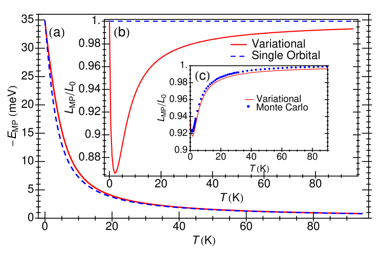
Figure 12: (Color online) (a) $T$-dependence of the MP energy [Eq. (49)] with the variationally-obtained (“renormalized”) (red/solid) and the fixed wave function for a harmonic QD confinement without Mn spins. (b) The corresponding $T$-dependence of the most probable width for a renormalized wave function, $L_{\text{MP}}$ (red/solid) and fixed wave function (blue/dashed), $L_{\text{MP}}\equiv L_{0}$, from Eq. (47). (c) $T$-dependence of the $L_{\text{MP}}$ from a variational method (red/solid) and Monte Carlo simulations (blue/dotted).

From Fig. 12(b) we see that the wave function renormalization itself is a small effect. The red/solid curve shows how the wave function width, normalized to the nonmagnetic width, $L_{0}$, varies with $T$. As the $T$ increases from $T=0$ K, the Mn spins coupled to the tail of the wave function are more prone to thermal excitation. The wave function shrinks to attain a more energetically favorable configuration by increasing the exchange energy gain from the polarized Mn spins near the center of the QD. Eventually, thermal excitation overcomes the magnetic energy, and the system relaxes continuously to a nonmagnetic state resulting in $L_{\text{MP}}=L_{0}$ at large $T$, as there is no energy gain from the wave function renormalization. From the variational approach we see an additional MP localization: $L_{\text{MP}}\leq L_{0}$, while the nonmonotonic $L_{\text{MP}}(T)$ implies also a nonmonotonic effective exchange fieldYakovlev:2010 due to the MP formation.

To further verify the renormalization effect of the MP wave function, we implement Monte Carlo simulations, removing the need of a variational calculations of the wave function. To approximate the MP wave function we include $s$, $p$, and $d$ orbitals in our simulation and allow for mixing of these orbitals. In Fig. 12(c) we see that both variational (red/solid) and Monte Carlo (blue/dotted) results agree well with each other and shown again a nonmonotonic $L_{\text{MP}}(T)$, noted also in Fig. 12(b). The slightly smaller wave function renormalization in Fig. 12(c), as compared to that in Fig. 12(b), is a consequence of fewer Mn spins in the middle region of the QD.

Appendix C Monte Carlo Simulations

Monte Carlo simulations were used to approximate solutions to the Schrödinger equation

$$\hat{H}(\{S\})\ket{\Phi}=E(\{S\})\ket{\Phi},$$ (50)

for a fixed finite orthonormal basis $\ket{\Phi}$ at a given Mn spin $(\{S\})$ configuration. The calculation entails guessing a Mn configuration at a given $T$, producing a matrix representation of $\hat{H}(\{S\})$ in a finite basis, and solving the eigenvalue problem.

The calculation begins by defining a 2D harmonic QD and solve for single heavy hole QD levels and eigenfunctions without any Mn atoms. We truncate the states up to the first $N$-orbitals. We obtain $N$ noninteracting wave functions $\phi_{n\sigma}^{0}({\bf r})$ at energy $E_{n}^{0}$ with $\sigma=\uparrow,\downarrow$. For a given configuration of $N_{\text{Mn}}$ Mn spins, {$S_{z1},S_{z2},...,S_{zN_{\text{Mn}}}$}, we construct a $(2N)\times(2N)$ matrix,

$$\hat{H}=\sum_{n\sigma}E_{n}^{0}\ket{\phi_{n\sigma}^{0}}\bra{\phi_{n\sigma}^{0}}+\sum_{nn^{\prime},\sigma}g_{nn^{\prime}\sigma}(\{S_{z}\})\ket{\phi_{n^{\prime}\sigma}^{0}}\bra{\phi_{n\sigma}^{0}}.$$ (51)

The interaction constant $g$ is

$$g_{nn^{\prime}\sigma}(\{S_{z}\})=\frac{\beta}{3}\sum_{j=1}^{N_{\text{Mn}}}[\phi_{n^{\prime}\sigma}^{0}({\bf R}_{j})]^{*}\left(s_{z,\sigma}S_{zj}\right)\phi_{n\sigma}^{0}({\bf R}_{j}),$$ (52)

where $s_{z}$ is the spin of the carrier and ${\bf R}_{j}$ is the position of the Mn ion. We diagonalize the single heavy hole Hamiltonian at a snapshot of $\{S_{z}\}$ and obtain eigenvalues $E_{i}(\{S_{z}\})$ and eigenvectors $c_{i,n\sigma}(\{S_{z}\})$. We then propose a different Mn-configuration, {$S^{\prime}_{z1},S^{\prime}_{z2},...,S^{\prime}_{zN_{\text{Mn}}}$}, diagonalize $\hat{H}(\{S^{\prime}_{z}\})$ and obtain new eigenvalues $E^{\prime}_{i}(\{S^{\prime}_{z}\})$.

References

- (1) E. M. Chudnovsky and L. Gunther, Phys. Rev. Lett. 60, 661 (1988).
- (2) J. R Friedman, M. P. Sarachik, J. Tejada, and R. Ziolo, Phys. Rev. Lett. 76, 3830 (1996).
- (3) D. A. Garanin and E. M. Chudnovsky, Phys. Rev. B 56, 11102 (1997).
- (4) J. Seufert, G. Bacher, M. Scheibner, A. Forchel, S. Lee, M. Dobrowolska, and J. K. Furdyna, Phys. Rev. Lett. 88, 027402 (2001).
- (5) R. Beaulac, L. Schneider, P. I. Archer, G. Bacher, and D. R. Gamelin, Science 325, 973 (2009).
- (6) J. Fernández-Rossier and R. Aguado, Phys. Rev. Lett. 98, 106805 (2007).
- (7) R. M. Abolfath, A. G. Petukhov, and I. Žutić, Phys. Rev. Lett. 101, 207202 (2008).
- (8) R. M. Abolfath, P. Hawrylak, and I. Žutić, Phys. Rev. Lett. 98, 207203 (2007).
- (9) R. Oszwaldowski, P. Stano, A.G. Petukhov, and I. Žutić, Phys. Rev. B 86, 201408(R) (2012).
- (10) R. Wasner (Ed.) Nanoelectronics and Information Technology 3 Edition (Wiley, Hoboken, 2012).
- (11) K. V. Raman, A. M. Kamerbeek, A. Mukherjee, N. Atodiresei, T. K. Sen, P. Lazić, V. Caciuc, R. Michel, D. Stalke, S. K. Mandal, S. Mandal, S. Blugel, M. Munzenberg, J. S. Moodera Nature 493, 509 (2013).
- (12) J.-Y. Chen, T.-M. Wong, C.-W. Chang, C.-Y. Dong, and Y.-F. Chen, Nat. Nanotech. 9, 845 (2014).
- (13) I. Žutić and P. E. Faria Junior, Nat. Nanotech. 9, 750 (2014).
- (14) D. D. DiVincenzo, Science 279, 255 (1995).
- (15) S. Thiele, F. Balestro, S. Klyatskaya, M. Ruben, W. Wernsdorfer, Science 344, 1135 (2014).
- (16) A. A. Maksimov, G. Bacher, A. McDonald, V. D. Kulakovskii, A. Forchel, C. R. Becker, G. Landwehr, and L. W. Molenkamp, Phys. Rev. B 62, R7767 (2000).
- (17) P. S. Dorozhkin, A. V. Chernenko, V. D. Kulakovskii, A. S. Brichkin, A. A. Maksimov, H. Schoemig, G. Bacher, A. Forchel, S. Lee, M. Dobrowolska, and J. K. Furdyna, Phys. Rev. B 68, 195313 (2003).
- (18) M. Holub, S. Chakrabarti, S. Fathpourand, P. Bhattacharya, Y. Lei, and S. Ghosh, Appl. Phys. Lett. 85, 973 (2004).
- (19) L. Besombes, Y. Leger, L. Maingault, D. Ferrand, H. Mariette, and J. Cibert, Phys. Rev. Lett. 93, 207403 (2004).
- (20) A. Hundt, J. Puls, A. V. Akimov, Y. H. Fan, and F. Henneberger, Phys. Rev. B 72, 033304 (2005).
- (21) T. Gurung, S. Mackowski, G. Karczewski, H. E. Jackson, and L. M. Smith, Appl. Phys. Lett. 93, 153114 (2008).
- (22) D. M. Hoffman, B. K. Meyer, A. I. Ekimov, I. A. Merkulov, Al. L. Efros, M. Rosen, G. Couino, T. Gacoin, and J. P. Boilot, Solid State Commun. 114, 547 (2000).
- (23) D. J. Norris, N. Yao, F. T. Charnock, and T. A. Kennedy, Nano Lett. 1, 3 (2001).
- (24) P. V. Radovanovic and D. R. Gamelin, J. Am. Chem. Soc. 123, 12207( 2001).
- (25) S. T. Ochsenbein, Y. Feng, K. M. Whitaker, E. Badaeva, W. K Liu, X. Li, and D. R. Gamelin, Nat. Nanotech. 4, 68 (2009).
- (26) I. Žutić and A. G. Petukhov, Nat. Nanotech. 4, 623 (2009).
- (27) D. A. Bussian, S. A. Crooker, M. Yin, M. Brynda, A. L. Efros, and V. I. Klimov, Nat. Mater. 8, 35 (2009).
- (28) R. Viswanatha, J. M. Pietryga, V. I. Klimov, and S. A. Crooker, Phys. Rev. Lett. 107, 067402 (2011).
- (29) R. Beaulac, Y. Feng, J. W. May, E. Badaeva, D. R. Gamelin, X. Li., Phys. Rev. B 84, 195324 (2011).
- (30) A. Pandey, S. Brovelli, R. Viswanatha, L. Li, J. M. Pietryga, V. I. Klimov, and S. A. Crooker, Nat. Nanotech. 7 , 792 (2012).
- (31) S. S. Farvid, T. Sabergharesou, L. N. Huffluss, M. Hegde, E. Prouzet, and P. V. Radovanovic, J. Am. Chem. Soc. 136, 7669 (2014).
- (32) B. Peng, J. W. May, D. R. Gamelin, and X. Li, J. Phys. Chem. 118, 7630 (2014).
- (33) F. Xiu, Y. Wang, J. Kim, P. Upadhyaya, Yi Zhou, X. Kou, W. Han, R. K. Kawakami, J. Zou, and K. L. Wang. ACS Nano 4, 4948 (2010).
- (34) I. R. Sellers, R. Oszwałdowski, V. R. Whiteside, M. Eginligil, A. Petrou, I. Žutić, W.-C. Chou, W. C. Fan, A. G. Petukhov, S. J. Kim, A. N. Cartwright, and B. D. McCombe, Phys. Rev. B 82, 195320 (2010);
- (35) B. Barman, R. Oszwałdowski, L. Schweidenback, A. H. Russ, J. M. Pientka, Y. Tsai, W-C. Chou, W. C. Fan, J. R. Murphy, A. N. Cartwright, I. R. Sellers, A. G. Petukhov, I. Žutić, B. D. McCombe, and A. Petrou, Phys. Rev. 92, 035430 (2015).
- (36) F. Henneberger and J. Puls, in Introduction to the Physics of Diluted Magnetic Semiconductors edited by J. Kossut and J. A. Gaj (Springer, Berlin, 2010).
- (37) Ł. Kłopotowski, Ł. Cywiński, P. Wojnar, V. Voliotis, K. Fronc, T. Kazimierczuk, A. Golnik, M. Ravaro, R. Grousson, G. Karczewski, and T. Wojtowicz, Phys. Rev. B 83, 081306(R) (2011).
- (38) Ł. Kłopotowski, Ł. Cywiński, M. Szymura, V. Voliotis, R. Grousson, P. Wojnar, K. Fronc, T. Kazimierczuk, A. Golnik, G. Karczewski, and T. Wojtowicz, Phys. Rev. B 87, 245316 (2013).
- (39) W. Pacuski,T. Jakubczyk, C. Kruse, J. Kobak, T. Kazimierczuk, M. Goryca, A. Golnik, P. Kossacki, M. Wiater, P. Wojnar, G. Karczewski, T. Wojtowicz, and D. Hommel, Cryst. Growth Des. 14, 998 (2014).
- (40) A. Kudelski, A. Lema tre, A. Miard, P. Voisin, T. C. M. Graham, R. J. Warburton, and O. Krebs, Phys. Rev. Lett. 99, 247209 (2007)
- (41) J. van Bree, P. M. Koenraad, and J. Fernandez-Rossier, Phys. Rev. B 78, 165414 (2008).
- (42) A. O. Govorov, Phys. Rev. B 70, 035321 (2004).
- (43) D. R. Yakovlev and W.Ossau, in Introduction to the Physics of Diluted Magnetic Semiconductors edited by J. Kossut and J. A. Gaj (Springer, Berlin, 2010).
- (44) T. Dietl and J. Spałek, Phys. Rev. Lett. 48, 355 (1982); T. Dietl and J. Spałek, Phys. Rev. B 28, 1548 (1983).
- (45) P. A. Wolff, in Semiconductors and Semimetals edited by J. K. Furdyna and J. Kossut (Academic Press, San Diego 1988), Vol. 25.
- (46) A. C. Durst, R. N. Bhatt, and P. A. Wolff, Phys. Rev. B 65, 235205 (2002).
- (47) J. K. Furdyna, J. Appl. Phys. 64 R29 (1988).
- (48) E. L. Nagaev, Physics of Magnetic Semiconductors (MIR Publishers, Moscow 1983).
- (49) T. Kasuya and A. Yanase, Rev. Mod. Phys. 40, 684 (1968).
- (50) T. Dietl, P. Peyla, W. Grieshaber, and Y. Merle d’ Aubigné, Phys. Rev. Lett. 74, 474 (1995).
- (51) D. D. Awschalom, J. Warnock, and S. von Molnár, Phys. Rev. Lett. 58, 812 (1987).
- (52) M. P. Marder Condensed Matter Physics 2 Edition (Wiley, Hoboken, 2010).
- (53) Clearly nanomagnets are finite and thus spatially-inhomogeneous systems which require using free energy functional or a closely related effective Hamiltonian [Ref. Dietl1982:PRL, ], not a spatially-independent MFA free energy, . However, we explain that a careful choice of the order parameter in can yield important trends in nanomagnets.
- (54) For a carrier-mediated magnetism in QDs this description would break down above for which the thermal energy exceeds the confinement energy leading to no carriers.
- (55) A. O. Govorov, Phys. Rev. B. 72, 075359 (2005).
- (56) A. O. Govorov, C. R. Physique 9, 857 (2008).
- (57) S.-J. Cheng, Phys. Rev. B. 77, 115310 (2008).
- (58) R. Oszwałdowski, I. Žutić, and A. G. Petukhov, Phys. Rev. Lett. 106, 177201 (2011).
- (59) H. Bednarski and J. Spałek, J. Phys.: Condens. Matter 24, 235801 (2012).
- (60) R. M. Abolfath, M. Korkusinski, T. Brabec, and P. Hawrylak Phys. Rev. Lett. 108, 247203 (2012).
- (61) I. L. Kuskovsky, W. MacDonald, A. O. Govorov, L. Mourokh, X. Wei, M. C. Tamargo, M. Tadic, and F. M. Peeters, Phys. Rev. B 76, 035342 (2007).
- (62) A. V. Chernenko, A. S. Brichkin, S. V. Sokolov, and S. V. Ivanov, Phys. Status Solidi B 247, 1514 (2010).
- (63) C. Gould, A. Slobodskyy, D. Supp, T. Slobodskyy, P. Grabs, P. Hawrylak, F. Qu, G. Schmidt, and L. W. Molenkamp, Phys. Rev. Lett. 97, 017202 (2006).
- (64) K. Matsuda, S. V. Nair, H. E. Ruda, Y. Sugimoto, T. Saiki, and K. Yamaguchi, Appl. Phys. Lett. 90, 013101 (2007).
- (65) B. Bansal, S. Godefroo, M. Hayne, G. Medeiros-Ribeiro, and V. V. Moshchalkov, Phys. Rev. B 80, 205317 (2009).
- (66) B. Fisher, J. M. Caruge, D. Zehnder, and M. Bawendi, Phys. Rev. Lett. 94, 087403 (2005).
- (67) L. Besombes, Y. Leger, L. Maingault, D. Ferrand, H. Mariette, and J. Cibert, Phys. Rev. B 71, 161307(R) (2005).
- (68) A. H. Trojnar, M. Korkusinski, U. C. Mendes, M. Goryca, M. Koperski, T. Smolenski, P. Kossacki, P. Wojnar, and P. Hawrylak, Phys. Rev. B 87, 205311 (2013).
- (69) S. Das Sarma, E. H. Hwang, and A. Kaminski Phys. Rev. B 67, 155201 (2003).
- (70) A. G. Petukhov, I. Žutić, and S. C. Erwin, Phys. Rev. Lett. 99, 257202 (2007).
- (71) J. M. Pientka, R. Oszwałdowski, A. G. Petukhov, J. E. Han and I. Žutić Phys. Rev. B 86, 161403(R) (2012).
- (72) J. Fernández-Rossier and L. Brey, Phys. Rev. Lett. 93, 117201 (2004).
- (73) N. Lebedeva, A. Varpula, S. Novikov, and P. Kuivalainen, Phys. Rev. B 81, 235307 (2010).
- (74) N. Lebedeva, A. Varpula, S. Novikov, and P. Kuivalainen, Phys. Status Solidi B 249, 2244 (2012).
- (75) D.P. Landau, K. Binder A Guide to Monte Carlo Simulations in Statistical Physics 3rd Edition (Cambridge University Press,Cambridge, 2009).
- (76) J. Lee, K. Vyborny, J. E. Han, and I. Žutić, Phys. Rev. B 89, 045315 (2014)
- (77) P. Stano, J. Fabian, and I. Žutić, Phys. Rev. B 87, 165303 (2013).
- (78) K. Vyborny, J. E. Han, R. Oszwałdowski, I. Žutić, and A. G. Petukhov, Phys. Rev. B 85, 155312 (2012).
- (79) C. Le Gall, A. Brunetti, H. Boukari, and L. Besombes Phys. Rev. Lett. 107, 057401 (2011).
- (80) P. Kłosowski, T. M. Giebułtowicz, J. J. Rhyne, N. Samarth, H. Luo, and J. K. Furdyna, J. Appl. Phys. 70, 6221 (1991).
- (81) By defnition, the open-shell systems have more of either “spin-up” or “spin-down” carriers.
- (82) R. Kubo, Statistical Mechanics (North-Holland, Amsterdam, 1960).
- (83) A. Golnik, J. Ginter, and J. A. Gaj, J. Phys. C 16, 6073 (1983).
- (84) C. Yannouleas and U. Landman, Rep. Prog. Phys. 70, 2067 (2007).
- (85) A. Ghosal, A. D. Guclu, C. J. Umrigar, D. Ullmo, and H. U. Baranger, Nat. Phys. 2, 336 (2006).
- (86) R. Egger, W. Häusler, C. H. Mak, and H. Grabert, Phys. Rev. Lett. 82, 3320 (1999).
- (87) C. Ellenberger, T. Ihn, C. Yannouleas, U. Landman, K. Ensslin, D. Driscoll, and A. C. Gossard, Phys. Rev. Lett. 96, 126806 (2006).
- (88) A. Singha, V. Pellegrini, A. Pinczuk, L. N. Pfeiffer, K. W. West, and M. Rontani, Phys. Rev. Lett. 104, 246802 (2010).
- (89) G. J. Schinner, J. Repp, E. Schubert, A. K. Rai, D. Reuter, A. D. Wieck, A. O. Govorov, A. W. Holleitner, and J. P. Kotthaus, Phys. Rev. Lett. 110, 127403 (2013).
- (90) This is a very accurate assumption for relatively small Mn content we consider here. The triplet state becomes relevant for a higher Mn content.Oszwaldowski2012:PRB
- (91) Even electric-field-induced redistribution of carriers could yield striking changes in magnetic ordering. For example, Ref. Abolfath2008:PRL, ; E. Dias Cabral, M. A. Boselli, R. Oszwałdowski, I. Žutić, and I. C. da Cunha Lima, Phys. Rev. B 84, 085315 (2011); L. D. Anh, P. N. Hai, Y. Kasahara, Y. Iwasa, and M. Tanaka, arXiv:1503.02174, preprint.
- (92) K. Zhao, Z. Deng, X. C. Wang, W. Han, J. L. Zhu, X. Li, Q. Q. Liu, R. C. Yu, T. Goko, B. Frandsen, L. Liu, F. Ning, Y. J. Uemura, H. Dabkowska, G. M. Luke, H. Luetkens, E. Morenzoni, S. R. Dunsiger, A. Senyshyn, P. Böni, and C. Q. Jin, Nat. Commun. 4, 1442 (2013).
- (93) K. Zhao, B. Chen, G. Zhao, Z. Yuan, Q. Liu, Z. Deng, J. Zhu, and C. Jin, Chin. Sci. Bull. 59, 2524 (2014).
- (94) J. K. Glasbrenner, I. Žutić, and I. I. Mazin, Phys. Rev. B 90, 140403(R) (2014).