Abstract

We introduce a minimal model for a collection of self-propelled apolar active particles, also called as ‘active nematic’, on a two-dimensional substrate and study the order-disorder transition with the variation of density. The particles interact with their neighbours within the framework of the Lebwohl-Lasher model and move asymmetrically, along their orientation, to unoccupied nearest neighbour lattice sites. At a density lower than the equilibrium isotropic-nematic transition density, the active nematic shows a first order transition from the isotropic state to a banded state. The banded state extends over a range of density, and the scalar order parameter of the system shows a plateau like behaviour, similar to that of the magnetic systems. In the large density limit the active nematic shows a bistable behaviour between a homogeneous ordered state with global ordering and an inhomogeneous mixed state with local ordering. The study of the above phases with density variation is scant and gives significant insight of complex behaviours of many biological systems.

Introduction :— Active systems are composed of self-propelled particles where each particle extracts energy from its surroundings and dissipates it through motion towards a direction determined by its orientation. These kind of systems are ubiquitous in nature, ranging from very small scale systems inside the cell to larger scales harada ; nedelec ; rauch ; benjacob ; animalgroups ; helbing ; feder ; kuusela31 ; hubbard , vibrated granular media vnarayan ; kudrolli etc., and have been studied extensively through experiments, theories and simulations sriramrmp ; tonertusr ; rev . A collection of head-tail symmetric ‘apolar’ active particles with an average mutual parallel alignment is said to be in a ‘nematic’ state, whereas in an ‘isotropic’ state particles remain randomly oriented. An active system where fluid media do not play important role in emergence of ordered state, and thus the hydrodynamic interactions can be ignored, is called a ‘dry active system’ kemkemer ; vnarayan ; animalgroups ; serra ; schaller ; surrey .

Active nature of particles introduces a nonequilibrium coupling between density and orientation field, as represented in terms of curvature coupling current in literature sradititoner ; shradhanjop ; sriramrmp . Such coupling in active nematic induces unusual properties like large density fluctuation sradititoner ; chateprl2006 and growth kinetics faster than $1/3$ as in usual conserved model shradhatrans2014 . Recent studies of the active nematic found a defect-ordered nematic state aparnaredner ; shimanatcomm ; yeomans as opposed to the equilibrium nematic for high particle densities. Recent experiment on amolyiod flibrils ncommam also found a phase with coexisting aligned and disordered fibril domains, similar to the defect-ordered state obtained in simulations. But few investigations have been done on the behaviours of the active nematic in various density limits, especially at low densities. Here we introduce a minimal model for two-dimensional active nematic and compare various ordering phases of active and equilibrium nematic in different density limits. The ordering in the system is characterised in terms of a scalar order parameter $S$ which is the positive eigen value of nematic order parameter Q pgdgenne in two-dimensions. In the low density limit both active and equilibrium systems are in the isotropic (I) state with particles randomly oriented throughout the whole system (see Fig. 1(b) - I), resulting in a small $S$. The Phase diagram of the active nematic as a function of packing density $C$ (see Fig. 1(a)) shows a jump in $S$ close to $C=0.37$, whereas in the equilibrium case $S$ goes continuously to larger values and an isotropic to nematic (I-N) transition occurs close to $C=0.58$. In the equilibrium nematic (EN) state particles remain homogeneously oriented in the system (see Fig. 1(b) - EN). At $C=0.37$ the active system goes from the isotropic to a banded state (BS) where particles cluster and align in the perpendicular direction to the long axis of the band (see Fig. 1(b) - BS-1). With increasing density more number of particles participate in band formation (see Fig. 1(b) - BS-2) and $S$ follows a plateau over a range of density. In the large density limit active system shows bistability between a homogeneous ordered (HO) (see Fig. 1(b) - HO) and an inhomogeneous mixed (IM) or local ordered state (see Fig. 1(b) - IM). This IM state is very similar to defect-ordered nematic state in ref. aparnaredner ; shimanatcomm ; yeomans .

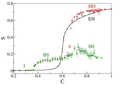
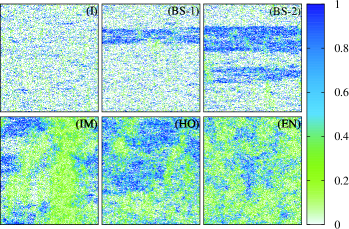
Figure 1: (Color online) (a) Plot of scalar order parameter $S$ vs. packing density $C$ for active (circles and triangles) and equilibrium (continuous line) nematic for system size $512$ $\times$ $512$. Equilibrium system goes smoothly from isotropic (I) to nematic (EN) state. Active system goes from isotropic (I) to banded state (BS) (small jump in $S$) followed by either an inhomogeneous mixed (IM) (triangles) or a homogeneous ordered (HO) (circles) state. (b) Snapshots of particle inclination towards the horizontal direction. Color bar ranging from zero to one indicates parallel and perpendicular inclinations respectively towards the horizontal direction. White regions signify unoccupied sites. (I) is isotropic state at low density ($C=0.36$), (BS-1) ($C=0.38$) and (BS-2) ($C=0.56$) are two banded state configurations, (IM) is inhomogeneous mixed, (HO) is homogeneous ordered and (EN) is equilibrium nematic state at high density ($C=0.76$).

Model :— We consider a two dimensional square lattice. At each vertex ‘$i$’ we define an occupation variable $n_{i}$, which can take values $1$ (occupied) or $0$ (unoccupied), and an orientation variable $\theta_{i}$, which lies between $0$ and $\pi$ because of the apolar nature of the particles. Each particle interacts with its nearest neighbours through modified Lebwohl - Lasher Hamiltonian llasher

$$\mathcal{H}=-\epsilon\sum_{<ij>}n_{i}n_{j}\cos 2(\theta_{i}-\theta_{j})$$ (1)

where $\epsilon$ is the interaction strength between two neighbouring particles. This model is analogous to the diluted XY-model with nonmagnetic impurities dilutedxymodel , where impurities and spins are analogous to vacancies and particles respectively in the present model.

Orientation evolves through Monte - Carlo (MC) updates mcbinder following the Hamiltonian in Eq. 1. Unlike the diluted XY-model, particles also move on the lattice. Depending on the type of movement we define two kinds of models. (i) ‘Equilibrium model’ (EM) - a particle can diffuse to any unoccupied nearest-neighbouring site, and therefore satisfies the detailed balance condition. (ii) ‘Active model’ (AM) - a particle can move to only those unoccupied nearest-neighbouring sites which are in the direction that makes the least inclination with the particle orientation. Details of the model and particle movement are shown in Supplemental Material SM section I. The asymmetric move of the active particles does not staisfy the detailed balance condition and arises in general because of the self-propelled nature of the particles in many biological kemkemer ; paxton and granular systems vnarayan . These moves produce an active curvature coupling current in coarse-grained hydrodynamic equations of motion shradhanjop ; sradititoner .

Numerical details :— We consider a collection of $N$ particles with random orientation $\theta_{i}\in[0,\pi]$, homogeneously distributed on a $L\times L$ square lattice ($L=150,256,512$) with periodic boundary condition. The packing density of the system is $C=N/(L\times L)$. We choose a particle randomly and move it to an unoccupied neighbouring site, followed by an orientation updation through MC. We use $10^{6}$ MC steps to evolve the system to its steady state and all the results have been obtained by averaging over next $2\times 10^{6}$ MC steps. Twenty four realizations have been used for better statistics.

We calculate the scalar order parameter

$$S=\sqrt{(\frac{1}{N}\sum_{i}n_{i}\cos(2\theta_{i}))^{2}+(\frac{1}{N}\sum_{i}n_{i}\sin(2\theta_{i}))^{2}}$$ (2)

which is small in the isotropic state and close to $1$ in the ordered state. First we calculate $S$ for EM as a function of inverse temperature $\beta=1/k_{B}T$ for different densities. As shown in Supplemental Material SM section II, the critical temperature $T_{c}$ is approximated as $T_{c}(S=0.4)$. Critical temperature $T_{c}(C)$ decreases with the lowering of the packing density $C$ , similar trend is found in the study of diluted XY-model dilutedxymodel for varying nonmagnetic site density. In rest of our calculations temperature is kept fixed at $\beta\epsilon=2.0$ and packing density $C$ is varied from small values to complete filling $C=1.0$.

Phase diagram :— At low densities, $C<0.37$, the active system is in the isotropic state where the particles with random orientation remain homogeneously distributed throughout the system, and therefore $S$ holds vanishingly small values. The jump occurs in $S$ at $C=0.37$. For $C\geq 0.37$ particles cluster in, and both ordered state with high local density and disordered state with low local density coexist (see Fig. 1(b) - BS-1). Mean alignment inside the band is perpendicular to the long axis of the band. In the moderate density limits, band formation in more favourable than lane formation (mean alignment parallel to the long axis of the structure) because the number of particles that can have translational motion is much larger in the banded state, and therefore entropy favours band formation. Similar mechanism create the bending instability close to order-disorder transition in the active polar systems chate ; shradhapre . The above transition from I state to BS occurs at density lower than the corresponding equilibrium I-N transition density $C\simeq 0.58$ (see Fig. 1(a)).

As we further increase $C$, unlike the equilibrium system where $S$ increases monotonically with $C$, the active system shows very small change in $S$ for a range of density. This plateau like appearance of $S$ with variation in $C$ is very similar to plateau phase in magnetization versus field curve of magnetic systems plateauphase . If an energy gap exists between two consecutive magnetic states, a finite field is required for the magnetic system to go from the lower to the higher state. So until that finite field is applied, the increasing field keeps the system magnetization to be unchanged, and the system is called to be in the plateau phase. With increasing packing density in the plateau regime of the active nematic more particles participate in band formation (see Fig. 1(b) - BS-1 and BS-2). On further increment of density, close to equilibrium I-N transition $C\simeq 0.58$, transverse fluctuations lead the system to a mixed state shradhanjop ; shimaprl2011 .

In the large $C$ limit active system shows a bistable behaviour with two distinct steady states; first, a state where $S$ is large and real space configuration is ‘homogeneous ordered’ (HO), and the second, an ‘inhomogeneous mixed’ (IM) state where $S$ realizes some moderate values. In the HO state though the particle orientation is homogeneous, large density inhomogeneity exists in the system (see Fig. 1(b) - HO). IM state is a local ordered state with many aligned clusters of high particle density. The system consists of many such aligned clusters of high density separated from low density disordered regions and mean alignment in each cluster is in different directions (see Fig. 1(b) - IM). IM state is similar to the defect-ordered state recently found in the study of ref. shimanatcomm ; aparnaredner ; yeomans , with large number of $\pm 1/2$ defects in high density active nematic.

Renormalised mean field study for small $S$:— We also calculate the jump in the scalar order parameter $S$ and the shift in the transition density using the Renormalised mean field (RMF) method of the coupled coarse-grained hydrodynamic equations of motion for the number density $\rho({\bf r},t)=\sum_{\alpha}\delta({\bf r}-{\bf R}_{\alpha}(t))$ and the order parameter ${\bf w}_{ij}({\bf r},t)=\rho({\bf r},t)\mbox{Q}({\bf r},t)=\sum_{\alpha}({\bf m}_{i\alpha}{\bf m}_{j\alpha}-\frac{1}{2}\delta_{ij})\delta({\bf r}-{\bf R}_{\alpha}(t))$ for active nematic shradhanjop ; sradititoner .

$$\partial_{t}\rho=a_{0}\nabla_{i}\nabla_{j}{\bf w}_{ij}+D_{\rho}\nabla^{2}\rho$$ (3)

and

$$\partial_{t}{\bf w}_{ij} =\left\{\alpha_{1}\left(\rho\right)-\alpha_{2}\left(\mathbf{w}:\mathbf{w}\right)\right\}{\bf w}_{ij}$$

$$+\beta\left(\nabla_{i}\nabla_{j}-\frac{1}{2}\delta_{ij}\nabla^{2}\right)\rho+D_{\bf w}\nabla^{2}{\bf w}_{ij}$$ (4)

where, ${\bf m}_{\alpha}=(\cos(\theta_{\alpha}),\sin(\theta_{\alpha}))$ is the unit vector along the orientation $\theta_{\alpha}$ and ${\bf R}_{\alpha}(t)$ is the position of particle $\alpha$. We can obtain the number density $\rho$ by coarse-graining $C$ over small subvolume. Eqs. 3 and 4 can be obtained either from symmetry arguments as in ref. sradititoner or from microscopic rule based model shradhanjop . Density equation 3 is a continuity equation $\partial_{t}\rho=-\nabla\cdot{\bf J}$, because the total number of particles is conserved. Current $J_{i}=-a_{0}\nabla_{j}{\bf w}_{ij}-D_{\rho}\nabla_{i}\rho$, where the first term consists of two parts, an active curvature coupling current ${\bf J}_{a}\propto a_{0}{\rho\nabla_{j}\mbox{Q}_{ij}}$ and anisotropic diffusion ${\bf J}_{p1}\propto\mbox{Q}_{ij}\nabla_{i}\rho$, which can also be present in the equilibrium model. The second term in density equation is an isotropic diffusion ${\bf J}_{p2}\propto\nabla\rho$ term. First two terms in the order parameter equation ${\bf w}_{ij}$ is the alignment term. We choose $\alpha_{1}(\rho)=(\frac{\rho}{\rho_{IN}}-1)$ as a function of density which changes sign at some critical density $\rho_{IN}$. Third term is coupling to density and last term is diffusion in order parameter and written for equal elastic constant approximation for two-dimensional nematic.

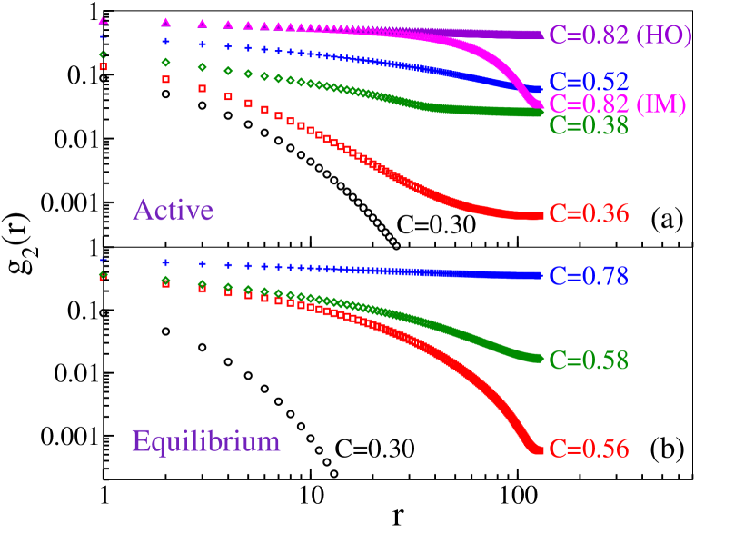
Figure 2: (Color online) $g_{2}(r)$ vs. $r$ on log-log scale at different densities. (a) Active nematic: ($\bigcirc$) and ($\square$) at low densities $g_{2}(r)$ decays exponentially, ($\diamond$) and ($+$) at intermediate density $g_{2}(r)$ decays algebraically, ($\bigtriangleup$) homogeneous ordered (algebraic decay), and inhomogeneous mixed (abrupt decay) at high density. (b) Equilibrium nematic ($\bigcirc$) and ($\square$) exponential decay of $g_{2}(r)$ at low densities and ($\diamond$) and ($+$) algebraic decay of $g_{2}(r)$ at high densities.

A homogeneous steady state solution of Eqs. 3 and 4 gives a mean field transition from isotropic to nematic state at density $\rho_{IN}$ where $\alpha_{1}(\rho)$ changes sign. Using RMF method we calculate the effective free energy $f_{eff}(S)$ close to order-disorder transition when $S$ is small. We consider density fluctuations $\delta\rho$ and neglect order parameter fluctuations. The effective free energy

$$f_{eff}\left(S\right)=-\frac{b_{2}}{2}S^{2}-\frac{b_{3}}{3}S^{3}+\frac{b_{4}}{4}S^{4}$$ (5)

where $b_{2}=\alpha_{1}(\rho)+\alpha_{1}^{\prime}(\rho)c$, where $c$ is a constant. $\alpha_{1}^{\prime}(\rho)={\partial\alpha_{1}/\partial\rho|}_{\rho_{0}}$, $b_{3}=\frac{a_{0}\alpha_{1}^{\prime}(\rho)}{2D_{\rho}}$ and $b_{4}=\frac{1}{2}\alpha_{2}$. Both $b_{3}$ and $b_{4}$ are positive. A detail calculation for $f_{eff}$ is shown in Supplemental Material SM section III. The density flcutuations introduce a new cubic order term protortional to the activity strength $a_{0}$, in the free energy $f_{eff}(S)$. The presence of such term produces a jump $\Delta S=S_{c}=\frac{2b_{3}}{3b_{4}}$ at a lower density $\rho_{c}=\rho_{IN}(1-\frac{2b_{3}^{2}}{9b_{4}})$. This type of jump and shift in transition because of flcutuations are also called as fluctuation dominated first order phase transition in statistical mechanics coleman and widely studied in many systems fdfopt . The jump in $S$ and the shift in $\rho_{c}$ is proportional to the activity parameter $a_{0}$ and for $a_{0}=0$ we recover the equilibrium transition.

Two-point orientation correlation function :— To further characterise the system we also calculate the two-point orientation correlation $g_{2}(r)=<\sum_{i}n_{i}n_{i+r}\cos[2\left(\theta_{i}-\theta_{i+r}\right)]/\sum_{i}n_{i}n_{i}>$ at different packing densities, where $<.>$ signifies an average over many realisations. In Fig. 2 we plot $g_{2}(r)$ vs. $r$ on log-log scale, for $C=0.30$, $0.36$, $0.38$, $0.52$ and $0.82$ for active model and $C=0.30$, $0.56$, $0.58$ and $0.78$ for equilibrium model. For very small packing density $C<0.37$, $g_{2}(r)$ decays exponentially in the active systems. Therefore the system is in short-range-ordered (SRO) isotropic state. At $C=0.38$, $g_{2}(r)$ decays following the power law $g_{2}(r)\simeq 1/r^{\eta(C)}$ and therefore the system is in a quasi-long-range-ordered (QLRO) state. At high packing densities correlation functions confirm the bistability in the active systems. For $C=0.82$ (see Fig. 2(a)) $g_{2}(r)$ shows power law decay in HO state, whereas in IM state $g_{2}(r)$ decays abruptly after a distance $r$. The abrupt change in $g_{2}(r)$ at a certain distance indicates the presence of local ordered clusters. In contrast, the equilibrium systems show a transition from SRO isotropic state at low density $C\>\raisebox{-2.15277pt}{$\stackrel{{\scriptstyle\textstyle<}}{{\sim}}$}\>0.56$ to QLRO nematic state at $C\>\raisebox{-2.15277pt}{$\stackrel{{\scriptstyle\textstyle>}}{{\sim}}$}\>0.58$, similar to Berezinskii - Kosterlitz - Thouless (BKT) transition Berezinskii ; KT in the diluted XY-model dilutedxymodel .

Orientation distribution :— We also compare the steady state properties of active and equilibrium models in the high density limit. First we calculate the steady state (static) orientation distribution $P(\theta)$ from one snapshot of particle orientation. Both active HO and equilibrium nematic show a Gaussian distribution of orientation (see Fig. 3(a)). Hence in HO state orientation fluctuations of particles are of same kind as in equilibrium model and the system is in QLRO state. Distribution $P(\theta)$ in the IM state is very broad and spanning the whole range of orientation. Hence the system has many local ordered regions with different orientations.

We also calculate the time averaged distribution of mean orientation of all the particles $P(\theta_{m})$ in active HO and equilibrium nematic states. $P(\theta_{m})$ is calculated from mean of all particle orientaions averaging over a long time (from $10^{6}$ to $3\times 10^{6}$) in the steady state. $P(\theta_{m})$ for HO is narrow in comparison to the broad distribution for equilibrium model (see Fig. 3(b)). Narrow distribution of $P(\theta_{m})$ implies that orientation autocorrelation in active system decay slowly as comapared to the corresponding equilibrium model which is in agreement with the slow decay of velocity autocorrelation in bacterial suspension wulib .

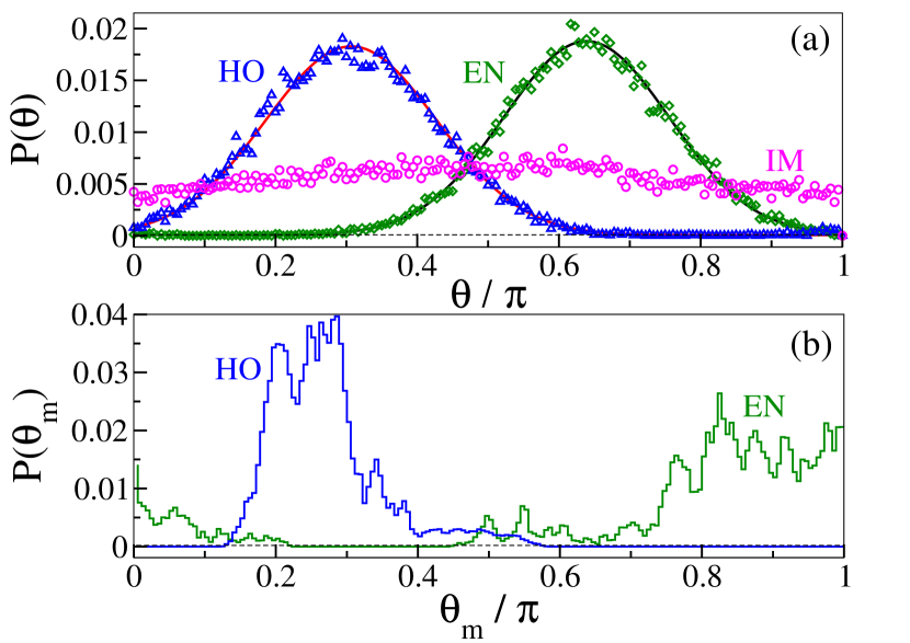
Figure 3: (Color online) (a) Steady state orientation distribution $P(\theta)$ of particles for HO, IM (active) and EN (equilibrium) states at high density. Lines are fit to Gaussian distribution for both HO and EN states. IM state shows very broad distribution of $P(\theta)$. (b) Plot of mean orientation distribution $P(\theta_{m})$ averaged over a long time in the steady state for HO (active) and EN (equilibrium) states. $P(\theta_{m})$ is very broad for EN in comparison to HO.

Summary :— In this letter we have introduced a minimal model for active nematic and found three distinct phases with the variation in density. At low densities the active nematic is in disordered isotropic state with very small correlation between the particles. With increasing density active nematic undergoes a fluctuation induced first order phase transition from the isotropic to the banded state where large number of particles participate in band formation. Large density fluctuations in the active systems change the nature of the transition and shift the transition density to smaller value as compared to the equilibrium isotropic nematic transition. At large densities equilibrium nematic is in QLRO nematic state, whereas active nematic goes from the banded state to either the homogeneous ordered (high $S$) or the inhomogeneous mixed (moderate $S$) state. This inhomogeneous mixed state is similar to the phase with coexisting aligned and disordered fibril domains found in recent experiment ncommam . Experiments on thin layer of agitated granular rods, elongated living cells, bacterial colony of apolar B. subtilis etc. at different densities can realize the different phases we found here. In the present model we have frozen the motion of the active particles in the transverse direction, i.e. the activity strength is kept large. It will be interesting to see the evolution of different phases with the particles having a small probability to move in transverse directions as well.

Supplemental Material

I I. Model figure

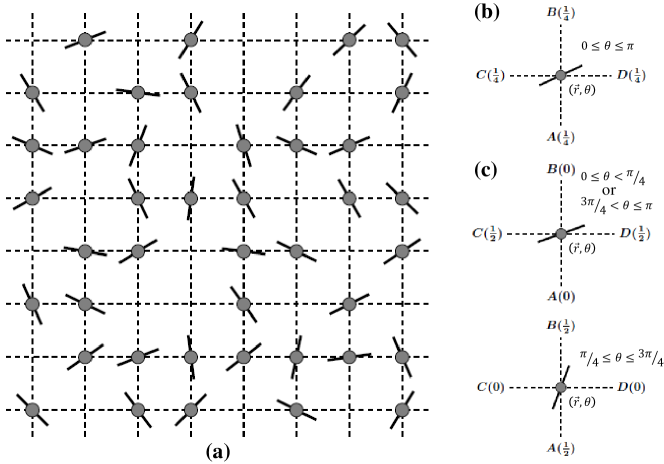
Figure 4: (a) Two dimensional square lattice with occupied ($n=1$) or unoccupied ($n=0$) sites. Filled circles signify the occupancy of respective sites. Inclination of the rods towards the horizontal direction show respective particle orientation $\theta_{i}\in\left[0,\pi\right]$. (b) Equilibrium move : particle can move to any of four neighbouring sites with equal probability $1/4$, (c) Active move: particle can move to either of its two neighbouring sites with probability $1/2$, if unoccupied, in the direction it is more inclined to.

II II. Estimate of critical temprature $T_{c}(C)$ in equilibrium model

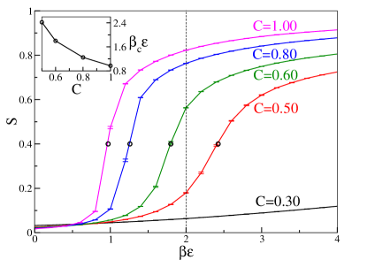
Figure 5: Plot of $S$ vs. inverse temperature $\beta\epsilon$ for different densities $C$ for equilibrium model. System goes from isotropic (small $S$) to nematic (large $S$) state. Vertical dotted line shows the variation in $S$ for fixed $\beta\epsilon=2.0$ at different densities. Crtical temperature is approximated as $T_{c}(S=0.4)$. Inset: change in $T_{c}$ as a function of density $C$.

III III. Renormalised mean field (RMF) study of active nematic for small scalar order parameter $S$

In this section we will write an effective renormalised mean field free energy for scalar order parameter $S$ for small $S$. We keep the density fluctuations and ignore the order parameter fluctuations in the coupled hydrodynamic equations of motion for active nematic. Density fluctuation produces a cubic order term in the effective free energy for scalar order parameter $S$ and such term produces a jump in $S$ at a new transition density $\rho_{c}$ lower than equilibrium I-N transition point $\rho_{IN}$. Shift in transition density and jump $\Delta S$ is directly proportional to the activity parameter $a_{0}$ and we recover equilibrium limit for zero $a_{0}$.
We write coupled hydrodynamic equations of motion for density $\rho$ and order parameter ${\bf w}=\rho\mbox{Q}$ where nematic order parameter pgdgenne

$$\mbox{Q}({\bf r},t)=S\left(\begin{array}[]{c c}\cos 2\theta({\bf r},t)&\sin 2\theta({\bf r},t)\\ \sin 2\theta({\bf r},t)&-\cos 2\theta({\bf r},t)\end{array}\right)$$ (8)

$\theta$ being the coarse grained angle at position ${\bf r}$ and time $t$. Density equation

$$\partial_{t}\rho=a_{0}\nabla_{i}\nabla_{j}{\bf w}_{ij}+D_{\rho}\nabla^{2}\rho$$ (9)

and order parameter equation ${\bf w}$

$$\partial_{t}{\bf w}_{ij}=\left\{\alpha_{1}\left(\rho\right)-\alpha_{2}\left(\bf{w}:\bf{w}\right)\right\}{\bf w}_{ij}+\beta\left(\nabla_{i}\nabla_{j}-\frac{1}{2}\delta_{ij}\nabla^{2}\right)\rho+D_{{\bf w}}\nabla^{2}{\bf w}_{ij}$$ (10)

Density Eq. 9 is a continuity equation $\partial\rho/\partial t=-\nabla\cdot{\bf J}$, where ${\bf J}$ has two parts, active and diffusive. Details of these two currents are given in the main text. $a_{0}$ is the activity parameter, present because of self-propelled nature of the particles, $\beta$ is the coupling of density in ${\bf w}$ equation. $D_{\rho}$ and $D_{\bf w}$ are the diffusion coefficients in density and order parameter equations respectively, $\alpha_{1}(\rho)$ and $\alpha_{2}$ are the alignment terms and ingeneral depends on the model parameters. For metric distance interacting models njopshradha $\alpha_{1}(\rho)$ is a function of density and changes sign at some critical density. We choose $\alpha_{1}(\rho)=\frac{\rho}{\rho_{IN}}-1$ and $\alpha_{2}=1$. Steady state solution of homogeneous Eq. 9 is $\rho=\rho_{0}$, we add small perturbation to mean density $\rho=\rho_{0}+\delta\rho$. In the staedy state density fluctuation $\delta\rho$ can be obtained from Eq. 9,

$$a_{0}\nabla_{i}\nabla_{j}{\bf w}_{ij}+D_{\rho}\nabla^{2}\delta\rho=0$$

$$\Rightarrow a_{0}\nabla_{j}{\bf w}_{ij}+D_{\rho}\nabla_{i}\delta\rho=constant=\mathbf{c_{1}}$$ (11)

where ${\bf w}_{11}=-{\bf w}_{22}=\frac{S}{2}\cos(2\theta)$ and ${\bf w}_{12}={\bf w}_{21}=\frac{S}{2}\sin(2\theta)$ and keep the lowest order terms in $S$ and $\theta$

$$\partial_{x}\delta\rho=-\frac{a_{0}}{D_{\rho}}\partial_{x}S\rightarrow\delta\rho(x)=-\frac{a_{0}}{D_{\rho}}S+c$$ (12)

and

$$\partial_{y}\delta\rho=\frac{a_{0}}{D_{\rho}}\partial_{y}S\rightarrow\delta\rho(y)=\frac{a_{0}}{D_{\rho}}S+c_{1}$$ (13)

Here we assume nematic is aligned along one direction and there is variation only along the perpendicular direction. Hence we can choose either of equations 12 or 13. Two constants $c$ and $c_{1}$ are the value of density where nematic order parameter is zero.

We use Eq. 12 and substitute the solution for density in equation for ${\bf w}_{ij}$ and obtain an effective equation for $S$.

$$\partial_{t}S=\left\{\alpha_{1}\left(\rho\right)-\frac{1}{2}\alpha_{2}S^{2}\right\}S+\mathcal{O}(\nabla^{2}S)+\mathcal{O}(\nabla^{2}\rho)$$ (14)

We neglect all the derivative terms and keep only polynomial in $S$, i.e. we neglect higher order fluctuations. We can do taylor expansion of $\alpha_{1}(\rho)$ about mean density $\rho_{0}$, $\alpha_{1}(\rho)=\alpha_{1}(\rho_{0}+\delta\rho)=\alpha_{1}(\rho_{0})+\alpha_{1}^{\prime}\delta\rho$, where $\alpha_{1}^{\prime}=\frac{\partial\alpha_{1}}{\partial\rho}|_{\rho_{0}}$. Substitute the expression for $\delta\rho$ from Eq. 12 hence

$$\partial_{t}S=\left\{\alpha_{1}\left(\rho_{0}\right)+\alpha_{1}^{\prime}\delta\rho-\frac{1}{2}\alpha_{2}S^{2}\right\}S$$ (15)

We can write an effective free energy for $S$

$$\partial_{t}{S}=-\frac{\delta f_{eff}(S)}{\delta S}$$ (16)

hence

$$-\frac{\delta f_{eff}}{\delta S}=S\left\{{\alpha_{1}\left(\rho_{0}\right)+\alpha}\left(\rho_{0}\right)\left(\frac{a_{0}}{2D_{\rho}}S+c_{1}\right)-\frac{1}{2}\alpha_{2}S^{2}\right\}$$ (17)

Therefore

$$f_{eff}\left(S\right)=-\frac{b_{2}}{2}S^{2}-\frac{b_{3}}{3}S^{3}+\frac{b_{4}}{4}S^{4}$$ (18)

where $b_{2}=\alpha_{1}\left(\rho_{0}\right)+\alpha_{1}^{\prime}c$, $b_{3}=\frac{a_{0}\alpha_{1}^{\prime}}{2D_{\rho}}$ and $b_{4}=\frac{1}{2}\alpha_{2}$ and $c$ is a conatant. Hence fluctuation in density introduces a cubic order term in effective free energy $f_{eff}(S)$. Effective free energy in Eq. 18 is similar to Landau free energy with cubic order term chaiklub . We calculate jump $\Delta S$ and new critical density from coexistence condition for free energy. Steady state solutions of order parameter ($S=0$ for isotropic and $S\neq 0$ for ordered state) are given by

$$\frac{\delta f_{eff}}{\delta S}=\left(-b_{2}-b_{3}S+b_{4}S^{2}\right)S=0$$ (19)

Non-zero $S$ is given by $-b_{2}-b_{3}S_{c}+b_{4}S_{c}^{2}=0$. Coexistence condition implies

$$f_{eff}(S_{c})=\left(-\frac{b_{2}}{2}-\frac{b_{3}}{3}S_{c}+\frac{b_{4}}{4}S_{c}^{2}\right)S_{c}^{2}=f_{eff}(S=0)=0$$ (20)

hence we get the solution

$$S_{c}=-\frac{3b_{2}}{b_{3}}$$ (21)

and

$$b_{2}^{c}=-\frac{2b_{3}^{2}}{9b_{4}}$$ (22)

Hence the jump at new critical point is $\Delta S=\frac{2b_{3}}{3b_{4}}$. Since $b_{4}>0$ and hence $b_{2}^{c}<0$, the new critical density

$$\rho_{c}=\rho_{IN}\left(1-\frac{2b_{3}^{2}}{9b_{4}}\right)<\rho_{IN}$$ (23)

is shifted to lower density in comparison to equilibrium $\rho_{IN}$. Eq. 23 gives the expression for new transition density as given in main text. Hence using renormalised mean field theory we find a jump $\Delta S$ at a lower density as compared to equilibrium I-N transition density.

References

- (1) P. G. de Gennes and J. Prost, The Physics of Liquid Crystals (Clarendon Press, Oxford, 1995).
- (2) E. Bertin, H. Chaté, F. Ginelli, S. Mishra, A. Peshkov and S. Ramaswamy, New J. of Phys. 15, 085032 (2013).
- (3) P. M. Chaikin and T. C. Lubensky, Principles of Condensed Matter Physics (Cambridge University Press, Cambridge, 2000).