$\alpha_{s}$ from the updated ALEPH data for hadronic $\tau$ decays

Abstract

We extract the strong coupling $\alpha_{s}(m_{\tau}^{2})$ from the recently updated ALEPH non-strange spectral functions obtained from hadronic $\tau$ decays. We apply a self-consistent analysis method, first tested in the analysis of OPAL data, to extract $\alpha_{s}(m_{\tau}^{2})$ and non-perturbative contributions. The analysis yields $\alpha_{s}^{\rm FO}(m_{\tau}^{2})=0.296\pm 0.010$, using Fixed Order Perturbation Theory (FOPT), and $\alpha^{\rm CI}_{s}(m_{\tau}^{2})=0.310\pm 0.014$, using Contour Improved Perturbation Theory (CIPT). The weighted average of these results with those previously obtained from OPAL data give $\alpha_{s}^{\rm FO}(m_{\tau}^{2})=0.303\pm 0.009$ and $\alpha_{s}^{\rm CI}(m_{\tau}^{2})=0.319\pm 0.012$, which gives, after evolution to the $Z$ boson mass scale, $\alpha^{\rm FO}_{s}(m_{Z}^{2})=0.1165\pm 0.0012$ and $\alpha_{s}^{\rm CI}(m_{Z}^{2})=0.1185\pm 0.0015$, respectively. We observe that non-perturbative effects limit the accuracy with which $\alpha_{s}$ can be extracted from $\tau$ decay data.

1 Introduction

The extraction of $\alpha_{s}$ from hadronic $\tau$ decays represents an important test of the evolution of the strong coupling as predicted by the QCD $\beta$-function. At and around the $\tau$ mass, $m_{\tau}\approx 1.78$ GeV, perturbative QCD can still be used, but realistic analyses must include the contribution from non-perturbative effects. The standard framework to describe hadronic $\tau$ decays is to organize the QCD description in an operator product expansion (OPE) where, apart from the perturbative contribution and quark-mass corrections, the QCD condensates intervene [1].

Observables such as $R_{\tau}$,

$$R_{\tau}=\frac{\Gamma\left[\tau^{-}\to\nu_{\tau}{\rm hadrons}(\gamma)\right]}{\Gamma\left[\tau^{-}\to\nu_{\tau}e^{-}\bar{\nu}_{e}(\gamma)\right]},$$ (1)

can be written as weighted integrals over the experimentally accessible QCD spectral functions. The spectral functions have been determined at LEP by the ALEPH [2] and OPAL collaborations [3]. In the specific case of $R_{\tau}$, the weight function is that determined by $\tau$-decay kinematics and the integral runs over the total energy of the hadronic system in the final state, $s$, from zero to $m_{\tau}^{2}$. Since the OPE description is not valid at low-energies the evaluation of the theoretical counterpart is performed exploiting the analytical properties of the QCD correlators. One writes then a finite-energy sum rule (FESR) where the theoretical counterpart of the observable is obtained from an integral along a complex circle of fixed radius $|s|=m_{\tau}^{2}$. In fact, any analytic weight function gives rise to a valid sum rule, and it has become customary to exploit this freedom in order to analyse several FESRs simultaneously. This type of combined analysis allows for the extraction of $\alpha_{s}$ as well as non-perturbative contributions.

The computation, in 2008, of the NNNLO term, $\mathcal{O}(\alpha_{s}^{4})$, of the perturbative expansion of the QCD correlators [4] triggered several reanalyses of $\alpha_{s}$ from $\tau$ decays [5, 6, 7, 8]. In the process, it was discovered that the correlation matrices of the then publicly available spectral functions from the ALEPH collaboration had a missing contribution from the unfolding procedure [9]. (It was for this reason that we restricted our attention to OPAL data in the analyses of Refs. [7, 8].) Recently, a new analysis of the ALEPH data became available, employing a new unfolding method, which corrects for this problem in the correlation matrices [10, 11]. The ALEPH spectral functions have smaller errors than OPAL’s and have the potential to constrain the theoretical description better. The new set of ALEPH spectral functions motivates the present reanalysis.

On the theoretical side, two different aspects have received attention recently. The first one regards the use of the renormalization group in improving the perturbative series. There are several prescriptions as to how one should set the renormalization scale. The most commonly used are Contour Improved Perturbation Theory (CIPT) [12] and Fixed Order Perturbation Theory (FOPT) [13]. Different prescriptions lead to different results with the available terms of the perturbative expansion, and therefore to different values of $\alpha_{s}$. This discrepancy remains one of the largest sources of uncertainty in $\alpha_{s}$ extractions from $\tau$ decays. Strong evidence in favour of the FOPT prescription has been given in Refs. [14, 15] but the issue is still under debate. Here, we chose to perform our analysis using both prescriptions and hence quote two values of $\alpha_{s}$.

The second point that has been studied recently is the description of non-perturbative effects. Since the work of Ref. [5] it is known that the OPE parameters obtained in some of the recent analyses are inconsistent. With these parameters one cannot account properly for the experimental results when $s_{0}$, the upper limit of the integration in the FESR, is lowered below $m_{\tau}^{2}$. A strategy that allows for a self-consistent analysis is the inclusion of Duality Violation (DV) effects in the theoretical description. It is well known that in the vicinity of the Minkowski axis the OPE alone cannot account for all non-perturbative effects. In the past, in the description of $R_{\tau}$, this contribution was systematically ignored due to the fortuitous double zero of the weight function at the Minkowski axis. In the same spirit, combined analyses of several FESRs were restricted to the so-called pinched moments, i.e., moments that have a zero at the the Minkowski axis. Until recently, DVs were not tackled directly and their contribution to final results and errors were not systematically assessed.

Recent progress in modeling the DV contribution [17, 18, 19, 20, 21] has allowed for analyses that include them explicitly in the FESRs. In Refs. [7] a new analysis method taking into account DVs explicitly was presented. This led to a determination of $\alpha_{s}$ from OPAL data in a self-consistent way, together with the OPE contribution and DV parameters [8]. In a recent work, we applied the same analysis method to the updated version of the ALEPH non-strange spectral functions [22].

In the remainder we discuss the main results of Ref. [22].

2 Analysis framework

For the sake of self-consistency, here we make a brief review of the framework of our analysis. The details can be found in the original publications Refs. [7, 8, 22].

Fits performed in our analysis are based on FESRs of the following form [16, 1]

$$I^{(w)}_{V/A}(s_{0}) \equiv \int_{0}^{s_{0}}\frac{ds}{s_{0}}\;w(s)\;\rho^{(1+0)}_{V/A}(s)$$ (2)

$$= -\frac{1}{2\pi i}\oint_{|s|=s_{0}}\frac{ds}{s_{0}}\;w(s)\;\Pi^{(1+0)}_{V/A}(s)\ ,$$

where the weight-functions $w(s)$ are polynomials in $s$, and $\Pi^{(1+0)}_{V/A}(s)$ is given by

$$i\int d^{4}x\,e^{iqx}\,\langle 0|T\left\{J_{\mu}(x)J_{\nu}^{\dagger}(0)\right\}|0\rangle$$

$$=\left(q_{\mu}q_{\nu}-q^{2}g_{\mu\nu}\right)\Pi^{(1+0)}(s)+q^{2}g_{\mu\nu}\Pi^{(0)}(s)\ ,$$ (3)

with $s=q^{2}=-Q^{2}$, and $J_{\mu}$ one of the non-strange $V$ or $A$ currents $\bar{u}\gamma_{\mu}d$ or $\bar{u}\gamma_{\mu}\gamma_{5}d$. The superscripts $(0)$ and $(1)$ refer to spin. In the sum rule Eq. (2), $\rho^{(1+0)}_{V/A}$ is the experimentally accessible spectral function. We construct FESRs at several values of $s_{0}\leq m_{\tau}^{2}$ for a given weight function.

The correlators $\Pi^{(1+0)}_{V/A}(s)$ can be decomposed exactly into three parts

$$\Pi^{(1+0)}(s)=\Pi^{(1+0)}_{\rm pert}(s)+\Pi^{(1+0)}_{\rm OPE}(s)+\Pi^{(1+0)}_{\rm DV}(s),$$ (4)

where “pert” denotes perturbative, “OPE” refers to OPE corrections of dimension larger than zero (including quark-mass corrections), and “DV” denotes the DV contributions to $\Pi^{(1+0)}(s)$.

It is convenient to write the perturbative contribution in terms of the physical Adler function [13, 14], that satisfies a homogeneous renormalization group equation. When treating the contour integration, one must adopt a prescription for the renormalization scale. As discussed above, we perform our analysis within CIPT and FOPT and quote both results.

The leading contributions from higher dimensions in the OPE can be parametrized with effective coefficients $C_{D}$ as

$$\Pi^{(1+0)}_{\rm OPE}(s)=\sum_{k=1}^{\infty}\frac{C_{2k}(s)}{(-s)^{k}}\ .$$ (5)

The dimension-two quark-mass corrections can safely be neglected for the non-strange correlators. Therefore, in our analysis $C_{2}=0$. The first non-negligible contribution is then $C_{4}$, that can be related to the gluon condensate. However, the weight functions employed in our analysis are polynomials constructed from combinations of the unity, $s^{2}$, and $s^{3}$. Therefore, in our FESRs, the leading contributions from the OPE arise solely from $C_{6}$ and $C_{8}$. We neglect subleading logarithmic corrections and treat all $C_{D}$ as constants.

The DV contribution to the sum rules can be written as

$${\cal D}_{w}(s_{0})=-\int_{s_{0}}^{\infty}\frac{ds}{s_{0}}\,w(s)\,\rho^{\rm DV}(s),$$ (6)

where $\rho^{\rm DV}(s)$ is the DV part of the spectral function in a given channel

$$\rho^{\rm DV}(s)=\frac{1}{\pi}\,\mbox{Im}\,\Pi^{(1+0)}_{\rm DV}(s),$$ (7)

that, for $s$ large enough, we parametrize with the Ansatz of Ref. [18, 19]

$$\rho^{\rm DV}_{V/A}(s)=\mbox{exp}\left(-\delta_{V/A}-\gamma_{V/A}s\right)\sin\left(\alpha_{V/A}+\beta_{V/A}s\right).$$ (8)

This adds 4 new parameters in each channel.

We do not restrict our analysis to pinched weight functions. Rather, we include a weight function that is not pinched in order to constrain the DV parameters better. We work with three weight functions, namely,

$$w_{1} = 1,$$

$$w_{2} = 1-x^{2},$$

$$w_{3} = (1-x^{2})(1+2x),$$ (9)

where $x\equiv s/s_{0}$. (The weight function $w_{3}$ is the one determined by kinematics and that yields $R_{\tau}$.) This choice is motivated by the fact that we want to perform a self-consistent analysis, including all leading order contribuitons in the OPE — without truncating this series arbitrarily. The extensive explorations of Refs. [7, 8] have shown that this set of weight functions fulfills these requirements and allows for a good determination of $\alpha_{s}$. We remark that these weight functions also have good perturbative behaviour, in the sense of the analysis performed in [15].

3 Fits

We have performed several different fits, combining subsets of the moments of Eq. (9), fitting to the $V$ or the combined $V$ and $A$ channels. In the fits we include many different values of $s_{0}$ that lie inside a window $[s_{\rm min},s_{\rm max}]$ in which our treatment of the perturbative series, the OPE contributions, and the DVs give an accurate description of the QCD correlator. One has to vary the value of $s_{\rm min}$ in the fits to check for stability. Fits to moments of a single weight function are performed minimizing a standard $\chi^{2}$. Fits that involve moments of more than one weight function, on the other hand, have too strong correlations to allow for a fit of this type. In this case, one must resort to other measures of fit quality and change the error propagation accordingly in order to account for the strong correlations. The procedure we adopt is discussed in detail in Appendix of Ref. [7].

We performed a number of consistency tests to assess the robustness of the outcome of our fits. To corroborate the results, we performed a study of the posterior probability with a Markov-Chain Monte Carlo. The results were also checked for consistency comparing fits to $V$ and combined analyses of $V$ and $A$ channels. Another important test is the stability against variations in $s_{0}$, the upper limit of integration in Eq. (2). The description of moments of the spectral functions must be valid for $s\leq m_{\tau}^{2}$. We have checked this stability for several weight functions. Finally, the outcome of our fits was checked for consistency using the Weinberg sum rules (see Sec. 4.2).

4 Main results

4.1 Results for $\alpha_{s}$

The results for $\alpha_{s}$ that we obtain from the different fit set-ups are consistent within statistical errors. We choose to quote as our final value the one obtained from a fit to the $V$ channel combining moments of the three weight functions $w_{1}$, $w_{2}$, and $w_{3}$, of Eq. (9). Fits including the $A$ channel require an extra assumption, namely, that the asymptotic regime assumed in Eq. (8) has already been reached although one works on the tail of the $a_{1}$ resonance. Although the consistency of the results indicate that this assumption may be fulfilled we prefer to rely on results from $V$ channel only when quoting our final $\alpha_{s}$ values. Our final $\alpha_{s}(m_{\tau}^{2})$ values for $N_{f}=3$ within the $\overline{\rm MS}$ scheme are

$$\alpha_{s}(m_{\tau}^{2})=0.296\pm 0.010\qquad({\rm ALEPH,\,FOPT}),$$

$$\alpha_{s}(m_{\tau}^{2})=0.310\pm 0.014\qquad({\rm ALEPH,\,CIPT}).$$

The errors are dominated by statistics, but they also include an estimate of the error due to varying the $s_{0}$ window and the error due to truncation of the perturbative series. When evolved to $m_{Z}^{2}$ these results read

$$\alpha_{s}(m_{Z}^{2})=0.1155\pm 0.0014\qquad({\rm ALEPH,\,FOPT}),$$

$$\alpha_{s}(m_{Z}^{2})=0.1174\pm 0.0019\qquad({\rm ALEPH,\,CIPT}).$$

These values are compatible with the ones obtained from the OPAL data [8]. Since the data sets are independent, the $\alpha_{s}$ values are virtually uncorrelated. This allows for a weighted average to be performed. The averaged values are slightly higher, since values from OPAL data tend to be larger. We find

$$\alpha_{s}(m_{\tau}^{2})=0.303\pm 0.009\,\,\,\,(\mbox{ALEPH and OPAL, FOPT}),$$

$$\alpha_{s}(m_{\tau}^{2})=0.319\pm 0.012\,\,\,\,(\mbox{ALEPH and OPAL, CIPT}),$$

and at the $Z$ boson mass one has

$$\alpha_{s}(m_{Z}^{2})=0.1165\pm 0.0012\,\,\,\,(\mbox{ALEPH and OPAL, FOPT}),$$

$$\alpha_{s}(m_{Z}^{2})=0.1185\pm 0.0015\,\,\,\,(\mbox{ALEPH and OPAL, CIPT}).$$

4.2 Weinberg sum rules

Results of combined fits to sum rules of the $V$ and $A$ channels allow for tests of the Weinberg sum rules. The first and second Weinberg sum rules can be written as

$$\int_{0}^{\infty}ds\,\left(\rho_{V}^{(1)}-\rho_{A}^{(1)}\right)-2f_{\pi}^{2}=0,$$ (10)

$$\int_{0}^{\infty}ds\,s\,\left(\rho_{V}^{(1)}-\rho_{A}^{(1)}\right)-2m_{\pi}^{2}\,f_{\pi}^{2}=0,$$ (11)

where the pion pole contribution has been separated. For the second sum rule we assumed that terms of order $m_{i}\,m_{j}$, with $i,j=u,d$, can be neglected. To check such sum rules, one defines a point $s_{\rm sw}$ below which one uses the ALEPH data to compute the integral, and above which one extrapolates the DV Ansatz of Eq. (8) with parameters obtained from a fit to $V$ and $A$. To be concrete, we take the parameter values of a fit to $V$ and $A$ sum rules constructed from the three weight functions of Eq. (9) within CIPT, shown in Tab. V of Ref. [22]. (The results are very similar if another fit set-up is chosen.) We find, for the sum rules of Eq. (10) and (11), the results shown in Fig. 1 as a function of the point $s_{\rm sw}$.

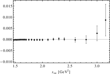
(a) First Weinberg sum rule, Eq. (10).

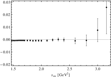
(b) Second Weinberg sum rule, Eq. (11).

Figure 1: Weinberg sum rules, Eqs. (10) and  (11). Data is used for $s<s_{\rm sw}$ and the DV Ansatz of Eq. (8) is used for $s>s_{\rm sw}$using results from a fit to $V$ and $A$ with moments of $w_{1}$, $w_{2}$, and $w_{3}$, within CIPT. The parameters are given in Tab. V of Ref. [22].

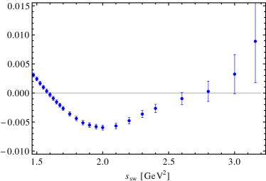
(a) First Weinberg sum rule, Eq. (10), without DVs.

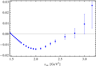
(b) Second Weinberg sum rule, Eq. (11), without DVs.

Figure 2: Weinberg sum rules, Eqs. (10) and (11) without the DV contribuiton. These results should be compared with Fig. 1 where the DV contribution is taken into account.

To illustrate the importance of the DVs we display in Fig. 2 the results for the Weinberg sum rules as a function of $s_{\rm sw}$ but without the DV contribution. The comparison between these two results gives us confidence that the DVs obtained from the data are sound since their extrapolation to infinity is in excellent agreement with the constraints from the Weinberg sum rules.

5 Conclusions

We have extracted $\alpha_{s}$ and non-perturbative parameters from the updated ALEPH data for hadronic $\tau$ decays. This extraction is sound and our results fulfill consistency tests. The $\alpha_{s}$ values can be averaged with those obtained from the OPAL data. The final results are given in Sec. 4.1. The ALEPH data constrain the DV parameters better than OPAL’s and our DV parameters fulfill the constraints imposed by Weinberg sum rules. Nevertheless, the non-perturbative physics limits the accuracy with which the strong coupling can be extracted.

References

- [1] E. Braaten, S. Narison, and A. Pich, Nucl. Phys. B 373 581 (1992).
- [2] R. Barate et al. [ALEPH Collaboration], Eur. Phys. J. C4, 409 (1998); S. Schael et al. [ALEPH Collaboration], Phys. Rept. 421, 191 (2005) [arXiv:hep-ex/0506072].
- [3] K. Ackerstaff et al. [OPAL Collaboration], Eur. Phys. J. C 7 571 (1999) [arXiv:hep-ex/9808019].
- [4] P. A. Baikov, K. G. Chetyrkin and J. H. Kühn, Phys. Rev. Lett. 101 012002 (2008) [arXiv:0801.1821 [hep-ph]].
- [5] K. Maltman, T. Yavin, Phys. Rev. D78, 094020 (2008) [arXiv:0807.0650 [hep-ph]].
- [6] M. Davier et al., Eur. Phys. J. C56, 305 (2008) [arXiv:0803.0979 [hep-ph]].
- [7] D. Boito, O. Cata, M. Golterman, M. Jamin, K. Maltman, J. Osborne and S. Peris, Phys. Rev. D84, 113006 (2011) [arXiv:1110.1127 [hep-ph]].
- [8] D. Boito, M. Golterman, M. Jamin, A. Mahdavi, K. Maltman, J. Osborne, and S. Peris, Phys. Rev. D 85, 093015 (2012) [arXiv:1203.3146 [hep-ph]].
- [9] D. R. Boito, O. Cata, M. Golterman, M. Jamin, K. Maltman, J. Osborne and S. Peris, Nucl. Phys. Proc. Suppl. 218, 104 (2011) [arXiv:1011.4426 [hep-ph]].
- [10] M. Davier, A. H cker, B. Malaescu, C. Z. Yuan and Z. Zhang, Eur. Phys. J. C 74, no. 3, 2803 (2014) [arXiv:1312.1501 [hep-ex]].
- [11] The spectral functions can be found in the following url: http://aleph.web.lal.in2p3.fr/tau/specfun13.html
- [12] A. A. Pivovarov, Z. Phys. C 53 461 (1992) [Sov. J. Nucl. Phys. 54 676 (1991)] [Yad. Fiz. 54 1114 (1991)] [arXiv:hep-ph/0302003]; F. Le Diberder, A. Pich, Phys. Lett. B289 165 (1992).
- [13] See, for instance, M. Jamin, JHEP 0509, 058 (2005) [hep-ph/0509001].
- [14] M. Beneke and M. Jamin, JHEP 0809, 044 (2008) [arXiv:0806.3156 [hep-ph]].
- [15] M. Beneke, D. Boito and M. Jamin, JHEP 1301, 125 (2013) [arXiv:1210.8038 [hep-ph]].
- [16] R. Shankar, Phys. Rev. D15, 755 (1977); R. G. Moorhose, M. R. Pennington and G. G. Ross, Nucl. Phys. B124, 285 (1977); K. G. Chetyrkin and N. V. Krasnikov, Nucl. Phys. B119, 174 (1977); K. G. Chetyrkin, N. V. Krasnikov and A. N. Tavkhelidze, Phys. Lett. 76B, 83 (1978); N. V. Krasnikov, A. A. Pivovarov and N. N. Tavkhelidze, Z. Phys. C19, 301 (1983); E. G. Floratos, S. Narison and E. de Rafael, Nucl. Phys. B155, 115 (1979); R. A. Bertlmann, G. Launer and E. de Rafael, Nucl. Phys. B250, 61 (1985).
- [17] B. Blok, M. A. Shifman and D. X. Zhang, Phys. Rev. D 57 2691 (1998) [Erratum-ibid. D 59 019901 (1999) ] [arXiv:hep-ph/9709333]; I. I. Y. Bigi, M. A. Shifman, N. Uraltsev, A. I. Vainshtein, Phys. Rev. D59, 054011 (1999) [hep-ph/9805241]; M. A. Shifman, [hep-ph/0009131].
- [18] O. Catà, M. Golterman, S. Peris, JHEP 0508, 076 (2005) [hep-ph/0506004].
- [19] O. Catà, M. Golterman, S. Peris, Phys. Rev. D77, 093006 (2008) [arXiv:0803.0246 [hep-ph]].
- [20] O. Catà, M. Golterman, S. Peris, Phys. Rev. D79, 053002 (2009) [arXiv:0812.2285 [hep-ph]].
- [21] M. Jamin, JHEP 1109, 141 (2011) [arXiv:1103.2718 [hep-ph]].
- [22] D. Boito, M. Golterman, K. Maltman, J. Osborne and S. Peris, Phys. Rev. D 91, no. 3, 034003 (2015) [arXiv:1410.3528 [hep-ph]].
- [23] S. Narison, V. I. Zakharov, Phys. Lett. B679, 355 (2009) [arXiv:0906.4312 [hep-ph]].
- [24] S. Narison, Phys. Lett. B673, 30 (2009) [arXiv:0901.3823 [hep-ph]].