Generalized Model of VSC-based Energy Storage Systems for Transient Stability Analysis

Abstract

This paper presents a generalized energy storage system model for voltage and angle stability analysis. The proposed solution allows modeling most common energy storage technologies through a given set of linear differential algebraic equations (DAEs). In particular, the paper considers, but is not limited to, compressed air, superconducting magnetic, electrochemical capacitor and battery energy storage devices. While able to cope with a variety of different technologies, the proposed generalized model proves to be accurate for angle and voltage stability analysis, as it includes a balanced, fundamental-frequency model of the voltage source converter (VSC) and the dynamics of the dc link. Regulators with inclusion of hard limits are also taken into account. The transient behavior of the generalized model is compared with detailed fundamental-frequency balanced models as well as commonly-used simplified models of energy storage devices. A comprehensive case study based on the WSCC 9-bus test system is presented and discussed.

I Introduction

The capability of Energy Storage Systems (ESSs) to improve the transient behavior of power systems and to increase the competitiveness of non-dispatchable power production technologies, e.g., renewable energies, has led, in recent years, to a huge investment in research, prototyping and installation of storage devices as well as the development of a huge variety of energy storage technologies [1, 2, 3]. Among most relevant technologies that currently appear most promising there are Battery Energy Storage (BES), Compressed Air Energy Storage (CAES), Superconducting Magnetic Energy storage (SMES), Electrochemical Capacitor Energy Storage (ECES), and Flywheel Energy Storage (FES).

Modeling ESSs is a complex and time-consuming task due to the number of different technologies that are currently available and that are expected to be developed in the future. While there are several studies aimed to define the economic viability and the effect on electricity markets of ESSs (see for example [2] and [4]), there is still no commonly-accepted simple yet accurate general model of ESSs for voltage and angle stability studies. This paper presents a generalized model of ESSs to simplify, without giving up accuracy, the simulation of different storage technologies. The objective is to provide a balanced, fundamental frequency model that can be defined through a reduced and fixed set of parameters and that can be readily implemented in power system simulators for voltage and angle stability analysis.

Studies that focus on ESS dynamic models aimed to transient stability analysis abound in the literature. The following are relevant works. A general taxonomy for ESS dynamic analysis is presented in [5]. A detailed transient stability model of ECES can be found in [6], while the model of SMES is given in [7]. Studies of the dynamic performance of a SMES system coupled to a wind power plant throughout a voltage source converter (VSC) are presented in [8] and [9], whereas information regarding the installation of a large-scale SMES at the Center of Advanced Power Systems at Florida State University can be found in [10]. In [11], the authors propose the model of a small-size CAES based on a polytropic process of air compression and expansion and in [12, 13] BES dynamic models are proposed and tested. Finally, transient stability models of FES can be found in [14] and [15].

Several simplified ESS models have been also proposed. Among these, we cite [16, 17, 18, 19, 20]. The main feature that the models proposed in the references above have in common is that the ESS dynamics are represented considering only active and reactive power controllers. However, the dynamics of the ESS itself are not preserved. These models are also generally loss-less as dc and VSC circuitry is neglected.

In this paper, we use the balanced, fundamental frequency model of the VSC that is proposed in [21, 22, 23, 24, 25], which includes dc circuit and phase-locked loop (PLL) dynamics as well as an average $dq$-axis model of the converter and an equivalent model for switching losses.

The model proposed is based on the observation that most ESSs connected to transmission and distribution grids share a common structure, i.e., are coupled to the ac network through a VSC device, present a dc-link and then include another converter (either a dc/dc or a ac/dc device) to connect the main energy storage device to the dc link. Moreover, all storage systems necessarily imply potential and flow quantities (see Table I), whose dynamics characterize the transient response of the ESS. In this paper, we show that, to properly capture the dynamic response of the ESS, it is important to preserve such dynamics along with those of the VSC converter and its controllers. Controller hard limits, whose relevance has been discussed in [20] and [26], are also considered.

TABLE I: Examples of energy storage technologies.

Types of	Potential Var.	Flow Var.	Device
Storable Energy
Magnetic	Magneto Motive	Flux	SMES
	Force
Fluid	Pressure	Mass Flow	CAES
Electrostatic	Electric Potential	Electric Current	ECES
Electrochemical	Electrochemical	Molar Flow	BES
	Potential	Rate
Rotational	Angular Velocity	Torque	FES

In summary, the paper provides the following contributions:

1. A simple yet accurate generalized storage device model that consists of a given set of parameters and linear differential algebraic equations (DAEs). This model is characterized by a given set of DAEs whose structure and dynamic order is independent from the technology used for the ESS.

2. A balanced, fundamental frequency model of the typical devices that compose an ESS, namely, the VSC, the dc link and their regulators. This model is obtained based on a careful selection of well-assessed models for transient stability analysis.

3. A comprehensive validation of the dynamic response of the proposed ESS model versus detailed transient stability models representing specific technologies as well as simplified models that include only active and reactive power controllers.

The paper is organized as follows. Section II outlines the structure of a generic VSC-based ESS. The schemes of the regulators that are common to all ESSs, as well as the active and reactive controllers used for simplified ESS models are also presented in this section. Section III describes the hypotheses, the structure and the formulation of the proposed generalized model of ESS, as well as how this model is able to describe the behavior of a variety of ESS technologies. Section IV compares the dynamic response of the proposed model with detailed and simplified models of ESSs for transient stability analysis. All simulations are based on the WSCC 9-bus test system. Finally, section V draws conclusions and outlines future work directions.

II ESS Controls and Simplified ESS Model

This section presents the elements and controllers that regulate the dynamic response of the ESS. In this section, we consider exclusively the elements of the ESS model that are independent from the storage technology. We also present the simplified ESS model that is used for comparison in the case study presented in Section IV.

II-A Detailed ESS scheme for Transient Stability Analysis

Figure 1 shows the overall structure of an ESS connected to a grid through a VSC. The objective of the ESS is to control a measured quantity w, e.g., the frequency of the Center of Inertia (COI) or the power flowing through a transmission line. The elements shown in Fig. 1 are common to all VSC-based ESSs. The models of these elements, except for the storage device, are presented in the remainder of this section.

\psfrag{ESS}{\LARGE{Storage}}\psfrag{Grid}{\LARGE{Grid}}\psfrag{Storage Control}{\Large{Storage Control}}\psfrag{VSC Control}{\Large{VSC Control}}\psfrag{vac}{\LARGE{$v_{\rm ac}$}}\psfrag{vacref}{\LARGE{$v_{\rm ac}^{\rm ref}$}}\psfrag{vdc}{\LARGE{$v_{\rm dc}$}}\psfrag{idc}{\LARGE{$i_{\rm dc}$}}\psfrag{iac}{\LARGE{$i_{\rm ac}$}}\psfrag{vdcref}{\LARGE{$v_{\rm dc}^{\rm ref}$}}\psfrag{+}{\Large{$+$}}\psfrag{-}{\Large{$-$}}\psfrag{w}{\LARGE{$\textit{w}$}}\psfrag{wref}{\LARGE{$\textit{w}^{\rm ref}$}}\psfrag{u}{\LARGE{$u$}}\psfrag{uref}{\LARGE{$u^{\rm ref}$}}\psfrag{a}{\LARGE{$m_{\rm d}$}}\psfrag{b}{\LARGE{$m_{\rm q}$}}\includegraphics{essvsc2}

Figure 1: Scheme of the ESS connected to a grid.

Figure 2 illustrates the VSC scheme [21, 22, 23]. The usual configuration includes a transformer, a bi-directional converter and a condenser. The transformer provides galvanic insulation, whereas the condenser maintains the voltage level at the dc side of the converter. The dc voltage is converted to ac voltage waveform via the use of power electronic converters that are controlled using appropriate control logic.

\psfrag{+}{\footnotesize{$+$}}\psfrag{-}{\footnotesize{$-$}}\psfrag{v}{\small{$v_{\rm dc}$}}\psfrag{i}{\small{$i_{\rm dc}$}}\psfrag{C}{\small{$C_{\rm dc}$}}\psfrag{L}{\small{$L_{\rm ac}$}}\psfrag{R}{\small{$R_{\rm ac}$}}\psfrag{G}{\small{$G_{\rm sw}(i_{\rm dc})$}}\psfrag{p}{\small{$p_{\rm ac}+jq_{\rm ac}$}}\psfrag{vac}{\small{$v_{\rm ac}\angle\theta_{\rm ac}$}}\psfrag{vt}{\small{$v_{\rm t}\angle\theta_{\rm t}$}}\psfrag{vdc}{\small{$\sqrt{\frac{3}{8}}a_{\rm m}v_{\rm dc}$}}\includegraphics[width=227.62204pt]{VSC}

Figure 2: VSC scheme.

\psfrag{+}{\footnotesize{$+$}}\psfrag{-}{\footnotesize{$-$}}\psfrag{idref}{\footnotesize{$i_{\rm ac,d}^{\rm ref}$}}\psfrag{iqref}{\footnotesize{$i_{\rm ac,q}^{\rm ref}$}}\psfrag{id}{\footnotesize{$i_{\rm ac,d}$}}\psfrag{iq}{\footnotesize{$i_{\rm ac,q}$}}\psfrag{Ki}{\footnotesize{$K_{\rm I}(s)$}}\psfrag{wliq}{\scriptsize{$\omega_{\rm ac}L_{\rm ac}i_{\rm ac,q}$}}\psfrag{wlid}{\scriptsize{$\omega_{\rm ac}L_{\rm ac}i_{\rm ac,d}$}}\psfrag{vacd}{\footnotesize{$v_{\rm ac,d}$}}\psfrag{vacq}{\footnotesize{$v_{\rm ac,q}$}}\psfrag{2vdc}{\large{$\frac{2}{v_{\rm dc}}$}}\psfrag{vdc2}{\large{$\frac{v_{\rm dc}}{2}$}}\psfrag{md}{\footnotesize{$m_{\rm d}$}}\psfrag{mq}{\footnotesize{$m_{\rm q}$}}\psfrag{vtd}{\scriptsize{$v_{\rm t,d}$}}\psfrag{vtq}{\scriptsize{$v_{\rm t,q}$}}\psfrag{w}{\footnotesize{$\omega_{\rm ac}$}}\psfrag{1}{\footnotesize{$1$}}\psfrag{RsL}{\scriptsize{$R_{\rm ac}$+$sL_{\rm ac}$}}\psfrag{L}{\footnotesize{$L_{\rm ac}$}}\psfrag{inner control}{\scriptsize{Inner Current Control Loop}}\psfrag{converter}{\scriptsize{Converter}}\includegraphics[width=227.62204pt]{vsccoupling}

Figure 3: Block diagram of the inner current control and the converter in the $dq$-frame.

Figure 3 shows the block diagram representation of both the converter and the inner current control loop of the VSC. After transforming the three-phase equations to a rotating $dq$-frame, the dynamics of the ac side of the VSC depicted in Fig. 2 become:

$$\begin{array}[]{lll}R_{\rm ac}i_{\rm ac,d}+L_{\rm ac}\dfrac{di_{\rm ac,d}}{dt}=\hskip 6.82881pt\omega_{\rm ac}L_{\rm ac}i_{\rm ac,q}+v_{\rm ac,d}\vspace*{0.15cm}-v_{\rm t,d}\\ R_{\rm ac}i_{\rm ac,q}+L_{\rm ac}\dfrac{di_{\rm ac,q}}{dt}=-\omega_{\rm ac}L_{\rm ac}i_{\rm ac,d}+v_{\rm ac,q}-v_{\rm t,q}\end{array}$$ (1)

where $R_{\rm ac}+jL_{\rm ac}$ is the aggregated impedance of the converter reactance and transformer; $v_{\rm t,d}=m_{\rm d}v_{\rm dc}/2$; $v_{\rm t,q}=m_{\rm q}v_{\rm dc}/2$; and $\omega_{\rm ac}$ is the frequency of the grid voltage, $\bar{v}_{\rm ac}$.

It is possible to express dc signals in a $dq$-reference frame, with the aim of designing suitable controllers, provided that the $dq$-reference frame rotates with the same speed as the grid voltage phasor, which may be achieved, for example, through the use of a phase-locked loop (PLL) [24]. The PLL is a control system that forces the angle of the rotating $dq$-frame, $\theta_{dq}$, to track the angle $\theta_{\rm ac}$. The PLL is typically composed of a phase detector (PD), a loop filter (LF), and a voltage controlled oscillator (VCO), and its scheme is depicted in Fig. 4.

\psfrag{-}{\small{$-$}}\psfrag{ti}{\small{$\theta_{\rm ac}$}}\psfrag{to}{\small{$\theta_{dq}$}}\psfrag{K1}{\small{$K_{\rm PD}$}}\psfrag{sa}{\small{$1+sT_{\rm 1,LF}$}}\psfrag{sb}{\small{$sT_{\rm 2,LF}$}}\psfrag{K2}{\small{$K_{\rm VCO}$}}\psfrag{s}{\small{$s$}}\includegraphics[width=227.62204pt]{pll}

Figure 4: PLL scheme.

The grid voltage $\bar{v}_{\rm ac}$ can, thus, be expressed in the $dq$-frame as follows:

$$v_{\rm ac,d}+jv_{\rm ac,q}=v_{\rm ac}(\cos(\theta_{\rm ac}-\theta_{dq})+j\sin(\theta_{\rm ac}-\theta_{dq}))$$ (2)

The controller $K_{\rm I}(s)$ of Fig. 3 is designed as a PI control, as follows [21]:

$$K_{\rm I}(s)=\dfrac{R_{\rm ac}+sL_{\rm ac}}{sT_{\rm I}}$$ (3)

where $T_{\rm I}$ is the time-constant of the closed-loop step response.

The power balance between the dc and the ac sides of the converter is imposed by:

$$p_{\rm ac}+v_{\rm dc}i_{\rm dc}-p_{\rm loss}-\dfrac{1}{2}C_{\rm dc}\dfrac{d(v_{\rm dc}^{2})}{dt}=0$$ (4)

where $p_{\rm ac}=\dfrac{3}{2}(v_{\rm ac,d}i_{\rm ac,d}+v_{\rm ac,q}i_{\rm ac,q})$; $\dfrac{1}{2}C_{\rm dc}\dfrac{d(v_{\rm dc}^{2})}{dt}$ are the energy variations in the capacitor; and $p_{\rm loss}=\dfrac{3}{2}R_{\rm ac}i_{\rm ac}^{2}+G_{\rm sw}(i_{\rm dc})v_{\rm dc}^{2}$ are the circuit and switching losses of the converter, respectively, with $i_{\rm ac}^{2}=i_{\rm ac,d}^{2}+i_{\rm ac,q}^{2}$; and $G_{\rm sw}(i_{\rm dc})$ is obtained from a given constant conductance, $G_{0}$, and the quadratic ratio of the actual current to the nominal one, as follows [25]:

$$G_{\rm sw}(i_{\rm dc})=G_{0}\left(\frac{i_{\rm dc}}{i_{\rm dc}^{\rm nom}}\right)^{2}$$ (5)

Finally, the outer controllers used to regulate the dc and ac voltages of the VSC are depicted in Fig. 5.

\psfrag{vac}{$v_{\rm ac}$}\psfrag{vdc}{$v_{\rm dc}$}\psfrag{Kmdc}{$K_{\rm mdc}$}\psfrag{Tmdc}{$1+sT_{\rm mdc}$}\psfrag{vmdc}{$v_{\rm mdc}$}\psfrag{vdcref}{$v_{\rm dc}^{\rm ref}$}\psfrag{+}{\tiny{$+$}}\psfrag{-}{\tiny{$-$}}\psfrag{PI}{PI control}\psfrag{Kp}{$K_{\rm d}$}\psfrag{Ki}{$K_{\rm i,d}$}\psfrag{xd}{$x_{\rm d}$}\psfrag{s}{$s$}\psfrag{idmax}{$i_{\rm d}^{\rm ref,max}$}\psfrag{idmin}{$i_{\rm d}^{\rm ref,min}$}\psfrag{idref}{$i_{\rm d}^{\rm ref}$}\psfrag{Kmac}{$K_{\rm mac}$}\psfrag{Tmac}{$1+sT_{\rm mac}$}\psfrag{vmac}{$v_{\rm mac}$}\psfrag{vacref}{$v_{\rm ac}^{\rm ref}$}\psfrag{+}{\tiny{$+$}}\psfrag{-}{\tiny{$-$}}\psfrag{leadlag}{lead/lag control}\psfrag{K}{$K_{\rm q}$}\psfrag{KdT2}{$K_{\rm d,q}+sT_{2}$}\psfrag{xq}{$x_{\rm q}$}\psfrag{T1}{$1+sT_{1}$}\psfrag{iqmax}{$i_{\rm q}^{\rm ref,max}$}\psfrag{iqmin}{$i_{\rm q}^{\rm ref,min}$}\psfrag{iqref}{$i_{\rm q}^{\rm ref}$}\includegraphics[width=256.0748pt]{vscoutercontrol}

Figure 5: Outer dc and ac voltage controllers.

The charge/discharge process of the storage device is regulated by the storage control (see Fig. 6). The input signal of the control is the error between the actual value of a measured quantity of the system, say w, and a reference value ($\textit{w}^{\rm ref}$). If $\textit{w}=\textit{w}^{\rm ref}$, the storage device is inactive and its energy is kept constant. For $\textit{w}\neq\textit{w}^{\rm ref}$, the storage device injects active power into the ac bus through the VSC (discharge process) or absorbs power from the ac bus (charge process). The scheme shown in Fig. 6 also includes a block referred to as Storage Input Limiter[26]. The purpose of this limiter is to smooth the transients that derive from energy saturations of the storage device. This block takes the actual value of the energy stored in the device, $E$, and defines the value of the controlled input variable of the storage device, $u$, as follows:

$$u=\left\{\begin{array}[]{l}\displaystyle\frac{E-E_{\rm min}}{E_{\rm min}^{\rm thr}-E_{\rm min}}\Delta u+u_{\rm ref}\vspace*{0.2cm}\\ \vspace*{0.2cm}\quad\quad\text{if}\quad E_{\rm min}\leq E\leq E_{\rm min}^{\rm thr}\quad\text{and}\quad\Delta u>0\\ \vspace*{0.2cm}\displaystyle\frac{E_{\rm max}-E}{E_{\rm max}-E_{\rm max}^{\rm thr}}\Delta u+u_{\rm ref}\\ \vspace*{0.2cm}\quad\quad\text{if}\quad E_{\rm max}^{\rm thr}\leq E\leq E_{\rm max}\quad\text{and}\quad\Delta u<0\\ \displaystyle\hat{u}\quad\text{otherwise}\\ \end{array}\right.$$ (6)

where $u_{\rm ref}$ is the value of $u$ such that the storage device is disabled; $\Delta u=\hat{u}-u_{\rm ref}$; $E_{\rm min}$ and $E_{\rm max}$ are the minimum and maximum storable energy in the ESS, respectively; and $E_{\rm min}^{\rm thr}$ and $E_{\rm max}^{\rm thr}$ are the given minimum and maximum energy thresholds, respectively.

\psfrag{w}{\huge$\textit{w}$}\psfrag{wref}{\huge$\textit{w}^{\rm ref}$}\psfrag{E}{\LARGE$E$}\psfrag{du}{\huge$|\Delta u|$}\psfrag{DB}{\huge Dead-band}\psfrag{Ulimit}{\huge Storage Input Limiter}\psfrag{1}{\huge$1$}\psfrag{1 }{\huge$1$}\psfrag{0}{\huge$0$}\psfrag{Tf}{\huge$1$+$sT_{\rm f}$}\psfrag{xdp}{\huge$x_{\rm f}$}\psfrag{+}{}\psfrag{-}{{\large$-$}}\psfrag{PI}{\huge PI control}\psfrag{Kp}{\huge$K_{{\rm p}u}$}\psfrag{Ki}{\huge$K_{{\rm i}u}$}\psfrag{xi}{\huge$x_{u}$}\psfrag{Hd}{\huge$s$}\psfrag{umax}{\huge$u^{\rm max}$}\psfrag{umin}{\huge$u^{\rm min}$}\psfrag{u}{\huge$u$}\psfrag{uhat}{\huge$\hat{u}$}\psfrag{uref}{\huge$u_{\rm ref}$}\includegraphics{storagecontrol}

Figure 6: Storage control scheme.

A dead-band block is also included in Fig. 6. This block is designed to reduce the sensitivity of the Storage Control to small changes of the measured signal w with respect to the reference $\textit{w}^{\rm ref}$. The purpose of the dead-band is to reduce the number of charge/discharge operations of the ESS [9].

II-B Simplified ESS scheme

As discussed in Section I, several simplified models of ESSs have been proposed [16, 17, 18, 19, 20]. For the sake of comparison, in this paper, we consider the control scheme proposed in [16] (see Fig. 7). The input signal w is regulated through the active power while the voltage at the point of connection with the grid is regulated through the ESS reactive power. The physical behavior of the storage system is synthesized by the two lag blocks with time constants $T_{P,\rm ESS}$ and $T_{Q,\rm ESS}$.

\psfrag{w}{$\textit{w}$}\psfrag{wref}{$\textit{w}^{\rm ref}$}\psfrag{1}{$1$}\psfrag{Tfp}{$1+sT_{\rm f\it{P}}$}\psfrag{xfp}{$x_{\rm f\it{P}}$}\psfrag{+}{\tiny{$+$}}\psfrag{-}{\tiny{$-$}}\psfrag{PI}{PI control}\psfrag{Kp}{$K_{\rm p\it{P}}$}\psfrag{Ki}{$K_{\rm i\it{P}}$}\psfrag{xp}{$x_{P}$}\psfrag{Hd}{$s$}\psfrag{Tp}{$1+sT_{P,\rm ESS}$}\psfrag{P}{$P_{\rm ESS}$}\psfrag{Pmax}{$P_{\rm ESS}^{\max}$}\psfrag{Pmin}{$P_{\rm ESS}^{\min}$}\psfrag{v}{$v_{\rm ac}$}\psfrag{vref}{$v_{\rm ac}^{\rm ref}$}\psfrag{Tfq}{$1+sT_{\rm f\it{Q}}$}\psfrag{xfq}{$x_{\rm{f}\it{Q}}$}\psfrag{leadlag}{lead/lag control}\psfrag{Kq}{$K_{Q}$}\psfrag{T2}{$1+sT_{Q2}$}\psfrag{T1}{$1+sT_{Q1}$}\psfrag{Tq}{$1+sT_{Q\rm,ESS}$}\psfrag{Q}{$Q_{\rm ESS}$}\psfrag{Qmax}{$Q_{\rm ESS}^{\max}$}\psfrag{Qmin}{$Q_{\rm ESS}^{\min}$}\includegraphics[width=256.0748pt]{SimplifiedModel.eps}

Figure 7: Scheme of a simplified ESS model.

III Proposed Generalized Model of Energy Storage Devices

The generalized model proposed in this paper is based on the linearization and dynamic reduction of the set of equations that describes the storage device. Let assume that the dynamic behavior of the ESS can be described by a set of nonlinear DAE as follows:

$$\boldsymbol{\Gamma}\dot{\boldsymbol{\xi}}(t) =\boldsymbol{\psi}(\boldsymbol{\xi}(t),\boldsymbol{\nu}(t))$$

$$\boldsymbol{\varphi}(t) =\boldsymbol{\eta}(\boldsymbol{\xi}(t),\boldsymbol{\nu}(t))$$ (7)

where $\boldsymbol{\xi}(t)$ is the state vector ($\boldsymbol{\xi}\in\mathbb{R}^{n}$); $\boldsymbol{\nu}(t)$ is the input vector ($\boldsymbol{\nu}\in\mathbb{R}^{m}$); $\boldsymbol{\varphi}(t)$ is the output vector ($\boldsymbol{\varphi}\in\mathbb{R}^{p}$); $\boldsymbol{\psi}:\mathbb{R}^{n+m}\rightarrow\mathbb{R}^{n}$ are the differential equations; $\boldsymbol{\eta}:\mathbb{R}^{n+m}\rightarrow\mathbb{R}^{p}$ are the output equations; and $\boldsymbol{\Gamma}$ is a diagonal matrix of dimensions $n\times n$ such that [27]:

• $\boldsymbol{\Gamma}_{ii}=1$ if the $i$-th equation of $\boldsymbol{\psi}$ is differential;

• $\boldsymbol{\Gamma}_{ii}=0$ if the $i$-th equation of $\boldsymbol{\psi}$ is algebraic.

The first step towards the definition of the generalized model of the ESS is to linearize the system around the equilibrium point ($\boldsymbol{\xi}_{0},\boldsymbol{\varphi}_{0},\boldsymbol{\nu}_{0}$). Thus, the expression for a linear time-invariant dynamical system is obtained:

$$\boldsymbol{\Gamma}\dot{\boldsymbol{\xi}}(t) =\mathbf{A}\boldsymbol{\xi}(t)+\mathbf{B}\boldsymbol{\nu}(t)+\mathbf{K}_{\xi}$$

$$\boldsymbol{\varphi}(t) =\mathbf{C}\boldsymbol{\xi}(t)+\mathbf{D}\boldsymbol{\nu}(t)+\mathbf{K}_{\varphi}$$ (8)

where $\mathbf{A}$ is the state matrix $\left({\rm dim}[\mathbf{A}]=n\times n\right)$; $\mathbf{B}$ is the input matrix $\left({\rm dim}[\mathbf{B}]=n\times m\right)$; $\mathbf{C}$ is the output matrix $\left({\rm dim}[\mathbf{C}]=p\times n\right)$; $\mathbf{D}$ is the feedthrough matrix $\left({\rm dim}[\mathbf{D}]=p\times m\right)$; and $\mathbf{K}_{\xi}\in\mathbb{R}^{n}$ and $\mathbf{K}_{\varphi}\in\mathbb{R}^{p}$ account for the values of the variables at the equilibrium point. Equation (8) is written for $\boldsymbol{\xi}$, $\boldsymbol{\nu}$ and $\boldsymbol{\varphi}$, not the incremental values $\Delta\boldsymbol{\xi}$, $\Delta\boldsymbol{\nu}$, and $\Delta\boldsymbol{\varphi}$.

Then, the state vector $\boldsymbol{\xi}$ is split into two types of variables: the potential and flow variables related to the energy stored in the ESS, $\boldsymbol{x}$ (see Table I); and all other state variables, $\boldsymbol{z}$. Hence, $\boldsymbol{\xi}=[\boldsymbol{x}^{T},\;\boldsymbol{z}^{T}]^{T}$. Since all ESSs are coupled to the ac network through a VSC device, the dc voltage and current of the VSC, $v_{\rm dc}$ and $i_{\rm dc}$, are considered as an input and an output in (8), respectively. The input vector $\boldsymbol{\nu}$ is composed of the output signals of the storage control, $u$, and the dc voltage of the VSC, $v_{\rm dc}$. Hence, $\boldsymbol{\nu}=[u,\;v_{\rm dc}]^{\rm T}$. Finally, the output vector $\boldsymbol{\varphi}$ is the dc current of the VSC, $i_{\rm dc}$. Hence, $\boldsymbol{\varphi}=[i_{\rm dc}]$. Applying the notation above, equation (8) is written as follows:

$$\mathbf{\Gamma}_{x}\dot{\boldsymbol{x}} =\mathbf{A}_{xx}\boldsymbol{x}+\mathbf{A}_{xz}\boldsymbol{z}+\mathbf{B}_{xu}u+\mathbf{B}_{xv}v_{\rm dc}+\mathbf{K}_{x}$$

$$\mathbf{\Gamma}_{z}\dot{\boldsymbol{z}} =\mathbf{A}_{zx}\boldsymbol{x}+\mathbf{A}_{zz}\boldsymbol{z}+\mathbf{B}_{zu}u+\mathbf{B}_{zv}v_{\rm dc}+\mathbf{K}_{z}$$ (9)

$$i_{\rm dc} =\mathbf{C}_{x}\boldsymbol{x}+\mathbf{C}_{z}\boldsymbol{z}+\mathbf{D}_{u}u+\mathbf{D}_{v}v_{\rm dc}+\mathbf{K}_{i}$$

where:

• ${\scriptscriptstyle{\begin{bmatrix}\mathbf{A}_{xx}&\mathbf{A}_{xz}\\ \mathbf{A}_{zx}&\mathbf{A}_{zz}\end{bmatrix}}}=\mathbf{A}$ ;  ${\scriptscriptstyle{\begin{bmatrix}\mathbf{B}_{xu}&\mathbf{B}_{xv}\\ \mathbf{B}_{zu}&\mathbf{B}_{zv}\end{bmatrix}}}=\mathbf{B}$ ;

• $[\mathbf{C}_{x}\;\mathbf{C}_{z}]=\mathbf{C}$ ;   $[\mathbf{D}_{u}\;\mathbf{D}_{v}]=\mathbf{D}$ ;

• $[\mathbf{\Gamma}_{x}\;\mathbf{\Gamma}_{z}]^{T}=\mathbf{\Gamma}$ ;   $[\mathbf{K}_{x}\;\mathbf{K}_{z}]^{T}=\mathbf{K}_{\xi}$ ;   $\mathbf{K}_{i}=\mathbf{K}_{\varphi}$

The dynamic order of (9) is reduced by assuming that the transient response of $\boldsymbol{z}$ are much faster than that of $\boldsymbol{x}$ or immaterial with respect to the overall dynamic behavior of the ESS. This assumption is based on the knowledge of detailed transient stability models and is duly verified through the simulations presented in Section IV. By neglecting the dynamics of $\boldsymbol{z}$ (i.e., $\mathbf{\Gamma}_{z}=\mathbf{0}$), from the second equation of (9), we obtain:

$$\boldsymbol{z}=-\mathbf{A}_{zz}^{-1}\left(\mathbf{A}_{zx}\boldsymbol{x}+\mathbf{B}_{zu}u+\mathbf{B}_{zv}v_{\rm dc}+\mathbf{K}_{z}\right)$$ (10)

Then, substituting (10) into the first and third equations of (9), one has:

$$\mathbf{\Gamma}_{x}\dot{\boldsymbol{x}} =\left(\mathbf{A}_{xx}-\mathbf{A}_{xz}\mathbf{A}_{zz}^{-1}\mathbf{A}_{zx}\right)\boldsymbol{x}+\left(\mathbf{B}_{xu}-\mathbf{A}_{xz}\mathbf{A}_{zz}^{-1}\mathbf{B}_{zu}\right)u$$

$$+\left(\mathbf{B}_{xv}-\mathbf{A}_{xz}\mathbf{A}_{zz}^{-1}\mathbf{B}_{zv}\right)v_{\rm dc}+\left(\mathbf{K}_{x}-\mathbf{A}_{xz}\mathbf{A}_{zz}^{-1}\mathbf{K}_{z}\right)$$

$$i_{\rm dc} =\left(\mathbf{C}_{x}-\mathbf{C}_{z}\mathbf{A}_{zz}^{-1}\mathbf{A}_{zx}\right)\boldsymbol{x}+\left(\mathbf{D}_{u}-\mathbf{C}_{z}\mathbf{A}_{zz}^{-1}\mathbf{B}_{zu}\right)u$$

$$+\left(\mathbf{D}_{v}-\mathbf{C}_{z}\mathbf{A}_{zz}^{-1}\mathbf{B}_{zv}\right)v_{\rm dc}+\left(\mathbf{K}_{i}-\mathbf{C}_{z}\mathbf{A}_{zz}^{-1}\mathbf{K}_{z}\right)$$ (11)

Rewriting in compact form the matrices in (11), the proposed generalized model of energy storage devices can be written as follows:

$$\tilde{\mathbf{\Gamma}}\dot{\boldsymbol{x}} = \tilde{\mathbf{A}}\boldsymbol{x}+\tilde{\mathbf{B}}_{u}u+\tilde{\mathbf{B}}_{v}v_{\rm dc}+\tilde{\mathbf{K}}_{x}$$

$$i_{\rm dc} = \tilde{\mathbf{C}}\boldsymbol{x}+\tilde{\mathbf{D}}_{u}u+\tilde{\mathbf{D}}_{v}v_{\rm dc}+\tilde{\mathbf{K}}_{i}$$ (12)

It is important to take into account the state of charge of the storage device (in particular, to impose energy limits to the controller shown in Fig. 6). With this aim, the actual stored energy is given by:

$$E=\sum_{\rm i=1}^{n}\rho_{\rm i}\left(x_{\rm i}^{\beta_{\rm i}}-\chi_{\rm i}^{\beta_{\rm i}}\right)$$ (13)

where $\rho_{\rm i}$, $\beta_{\rm i}$ and $\chi_{\rm i}$ are the proportional coefficient, exponential coefficient and reference potential value of each variable $x_{\rm i}$, respectively.

In summary, the proposed generalized ESS model is composed of the block diagram of the VSC represented in Fig. 3; the controllers depicted in Figs. 5 and 6; and (12), (13).

For the sake of clarity and example, in the following subsections we deduce the generalized model for a variety of ESSs technologies.

III-A Electrochemical Capacitor Energy Storage Model

Figure 8 shows the scheme of an ECES connected to the VSC through a bidirectional dc/dc converter (buck-boost) [6]. In the buck operation mode, the energy is delivered from the storage device to the grid, while in the boost mode, the energy is stored in the ECES.

\psfrag{Vsc}{{\large$v_{\rm sc}$}}\psfrag{Gsc}{{\large$G_{\rm sc}$}}\psfrag{Lsc}{{\large$L_{\rm sc}$}}\psfrag{Rsc}{{\large$R_{\rm sc}$}}\psfrag{Isc}{{\large$i_{\rm sc}$}}\psfrag{Csc}{{\large$C_{\rm sc}$}}\psfrag{DC}{{\large$\rm DC$}}\psfrag{Vdc}{{\large$v_{\rm dc}$}}\psfrag{Idc}{{\large$i_{\rm dc}$}}\psfrag{+}{$+$}\psfrag{-}{$-$}\psfrag{S}{{\large$S$}}\includegraphics[width=213.39566pt]{sces}

Figure 8: Scheme of an ECES.

The model that describes both the buck and the boost operation modes is as follows:

$$\dot{v}_{\rm sc} = -\frac{1}{C_{\rm sc}}\left(i_{\rm sc}+G_{\rm sc}v_{\rm sc}\right)$$

$$\dot{i}_{\rm sc} = \ \frac{1}{L_{\rm sc}}\left(v_{\rm sc}-i_{\rm sc}R_{\rm sc}-v_{\rm dc}S\right)$$ (14)

$$i_{\rm dc} = \ Si_{\rm sc}$$

where $S$ is the logic state of the switches of the converter. Assuming average variable values, $S$ is continuous and represents the duty cycle of the converter.

The energy stored in the ECES is as follows:

$$E=\frac{1}{2}C_{\rm sc}v_{\rm sc}^{2}+\frac{1}{2}L_{\rm sc}i_{\rm sc}^{2}$$ (15)

In (15), the main term is that related to the capacitance $C_{\rm sc}$, as expected. However, for completeness, we include also the energy stored in the inductance $L_{\rm sc}$.

Applying the notation of the proposed general model (12-13) to (14-15), ECES variables and parameters are:

$$\boldsymbol{x}=[v_{\rm sc}\;\;i_{\rm sc}]^{T};\;\boldsymbol{z}=\emptyset;\;\;u=S;\;\;\tilde{\mathbf{\Gamma}}={\scriptscriptstyle{\begin{bmatrix}1&0\\ 0&1\end{bmatrix}}};$$

$$\tilde{\mathbf{A}}={\scriptscriptstyle{\begin{bmatrix}-\frac{G_{\rm sc}}{C_{\rm sc}}&-\frac{1}{C_{\rm sc}}\\ \frac{1}{L_{\rm sc}}&-\frac{R_{\rm sc}}{L_{\rm sc}}\end{bmatrix}}};\ \tilde{\mathbf{B}}_{u}=\left[0\;\;\frac{v_{\rm dc,0}}{L_{\rm sc}}\right]^{T};\;\tilde{\mathbf{B}}_{v}=\left[0\;\;\frac{S_{\rm 0}}{L_{\rm sc}}\right]^{T};$$

$$\tilde{\mathbf{K}}_{x}={\scriptscriptstyle{\begin{bmatrix}\frac{1}{C_{\rm sc}}\left(G_{\rm sc}v_{\rm sc,0}+i_{\rm sc,0}\right)\\ \frac{1}{L_{\rm sc}}\left(-v_{\rm sc,0}+R_{\rm sc}i_{\rm sc,0}+2v_{\rm dc,0}S_{\rm 0}\right)\end{bmatrix}}};\;\tilde{\mathbf{C}}=[0\;\;S_{\rm 0}];$$

$$\tilde{\mathbf{D}}_{u}=[i_{\rm sc,0}];\ \tilde{\mathbf{D}}_{v}=[0];\ \tilde{\mathbf{K}}_{i}=[i_{\rm dc,0}-2S_{\rm 0}i_{\rm sc,0}];$$

$$\boldsymbol{\rho}=\left[\frac{1}{2}C_{\rm sc}\;\;\frac{1}{2}L_{\rm sc}\right];\ \boldsymbol{\beta}=[2\;\;2];\ \boldsymbol{\chi}=[0\;\;0]$$

where $S_{\rm 0}$, $v_{\rm sc,0}$, $v_{\rm dc,0}$, $i_{\rm sc,0}$ and $i_{\rm dc,0}$ are the values of $S$, $v_{\rm sc}$, $v_{\rm dc}$, $i_{\rm sc}$ and $i_{\rm dc}$ at the equilibrium point, respectively.

III-B Superconducting Magnetic Energy Storage Model

Figure 9 depicts the scheme of a SMES [7]. The SMES is connected in parallel to the VSC throughout a dc/dc converter (boost converter). The SMES stores magnetic energy and injects it into the network according to the duty cycle applied to the converter.

\psfrag{Ic}[c][c]{\Huge$i_{\rm c}$}\psfrag{Vc}[c][c]{\Huge$v_{\rm c}$}\psfrag{Idc}[c][c]{\Huge$i_{\rm dc}$}\psfrag{Vdc}[c][c]{\Huge$v_{\rm dc}$}\psfrag{DC}[c][c]{\Huge$\rm DC$}\psfrag{S}[c][c]{\Huge$S$}\psfrag{+}[c][c]{\LARGE$+$}\psfrag{-}[c][c]{\LARGE$-$}\includegraphics{smes}

Figure 9: Scheme of the SMES and the boost converter.

The dynamics of the coil and the dc/dc converter are represented by the circuit equations:

$$\dot{i}_{\rm c} = -\frac{v_{\rm c}}{L_{\rm c}}$$

$$\ 0 = \ (1-2S)v_{\rm dc}-v_{\rm c}$$ (16)

$$i_{\rm dc} = \ (1-2S)i_{\rm c}$$

where all voltages and currents are average values; $L_{\rm c}$ is the inductance of the superconducting coil; and $S$ is the duty cycle of the dc/dc converter.

The energy stored in the SMES is given by:

$$E=\frac{1}{2}L_{\rm c}i_{\rm c}^{2}$$ (17)

Therefore, using the notation of the proposed model:

$$\boldsymbol{x}=[i_{\rm c}\;\;v_{\rm c}]^{T};\;\boldsymbol{z}=\emptyset;\;\;u=S;\;\;\tilde{\mathbf{\Gamma}}={\scriptscriptstyle{\begin{bmatrix}1&0\\ 0&0\end{bmatrix}}}$$

$$\boldsymbol{\rho}=\left[\frac{1}{2}L_{\rm c}\;\;0\right];\;\;\boldsymbol{\beta}=\left[2\;\;1\right];\;\;\boldsymbol{\chi}=\left[0\;\;0\right]$$ (18)

III-C Compressed Air Energy Storage Model

The basic configuration of a CAES is represented in Fig. 10 [11]. The air is injected into the tank by means of a compressor operated by an asynchronous motor, and extracted from it through a turbine driven by an asynchronous generator. Both the compressor and the turbine are connected in parallel to the dc link of the VSC through ac/dc converters.

\psfrag{TANK}{\huge$\rm TANK$}\psfrag{COMP}{\huge$\rm COMP$}\psfrag{TURB}{\huge$\rm TURB$}\psfrag{AC}{\LARGE$\rm AC$}\psfrag{DC}{\LARGE$\rm DC$}\psfrag{+}{\Large$+$}\psfrag{-}{\Large$-$}\psfrag{vt}{\Huge$v_{\rm dc}$}\psfrag{it}{\Huge$i_{\rm dc,t}$}\psfrag{at}{\Huge$\hat{m}_{\rm d,t}$}\psfrag{bt}{\Huge$\hat{m}_{\rm q,t}$}\psfrag{vc}{\Huge$v_{\rm dc}$}\psfrag{ic}{\Huge$i_{\rm dc,c}$}\psfrag{ac}{\Huge$\hat{m}_{\rm d,c}$}\psfrag{bc}{\Huge$\hat{m}_{\rm q,c}$}\includegraphics{caes}

Figure 10: Scheme of a Compressed Air Energy Storage.

The air is modeled as an ideal gas. Therefore, the variation of the pressure inside the tank can be calculated as follows:

$$\dot{\Pi}_{2}=\frac{\rho R\Theta_{2}}{{\pi_{\rm m}\rm Vol}}Q$$ (19)

where $\Pi_{2}$ is the pressure inside the tank; $\rho$ is the air density; $R$ is the ideal gas constant; $\Theta_{2}$ is the temperature of the air inside the tank; $\pi_{\rm m}$ is the molecular weight of air; $\rm Vol$ is the volume of the tank; and $Q$ is the air flow through the compressor/turbine (all quantities are assumed in absolute value).

Assuming that both compression and expansion of air are polytropic processes [11], the behavior of the compressor of the CAES is described by the following set of nonlinear equations (turbine equations are similar and are omitted):

$$0 = \ \frac{\gamma}{\gamma-1}\Pi_{1}Q\left[\left(\frac{\Pi_{2}}{\Pi_{1}}\right)^{\frac{\gamma-1}{\gamma}}-1\right]-P_{\rm ef}$$ (20)

$$\dot{\Omega} = \ \frac{1}{2H}(T_{\rm el}-T_{\rm m})$$ (21)

$$0 = \ P_{\rm ef}-\eta_{\rm m}P_{\rm m}$$ (22)

$$0 = \ \frac{P_{\rm m}}{\Omega}-T_{\rm m}$$ (23)

$$0 = \ T_{\rm el}\ \Omega-P_{\rm el}$$ (24)

$$0 = \ \frac{\omega_{\rm 1n}-\omega_{\rm 2}}{\omega_{\rm 1n}}-\sigma$$ (25)

$$0 = \ n_{\rm p}\Omega-\omega_{\rm 2}$$ (26)

where $\gamma$ is the polytropic exponent of the air; $\Pi_{1}$ is the atmospheric pressure; $P_{\rm ef},\ P_{\rm m}$ and $P_{\rm el}$ are the effective, mechanical and electrical powers of the compressor, respectively; $T_{\rm m}$ and $T_{\rm el}$ are the mechanical and electrical torques of the motor, respectively; $\Omega$ and $\omega_{\rm 2}$ are the mechanical and electrical rotor speed of the compressor, respectively; $\sigma$ is the motor slip; and $\eta_{\rm m}$, $n_{\rm p}$, $\omega_{\rm 1n}$, $H$ are motor parameters.

For the sake of space, the equations of the electrical machines connected to the compressor and turbine are not shown in (20)-(26). The model considered for the electric machines is a $5^{\rm th}$ order $dq$-model (see, for example, Chapter 4 of [28]). Finally, the ac/dc converters are controlled in a similar way as the VSC described in Section II.

According to (20) and (21), the energy stored in the CAES can be expressed as follows:

$$E=\frac{\gamma}{\gamma-1}\Pi_{1}{\rm Vol}\left[\left(\frac{\Pi_{2}}{\Pi_{1}}\right)^{\frac{\gamma-1}{\gamma}}-1\right]+H\Omega^{2}$$ (27)

As in Subsection III-A, both terms related to the energy stored in the CAES have been considered, despite the fact that the term related to the mechanical rotor speed $\Omega$ is expected to be much smaller than the term related to the pressure $\Pi_{2}$.

Taking into account that the compressor and the turbine have similar sizes, we assume that both compressor and turbine electrical machines have same parameters. Therefore, we model only one equivalent electrical machine capable of working, depending on the sign of $Q$, as a compressor ($Q>0$) or a turbine ($Q<0$).

Imposing the proposed generalized model to CAES equations, we obtain:

$$\boldsymbol{x}=[\Pi_{2}\;\;\Omega]^{T};\;u=Q;\;\;i_{\rm dc}=i_{\rm dc,c}+i_{\rm dc,t};$$

$$\boldsymbol{z}=[P_{\rm ef}\;\;P_{\rm m}\;\;P_{\rm el}\;\;T_{\rm m}\;\;T_{\rm el}\;\;\sigma\;\;\omega_{2}\;\;\hat{m}_{\rm d}\;\;\hat{m}_{\rm q}\;\;\dots]^{T};$$ (28)

$$\boldsymbol{\rho}=\left[\frac{\gamma}{\gamma-1}\Pi_{\rm 1}^{\gamma^{-1}}{\rm Vol}\;\;H\right];\;\;\boldsymbol{\beta}=\left[\frac{\gamma-1}{\gamma}\;\;2\right];\;\;\boldsymbol{\chi}=\left[\Pi_{\rm 1}\;\;0\right]$$

where the dots in the vector $\boldsymbol{z}$ stand for electrical machine and VSC variables which are not explicitly defined in (20)-(26). $\boldsymbol{z}$ contains $25$ state and algebraic variables.

Since we do not model the air valve, the output of the storage control, and thus the input to the generalized model $u$ is the air flow, $Q$. By using the proposed model, the nonlinear set of DAEs which models the CAES ((19)-(26), electrical machine equations of the compressor and turbine, and equations of the ac/dc converters) is reduced to a set of three linear DAEs (12).

III-D Battery Energy Storage Model

A commonly-used model to represent the dynamics of a rechargeable battery cell is the Shepherd model [13]:

$$\dot{Q}_{\rm e}\ = \ i_{\rm b}/3600$$

$$\dot{i}_{\rm m}\ = \ \frac{i_{\rm b}-i_{\rm m}}{T_{\rm m}}$$ (29)

$$0\ = \ v_{\rm oc}-v_{\rm p}(Q_{\rm e},i_{\rm m})+v_{\rm e}e^{-\beta_{\rm e}Q_{\rm e}}-R_{\rm i}i_{\rm b}-v_{\rm b}$$

where $Q_{\rm e}$ is the extracted capacity in Ah; $i_{\rm m}$ is the battery current $i_{\rm b}$ passed through a low-pass filter with time constant $T_{\rm m}$; $v_{\rm oc}$, $v_{\rm p}$ and $v_{\rm e}$ are the open-circuit, polarization and exponential voltages, respectively; $\beta_{\rm e}$ is the exponential zone time constant inverse; $R_{\rm i}$ is the internal battery resistance; and $v_{\rm b}$ is the battery voltage.

The variation of the polarization voltage $v_{\rm p}$ with respect to $i_{\rm m}$ and $Q_{\rm e}$ is given by:

$$v_{\rm p}(Q_{\rm e},i_{\rm m})=\left\{\begin{array}[]{l}\displaystyle\frac{R_{\rm p}i_{\rm m}+K_{\rm p}Q_{\rm e}}{\rm SOC}\quad\text{if}\quad i_{\rm m}>0\;\;\text{(discharge)}\\ \displaystyle\frac{R_{\rm p}i_{\rm m}}{q_{\rm e}+0.1}+\frac{K_{\rm p}Q_{\rm e}}{\rm SOC}\quad\text{if}\quad i_{\rm m}\leq 0\;\;\text{(charge)}\\ \end{array}\right.$$ (30)

where $R_{\rm p}$ and $K_{\rm p}$ are the polarization resistant and polarization constant, respectively; and SOC is the state of charge of the battery which is defined as:

$$\text{SOC}=\frac{Q_{\rm n}-Q_{\rm e}}{Q_{\rm n}}=1-q_{\rm e}$$ (31)

The non-linearity of $v_{\rm p}$ implies that depending on the state of the battery (charge or discharge), two different sets of equations can be obtained by applying the proposed generalized model. Therefore, the proposed model has to be able to switch from one set to another depending on the BES operation.

The connection of the BES to the VSC is similar to the SMES (see Subsection III-B):

$$0 = \ (1-2S)v_{\rm dc}-n_{\rm s}v_{\rm b}$$

$$i_{\rm dc}\ = \ -(1-2S)n_{\rm p}i_{\rm b}$$ (32)

where $S$ is the duty cycle of the converter; and $n_{\rm p}$ and $n_{\rm s}$ are the number of parallel and series connected battery cells, respectively. The dc/dc converter connection used in this paper is based on [29]. Other configurations are also possible, but are not considered in this paper.

Imposing the proposed generalized model to BES equations, one has:

$$\boldsymbol{x}=[Q_{\rm e}\;\;v_{\rm b}]^{T};\;\boldsymbol{z}=[i_{\rm b}\;\;i_{\rm m}\;\;v_{\rm p}]^{T};\;\;u=S;\;\tilde{\mathbf{\Gamma}}={\scriptscriptstyle{\begin{bmatrix}1&0\\ 0&0\end{bmatrix}}};$$

$$\boldsymbol{\rho}=\left[-\frac{1}{Q_{\rm n}}\;\;0\right];\;\;\boldsymbol{\beta}=[1\;\;1];\;\;\boldsymbol{\chi}=[Q_{\rm n}\;\;0]$$ (33)

IV Case Study

This section validates the proposed generalized ESS model through time domain simulations. Three energy storage devices are considered, namely, SMES, CAES and BES. With this aim, the WSCC 9-bus test system (see Fig. 11) is used for all simulations. This benchmark network consists of three synchronous machines, three transformers, six transmission lines and three loads. Primary frequency and voltage regulators (AVRs) are also included. All dynamic data of the WSCC 9-bus system as well as a detailed discussion of its transient behavior were originally provided in [30], and are publicly on several websites, e.g., [31].

\psfrag{ESS}{\Large$\rm ESS$}\psfrag{G}{\Large$\rm G$}\psfrag{1}{\Large$1$}\psfrag{2}{\Large$2$}\psfrag{3}{\Large$3$}\psfrag{4}{\Large$4$}\psfrag{5}{\Large$5$}\psfrag{6}{\Large$6$}\psfrag{7}{\Large$7$}\psfrag{8}{\Large$8$}\psfrag{9}{\Large$9$}\includegraphics{9bus}

Figure 11: WSCC 9-bus test system with an ESS device connected to bus 8.

An ESS is connected to bus 8. The capacities of the ESSs used in this case study have been designed according to the power installed in the system. This leads to assume large ESSs.

Different scenarios have been performed in this paper: Subsection IV-A shows the response of a SMES connected to the WSCC system following a three-phase fault (IV-A1), and stochastic variations of the loads (IV-A2). A similar analysis is carried out in Subsection IV-B for a CAES device. In this case, the contingency is a loss of load (IV-B1), and stochastic processes are applied to all load power consumptions (IV-B2). Finally, a BES and a loss of load are considered in Subsection IV-C. Note that results shown in this section are not hand-picked but, rather, randomly selected among several hundreds of simulations that have been carried out to check the validity and accuracy of the proposed generalized ESS model.

All simulations and plots have been obtained using Dome [32]. Dome has been compiled based on Python 2.7.5, CVXOPT 1.1.5, SuiteSparse 4.2.1, and Matplotlib 1.3.0; and has been executed on a 64-bit Linux Ubuntu 12.04 distribution running on 8 core 3.60 GHz Intel Xeon with 12 GB of RAM.

(a)

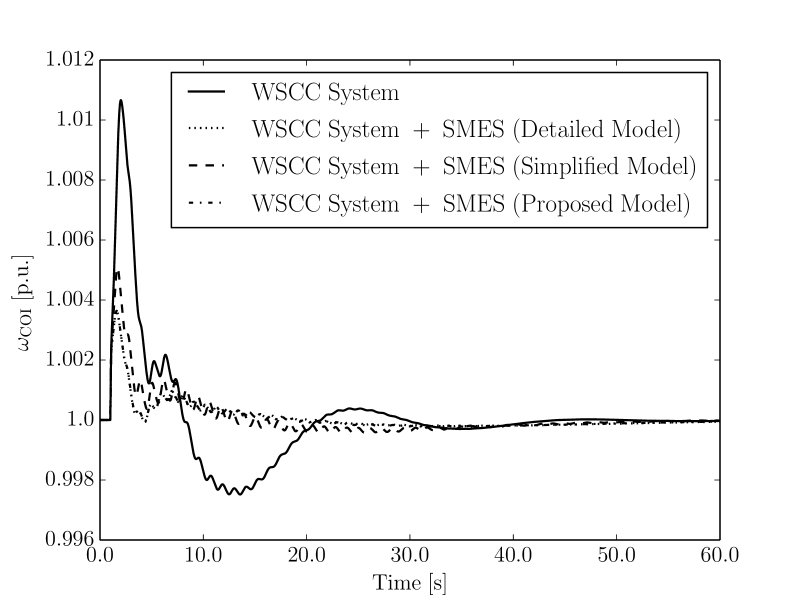
(b)

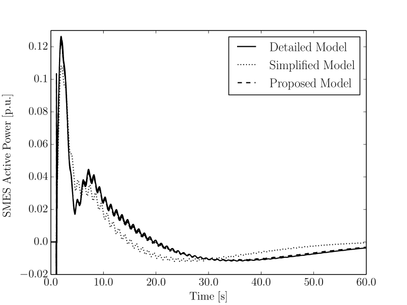
(c)

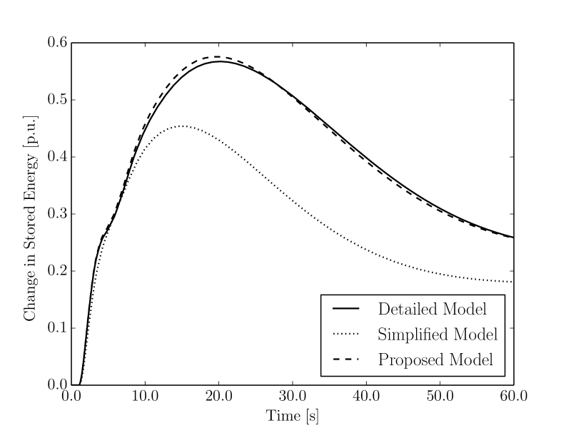
Figure 12: Response of the WSCC system with a SMES following a three-phase fault at bus 7. (a) Frequency of the COI. (b) Active power of the SMES. (c) Change in the Stored Energy of the SMES.

(a)

(b)

(c)

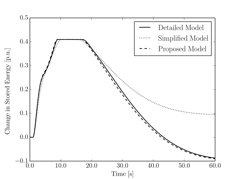
Figure 13: Response of the WSCC system following a three-phase fault at bus 7 when the SMES reaches its maximum storable energy. (a) Frequency of the COI. (b) Active power of the SMES. (c) Change in the Stored Energy of the SMES.

(a)

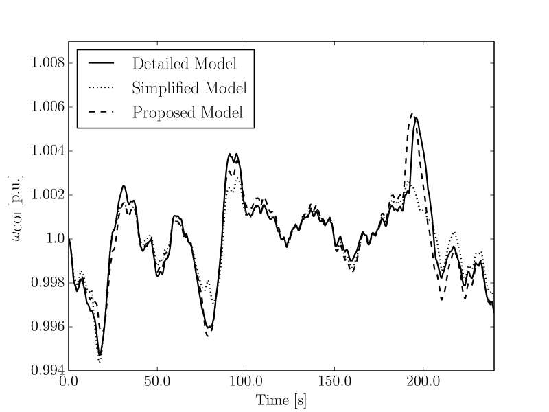
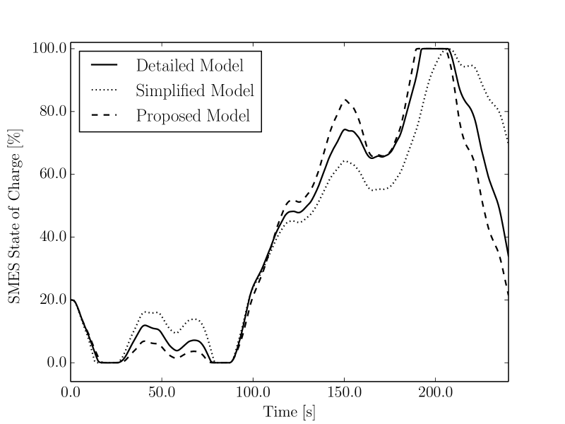
(b)

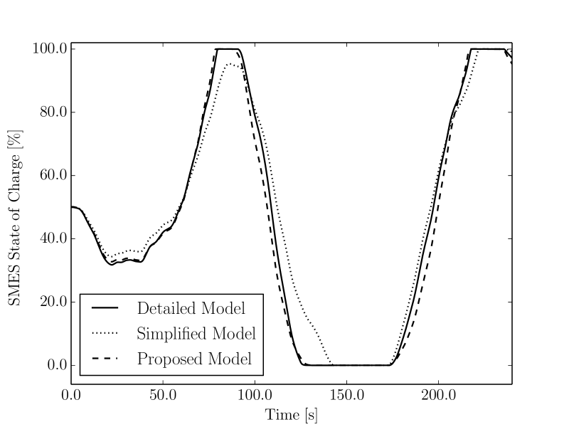
(c)

Figure 14: Response of the WSCC system with a SMES considering stochastic variations of the loads. (a) The initial state of charge of the SMES is 20%. (b) The initial state of charge of the SMES is 50%. (c) The initial state of charge of the SMES is 80%.

IV-A SMES

In this subsection, the storage device connected to bus 8 is a $15$ MW, $60$ MJ SMES, whose model is described in Subsection III-B. To the best of our knowledge, the largest installed SMES (Center of Advanced Power Systems, Florida State University) has a capacity of $100$ MJ, and can provide $100$ MW peak and $\pm 50$ MW oscillatory power [10]. Two scenarios have been considered: Subsection IV-A1 compares the dynamic response of the models of the SMES when the system faces a three-phase fault, whereas Subsection IV-A2 considers stochastic variations of the loads and different initial states of charge of the SMES.

IV-A1 Contingency

A three-phase fault occurs at bus 7 at $t=1$ s and is cleared after $70$ ms through the disconnection of the line which connects buses 7 and 5. In this case, the frequency of the center of inertia (COI) of the system is regulated and its trajectory is shown in Fig. 12 using the detailed and the proposed models of the SMES. Figure 12 also shows the frequency of the COI when the SMES is modeled using the simplified model described in Subsection II-B.

It can be observed that without ESS, the frequency variation after the fault is around $1\%$, and the steady-state is reached after about $40$ s. The inclusion of the SMES in the system allows reducing the overshoot by $60\%$. Moreover, the settling time is about $15$ s.

Figure 12 compares the active power output of the SMES when the detailed and the proposed models are used. The SMES uses the load notation, therefore positive values of the power indicate that the SMES is storing energy, and vice versa.

Finally, Fig. 12 depicts the variation of the energy stored in the SMES. The base of the energy is 100 MJ, therefore the SMES increases its stored energy a maximum of about $57$ MJ during and after the fault. The steady state value of the energy after the occurrence of the disturbance is about $20$ MJ over the initial conditions. As it can be observed from Fig. 12, the performance of the system is basically the same when using the detailed and the proposed models of the SMES.

Figure 13 shows the performance of the system when the SMES reaches its maximum storable energy. In this simulation, it has been considered a maximum variation in the energy of $40$ MJ over the initial condition. It can be observed that the effect of this sort of non-linearity is precisely captured by the proposed model, and the differences in the performance between the detailed and the proposed models are very small.

Figures 12 and 13 also show the transient response of the SMES when the commonly-used simplified model of ESSs described in Subsection II-B is applied. Gains and time constants of the different controllers defined in Section II have the same value for all ESS models. The trajectories obtained by imposing the simplified model consistently deviate from the behavior of the detailed one, particularly after the transient and after reaching the maximum variation of stored energy (note that, for a fair comparison, energy limits are also included in the simplified model in Fig. 13). The proposed generalized model is able to accurately track the behavior of the detailed one in both, fast (transient) and slow (post-contingency) dynamics. On the other hand, the simplified model is accurate only in the first few seconds after the disturbance. The poor performance of the simplified model is an expected consequence of the reduced order of its dynamic equations.

IV-A2 Stochastic Load Variations

In this scenario, all loads are modeled considering stochastic variations of the power consumptions. The Ornstein-Uhlenbeck’s process, also known as mean-reverting process, is used to model such variations [33, 34]. The step size of the Wiener’s process is $h=0.01$s, and the time step of the time integration $\Delta t$ is set to $0.1$s. Initial values of the load and generation are set using a uniform distribution with 5% of variation with respect to the base-case.

Figure 14 shows the frequency of the COI and the state of charge of the SMES for three different load profiles and for an initial state of charge of 20%, 50%, and 80% in Figs. 14, 14, and 14, respectively. These percentages are expressed in terms of the allowed energy variability of the storage device. For each simulation, SMES models are simulated considering same load variation profiles.

The following remarks are relevant:

• The proposed generalized ESS model tracks the behavior of the detailed one better than the commonly-used simplified model of the SMES, for any initial state of charge.

• The proposed model is more accurate the closer is the state of charge to the initial condition during the simulations. This is an expected property of linearized models.

• Based on the results of hundreds of simulations with different load profiles and initial conditions, it has been observed that the best average accuracy of the proposed generalized model is obtained by computing the matrices of (12)-(13) for an initial state of charge of 50%.

IV-B CAES

In this case study, we consider a $15$ MW, $30$ bar CAES, whose model is described in Subsection III-C. The CAES regulates the active power flowing through the transformer connecting buses 2 and 7. As in previous Subsection, the CAES uses the load notation, and two scenarios are performed: Subsection IV-B1 considers a loss of load as contingency, while Subsection IV-B2 includes stochastic variations in all loads. Note that the maximum size of currently installed above-ground CAESs is up to $5$ MW [1]. In this example, we assume that the CAES has three times this capacity.

IV-B1 Contingency

The contingency is a loss of load of $15$ MW occurring at bus 5 at $t=10$ s. Finally, the load is reconnected at $t=80$ s. Figures 15 and 15 illustrate the active power flowing through the transformer connecting buses 2 and 7 and the active power of the CAES, respectively. It can be seen that the response of the CAES simulated using the proposed model is accurate despite the complexity of the detailed CAES model shown in Subsection III-C.

(a)

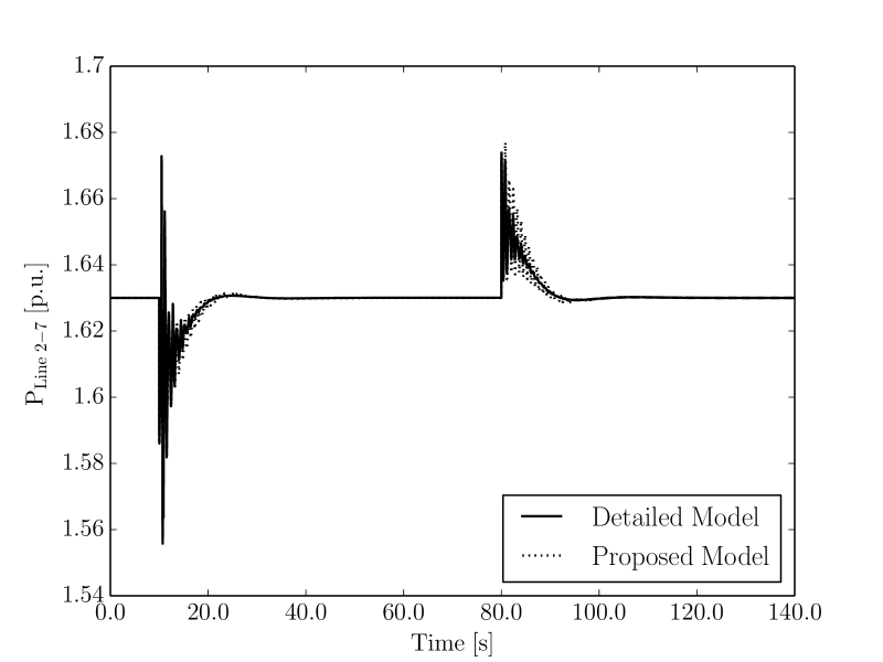
(b)

Figure 15: Response of the WSCC system with a CAES following a loss of load. (a) Power flowing through the transformer connecting buses 2 and 7. (b) Active power of the CAES.

(a)

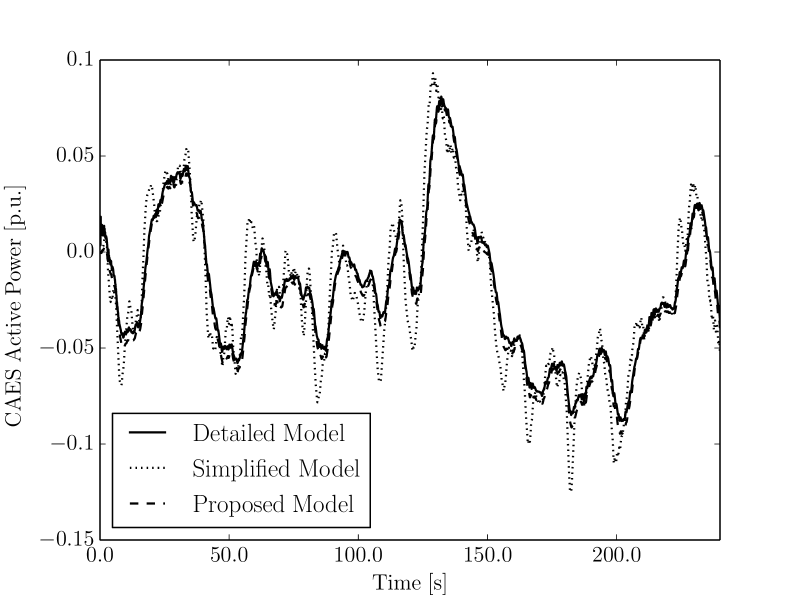
(b)

Figure 16: Response of the WSCC system with a CAES considering stochastic perturbations in the loads. (a) Same control parameters for all models. (b) Control parameters of the simplified CAES model are three times smaller than those of the detailed and the generalized ones.

IV-B2 Stochastic Load Variations

In this scenario, all loads are modeled using the mean-reverting process, (see Subsection IV-A2). Figure 16 depicts the active power of the CAES for each model of this device, for an initial state of charge of about 50%. All control parameters are the same for all models. The time constants of the simplified model of the CAES have been tuned after several trial and error attempts, in order to obtain the behavior as close as possible to the detailed model. Figure 16 shows that the response of the commonly-used simplified model differs considerably from the one of the detailed model. On the other hand, the proposed generalized model appears to be very accurate. In order to obtain a more accurate response of the storage device using the simplified model, it is required to properly tune the control gains $K_{\rm p\it P}$ and $K_{\rm i\it P}$ of the controller depicted in Fig. 7. Figure 16 depicts the response of the CAES considering the same load profiles as in Fig. 16, and when the gains $K_{\rm p\it P}$ and $K_{\rm i\it P}$ are three times smaller than the gains $K_{\rm pu}$ and $K_{\rm iu}$ of the storage controller of Fig. 6, respectively. Some remarks can be deduced:

• The accuracy of the proposed generalized model does not appear to be affected by the complexity and the size of order reduction of the original detailed model. Note that the order reduction achieved in the case of the CAES is from 29 variables in the detailed model to only 5 in the proposed one.

• The accuracy of the commonly-used simplified model cannot be guaranteed even if a lengthy and careful tuning of its control parameters is carried out.

• Because of the required tuning, the design of control strategies cannot be based on the simplified model. On the other hand, exactly same control parameters can be used for both the generalized and detailed ESS models.

IV-C BES

In this example, a $40$ MW BES is installed at bus 8 [13]. The data of the BES is taken from [35], that describes a $55$ MW, $76.7$ GJ BES used for frequency control. The contingency is a loss of a $40$ MW load at bus 5. The load is disconnected at $t=10$ s, and is reconnected at $t=100$ s. In this case study, the BES regulates the frequency of the COI.

Figures 17 and 17 show the frequency of the COI and the power output of the BES, respectively. The initial SOC of the battery is set to $85\%$ to force operating close to the nonlinear voltage-current characteristic of the battery [12, 13]. As stated in Subsection III-D, two sets of matrices for the general model of the BES have to be considered because of the discontinuity in the polarization voltage, $v_{\rm p}$, depending on whether the battery is charging (time from $t=10$ s to $t=100$ s) or discharging (time from $t=100$ s). It can be seen from Fig. 17 that the generalized model is able to track, with a good level of accuracy, the behavior of the detailed model of the BES for both operating conditions, despite the nonlinearities of the device at such a high initial SOC, and the switching between the two operating modes.

(a)

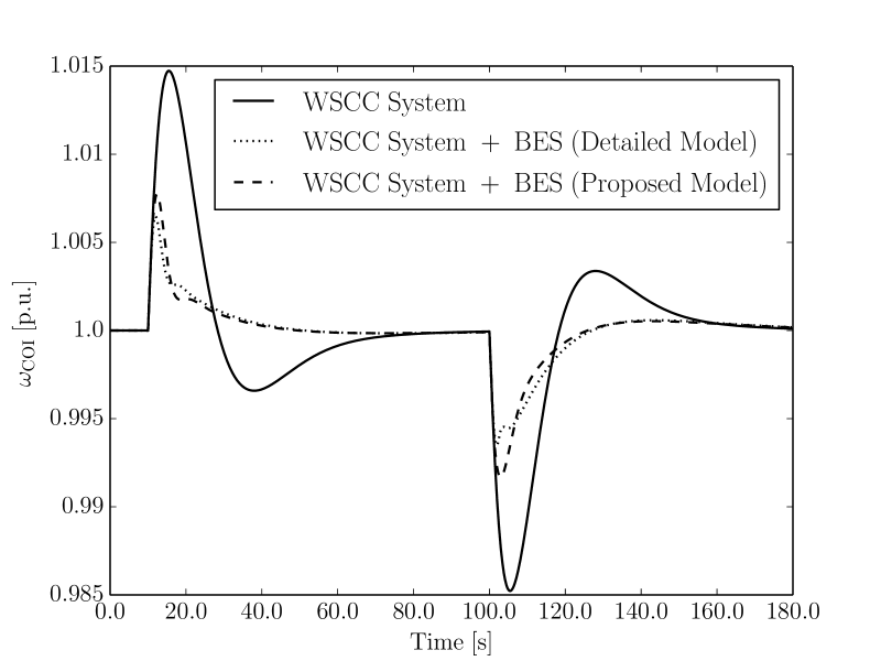
(b)

Figure 17: Response of the WSCC system with a BES following a loss of load. (a) Frequency of the COI. (b) Active power of the BES.

IV-D Concluding Remarks

The following remarks on the proposed generalized model of ESSs are relevant.

1. The proposed model provides a good compromise between simplicity and accuracy. In fact, the proposed model has a reduced and constant dynamic order but, nevertheless it can reproduce faithfully the behavior of ESSs whose detailed transient stability models are considerably more complex (e.g., CAES). On the contrary, the case study shows that simpler models of ESSs might not be precise, particularly if windup limiters are binding.

2. Linearization of a subset of ESS equations does not affect accuracy. The rationale behind this observation is that most ESS variables involved in nonlinear equations are bounded and, hence, the ESS operating point does not vary consistently even after a large perturbation.

3. Detailed ESS models are needed to define the parameters of the proposed model. These data have to be provided by ESS manufactures, in the same way makers provide $d$- and $q$-axis reactances and time constants of the synchronous machine Park model. Hence, we consider that the proposed ESS model can be an opportunity to define a ESS standard for transient stability analysis.

4. Control strategies designed for the proposed generalized model can be directly applied to the detailed ESS models. The linear structure of the equations of the proposed model simplifies the design of more advanced and robust control strategies for ESSs that could be applied subsequently to the detailed models of these devices.

V Conclusions

This paper proposes a generalized model of energy storage devices for voltage and angle stability analysis. Such a model allows simulating different technologies using a fixed set of DAEs and parameters. Simulation results show that the proposed model is able to accurately reproduce the dynamic behavior of detailed transient stability models for large disturbances, namely faults and loss of loads, and across their whole operating cycle. The non-linearity of ESS controllers, i.e., hard limits, are also properly taken into account by the proposed model.

The proposed generalized ESS model appears to be particularly useful to synthesize and compare different control strategies. In fact, since the proposed model is composed of a fixed set of equations, the same control scheme can be straightforwardly used for testing the dynamic response of different technologies. This will be addressed in future work.

Álvaro Ortega (S’14) received from Escuela Superior de Ingenieros Industriales, University of Castilla-La Mancha, Ciudad Real, Spain, the degree in Industrial Engineering in 2013, with a final project on modeling and dynamic analysis of compressed air energy storage systems. Since September 2013, he is a Ph.D. student candidate with the Electricity Research Centre, University College Dublin, Ireland.

Federico Milano (SM’09) received from the University of Genoa, Italy, the Electrical Engineering degree and the Ph.D. degree in 1999 and 2003, respectively. From 2001 to 2002 he was with the University of Waterloo, Canada, as a Visiting Scholar. From 2003 to 2013, he was with the University of Castilla-La Mancha, Ciudad Real, Spain. In 2013, he joined the University College Dublin, Ireland, where he is currently an associate professor. His research interests include power system modeling, stability and control.

References

- [1] H. Ibrahim, A. Ilinca, and J. Perron, “Energy Storage Systems - Characteristics and Comparisons,” Renewable and Sustainable Energy Reviews, vol. 12, pp. 1221–1250, 2008.
- [2] M. Beaudin, H. Zareipour, A. Schellenberglabe, and W. Rosehart, “Energy storage for mitigating the variability of renewable electricity sources: An updated review,” Energy for Sustainable Development, vol. 14, pp. 302–313, 2010.
- [3] “Electrical Energy Storage,” white paper, IEC, Dec. 2011.
- [4] A. S. A. Awad, J. D. Fuller, T. H. M. EL-Fouly, and M. M. A. Salama, “Impact of Energy Storage Systems on Electricity Market Equilibrium,” IEEE Transactions on Sustainable Energy, vol. 5, no. 3, pp. 875–885, July 2014.
- [5] L. Xie, A. A. Thatte, and Y. Gu, “Multi-time-scale Modeling and Analysis of Energy Storage in Power System Operations,” in Energytech, 2011 IEEE, Cleveland, OH, May 2011, pp. 1–6.
- [6] F. A. Inthamoussou, J. Pegueroles-Queralt, and F. D. Bianchi, “Control of a Supercapacitor Energy Storage System for Microgrid Applications,” IEEE Transactions on Energy Conversion, vol. 28, no. 3, pp. 690–697, Sept. 2013.
- [7] IEEE Task Force on Benchmark Models for Digital Simulation of FACTS and Custom-Power Controllers, T&D Committee, “Detailed Modeling of Superconducting Magnetic Energy Storage (SMES) System,” IEEE Transactions on Power Delivery, vol. 21, no. 2, pp. 699–710, Apr. 2006.
- [8] M. H. Ali, B. Wu, and R. A. Dougal, “An Overview of SMES Applications in Power and Energy Systems,” IEEE Transactions on Sustainable Energy, vol. 1, no. 1, pp. 38–47, Apr. 2010.
- [9] F. Milano and R. Zárate Miñano, “Study of the Interaction between Wind Power Plants and SMES Systems,” in 12th Wind Integration Workshop, London, UK, Oct. 2013.
- [10] C. A. Luongo, T. Baldwin, P. Ribeiro, and C. M. Weber, “A 100 MJ SMES Demonstration at FSU-CAPS,” IEEE Transactions on Applied Superconductivity, vol. 13, no. 2, pp. 1800–1805, June 2003.
- [11] V. Vongmanee, “The Renewable Energy Applications for Uninterruptible Power Supply Based on Compressed Air Energy Storage System,” in IEEE Symposium on Industrial Electronics and Applications (ISIEA 2009), Kuala Lumpur, Malaysia, Oct. 2009, pp. 827–830.
- [12] O. Tremblay, L.-A. Dessaint, and A.-I. Dekkiche, “A Generic Battery Model for the Dynamic Simulation of Hybrid Electric Vehicles,” in Vehicle Power and Propulsion Conference. Arlington, TX: IEEE, 2007, pp. 284–289.
- [13] C. M. Shepherd, “Design of Primary and Secondary Cells II. An Equation Describing Battery Discharge,” Journal of the Electrochemical Society, vol. 112, no. 7, pp. 657–664, 1965.
- [14] S. Samineni, B. K. Johnson, H. L. Hess, and J. D. Law, “Modeling and Analysis of a Flywheel Energy Storage System for Voltage Sag Correction,” IEEE Transactions on Industry Applications, vol. 42, no. 1, pp. 42–52, Jan. 2006.
- [15] G. Li, S. Cheng, J. Wen, Y. Pan, and J. Ma, “Power System Stability Enhancement by a Double-fed Induction Machine with a Flywheel Energy Storage System,” in Power Engineering Society General Meeting, IEEE, Montreal, Que, 2006.
- [16] B. C. Pal, A. H. Coonick, I. M. Jaimoukha, and H. El-Zobaidi, “A Linear Matrix Inequality Approach to Robust Damping Control Design in Power Systems with Superconducting Magnetic Energy Storage Device,” IEEE Transactions on Power Systems, vol. 15, no. 1, pp. 356–362, Feb. 2000.
- [17] J. Wu, J. Wen, H. Sun, and S. Cheng, “Feasibility Study of Segmenting Large Power System Interconnections With AC Link Using Energy Storage Technology,” IEEE Transactions on Power Systems, vol. 27, no. 3, pp. 1245–1252, Aug. 2012.
- [18] X. Sui, Y. Tang, H. He, and J. Wen, “Energy-Storage-Based Low-Frequency Oscillation Damping Control Using Particle Swarm Optimization and Heuristic Dynamic Programming,” IEEE Transactions on Power Systems, Mar. 2014.
- [19] V. P. Singh, S. R. Mohanty, N. Kishor, and P. K. Ray, “Robust H-infinity load frequency control in hybrid distributed generation system,” Electrical Power & Energy Systems, vol. 46, pp. 294–305, 2013.
- [20] J. Fang, W. Yao, Z. Chen, J. Wen, and S. Cheng, “Design of Anti-Windup Compensator for Energy Storage-Based Damping Controller to Enhance Power System Stability,” IEEE Transactions on Power Systems, vol. 29, no. 3, pp. 1175–1185, May 2014.
- [21] N. R. Chaudhuri, B. Chauduri, R. Majumder, and A. Yazdani, Multi-terminal Direct-current Grids: Modeling, Analysis, and Control. John Wiley & Sons, 2014.
- [22] J. Beerten, S. Cole, and R. Belmans, “Modeling of Multi-Terminal VSC HVDC Systems With Distributed DC Voltage Control,” IEEE Transactions on Power Systems, vol. 29, no. 1, pp. 34–42, Jan. 2014.
- [23] N. R. Chaudhuri, R. Majumder, B. Chauduri, and J. Pan, “Stability Analysis of VSC MTDC Grids Connected to Multimachine AC Systems,” IEEE Transactions on Power Delivery, vol. 26, no. 4, pp. 2774–2784, Oct. 2011.
- [24] S. Cole, “Steady-State and Dynamic Modelling of VSC HVDC Systems for Power System Simulation,” Ph.D. dissertation, Katholieke Universiteit Leuven, Sept. 2010.
- [25] E. Acha and B. Kazemtabrizi, “A New STATCOM Model for Power Flows Using the Newton–Raphson Method,” IEEE Transactions on Power Systems, vol. 28, no. 3, pp. 2455–2465, Aug. 2013.
- [26] Á. Ortega and F. Milano, “Design of a Control Limiter to Improve the Dynamic Response of Energy Storage Systems,” in Power Engineering Society General Meeting, IEEE, Denver, Colorado, USA, July 2015.
- [27] P. Aristidou, D. Fabozzi, and T. V. Cutsem, “Dynamic Simulation of Large-Scale Power Systems Using a Parallel Schur-Complement-Based Decomposition Method,” IEEE Transactions on Parallel and Distributed Systems, vol. 25, no. 10, pp. 2561–2570, Oct. 2014.
- [28] P. C. Krause, O. Wasynczuk, and S. D. Sudhoff, Analysis of Electric Machinery and Drive Systems, 2nd ed. Wiley-IEEE Press, 2002.
- [29] A. Esmaili, B. Novakovic, A. Nasiri, and O. Abdel-Baqi, “A Hybrid System of Li-Ion Capacitors and Flow Battery for Dynamic Wind Energy Support,” IEEE Transactions on Industry Applications, vol. 49, no. 4, pp. 1649–1657, Aug. 2013.
- [30] P. M. Anderson and A. A. Fouad, Power System Control and Stability, 2nd ed. Wiley-IEEE Press, 2003.
- [31] Illinois Center for a Smarter Electric Grid (ICSEG), “WSCC 9-Bus System,” URL: http://publish.illinois.edu/smartergrid/wscc-9-bus-system/.
- [32] F. Milano, “A Python-based Software Tool for Power System Analysis,” in Procs. of the IEEE PES General Meeting, Vancouver, BC, July 2013.
- [33] M. Perninge, V. Knazkins, M. Amelin, and L. Söder, “Risk Estimation of Critical Time to Voltage Instability Induced by Saddle-Node Bifurcation,” IEEE Transactions on Power Systems, vol. 25, no. 3, pp. 1600–1610, Aug. 2010.
- [34] F. Milano and R. Zárate Miñano, “A Systematic Method to Model Power Systems as Stochastic Differential Algebraic Equations,” IEEE Transactions on Power Systems, vol. 28, no. 4, pp. 4537–4544, June 2013.
- [35] P. Mercier, R. Cherkaoui, and A. Oudalov, “Optimizing a Battery Energy Storage System for Frequency Control Application in an Isolated Power System,” IEEE Transactions on Power Systems, vol. 24, no. 3, pp. 1469–1477, Aug. 2009.