Local Radiation Hydrodynamic Simulations of Massive Star Envelopes at the Iron Opacity Peak

Abstract

We perform three dimensional radiation hydrodynamic simulations of the structure and dynamics of radiation dominated envelopes of massive stars at the location of the iron opacity peak. One dimensional hydrostatic calculations predict an unstable density inversion at this location, whereas our simulations reveal a complex interplay of convective and radiative transport whose behavior depends on the ratio of the photon diffusion time to the dynamical time. The latter is set by the ratio of the optical depth per pressure scale height, $\tau_{0}$, to $\tau_{c}=c/c_{g}$, where $c_{g}\approx 50\ {\rm km\ s^{-1}}$ is the isothermal sound speed in the gas alone. When $\tau_{0}\gg\tau_{c}$, convection reduces the radiation acceleration and removes the density inversion. The turbulent energy transport in the simulations agrees with mixing length theory and provides its first numerical calibration in the radiation dominated regime. When $\tau_{0}\ll\tau_{c}$, convection becomes inefficient and the turbulent energy transport is negligible. The turbulent velocities exceed $c_{g}$, driving shocks and large density fluctuations that allow photons to preferentially diffuse out through low-density regions. However, the effective radiation acceleration is still larger than the gravitational acceleration so that the time average density profile contains a modest density inversion. In addition, the simulated envelope undergoes large-scale oscillations with periods of a few hours. The turbulent velocity field may affect the broadening of spectral lines and therefore stellar rotation measurements in massive stars, while the time variable outer atmosphere could lead to variations in their mass loss and stellar radius.

1. Introduction

Massive stars play an important role in many astrophysical environments. The radiative and mechanical energy output from massive stars are important feedback mechanisms regulating star formation and the structure of the interstellar medium in galaxies (Kennicutt, 2005; Smith, 2014). Radiation from massive stars also plays an important role in the reionization of the universe (Bromm & Larson, 2004). When massive stars explode, they produce various types of supernovae and high energy transients, while leaving behind black holes and neutron stars whose properties depend on the previous history of massive stellar evolution (Heger et al., 2003).

Because of the steep mass-luminosity relation of main sequence stars, the luminosity approaches the Eddington-limit for electron scattering in stars with masses larger than $\sim 50-100M_{\odot}$ (Crowther, 2007; Maeder et al., 2012; Sanyal et al., 2015). In massive star envelopes with non-zero metallicity, the opacity increases significantly compared with electron scattering due to iron opacity at temperatures $\approx 1.8\times 10^{5}$ K (e.g., Paxton et al. 2013 and references therein). As a result, the actual radiation force can locally exceed the gravitational force near the iron opacity peak. This same physics can operate at somewhat lower temperatures due to the opacity produced by helium and hydrogen (e.g. Maeder, 1981).

The locally super-Eddington luminosity near the iron opacity peak (and related opacity peaks) has been a long standing challenge for one dimensional (1D) stellar evolution models of massive stars. Hydrostatic and thermal equilibrium models with a super-Eddington luminosity require density and gas pressure inversions (Joss et al., 1973a; Gräfener et al., 2012; Paxton et al., 2013; Owocki, 2015), which are usually convectively unstable. When the iron opacity peak is sufficiently deep in the star, convection is efficient and can rearrange the stellar structure to have constant entropy, removing the density inversion predicted by radiative equilibrium models. When the iron opacity peak is close to the surface, however, convection is inefficient and cannot carry the necessary super-Eddington flux. It is unclear how the stellar structure adjusts in this limit, and in particular if the density inversions are stable (Maeder, 2009; Sanyal et al., 2015). This results in very uncertain stellar radii in the very massive star regime (Yusof et al., 2013; Köhler et al., 2015). To complicate the situation even further, stellar evolution calculations of massive stars become numerically difficult when the opacity near the stellar photosphere significantly exceeds the electron scattering opacity. In this situation the convective energy transport is often artificially enhanced in 1D stellar evolution models (Maeder, 1987; Paxton et al., 2013), which leads to the disappearance of the density inversions (Stothers & Chin, 1979).

The density and temperature dependence of the opacity near composition-specific opacity peaks can also drive radiation hydrodynamic instabilities distinct from convection (Kiriakidis et al., 1993; Blaes & Socrates, 2003; Suárez-Madrigal et al., 2013). In many cases, these cannot be captured by 1D stellar evolution models. These instabilities have been suggested as the origin of the large mass loss rates from massive stars that cannot be explained by line-driven winds (Glatzel & Kiriakidis, 1993). The amount of mass loss by line driven winds (Puls et al., 2008) also depends on the structure of the stellar photosphere (e.g., the amplitude of density and velocity fluctuations, potentially affecting the degree of wind clumping).

In this paper, we present three-dimensional (3D) radiation hydrodynamic simulations of stellar envelopes near the iron opacity peak and quantify the impact of convective and radiation hydrodynamic instabilities on the stellar envelopes’ properties and dynamics. These calculations provide the first direct calibration of classical mixing length theory (MLT) (Cox, 1968) in the radiation pressure dominated regime. In addition, we quantify the extent to which convection and/or other hydrodynamic instabilities generate a “porous” atmosphere that substantially increases the radiation flux relative to that predicted by one-dimensional models. This is critical for determining whether locally super-Eddington regions in a stellar envelope can initiate a large-scale stellar wind via continuum radiation pressure or whether the stellar radiation freely escapes through low density channels (Shaviv, 1998; van Marle et al., 2008).

Our work utilizes numerical techniques for accurate 3D radiation hydrodynamic simulations based on a variable Eddington tensor (VET) formalism (Jiang et al., 2012; Davis et al., 2012). These techniques have been successfully used to study a wide range of astrophysical problems (Jiang et al., 2013a, b, 2014b) and have significant advantages relative to ad-hoc closures such as the flux-limited diffusion (FLD) approximation (Davis et al., 2014; Proga et al., 2014). The direct solution of the radiation transfer equation (via VET or Monte-Carlo methods) is particularly important for studying mildly optically thick regions near the stellar photosphere. Indeed, recent studies have shown that approximate radiation transfer schemes such as FLD or M1 can reach completely opposite conclusions compared with VET or Monte Carlo methods (Davis et al., 2014; Tsang & Milosavljevic, 2015).

The remainder of this paper is organized as follows. In §2 we identify the key dimensionless parameter that governs the physics of near surface convection zones in stellar envelopes. We also describe the 1D stellar models that motivate the specific conditions in our 3D radiation hydrodynamic simulations. In §3 we describe our numerical methods while in §4 we present our results. Finally, in §5 we summarize our key results and discuss their implications.

2. The Model Parameters

The relative importance of convective and radiative energy transport can be characterized by a critical optical depth $\tau_{c}$ over the pressure scale height $H_{0}$ near the iron opacity peak. As we will show based on our simulations, for conditions typical of massive stars, the maximum turbulent velocity reaches the isothermal sound speed when convection starts to become inefficient. Then the critical optical depth can be estimated by balancing the diffusive radiation flux $\sim a_{r}T_{0}^{4}c/\tau$ and the maximal convective flux in the radiation pressure dominated regime $\sim c_{g,0}a_{r}T_{0}^{4}$:

$$\tau_{c}=c/c_{g,0}.$$ (1)

We define the gas isothermal sound speed $c_{g,0}$, radiation sound speed $c_{s,0}$, pressure scale height $H_{0}$, optical depth $\tau_{0}$ and typical dynamic time scale $t_{0}$ based on the density $\rho_{0}$ and temperature $T_{0}$ at the iron opacity peak

$$c_{g,0} = \sqrt{\frac{P_{0}}{\rho_{0}}},$$

$$c_{s,0} = \sqrt{\frac{a_{r}T_{0}^{4}}{3\rho_{0}}},$$

$$H_{0} = \frac{c_{s,0}^{2}}{g}=\frac{a_{r}T_{0}^{4}}{3\rho_{0}g},$$

$$\tau_{0} = \kappa_{t}(\rho_{0},T_{0})\rho_{0}H_{0},$$

$$t_{0} = \frac{H_{0}}{c_{s,0}}.$$ (2)

The characteristic radiation pressure is $P_{r,0}=a_{r}T_{0}^{4}/3$ while the gas pressure is $P_{0}$.

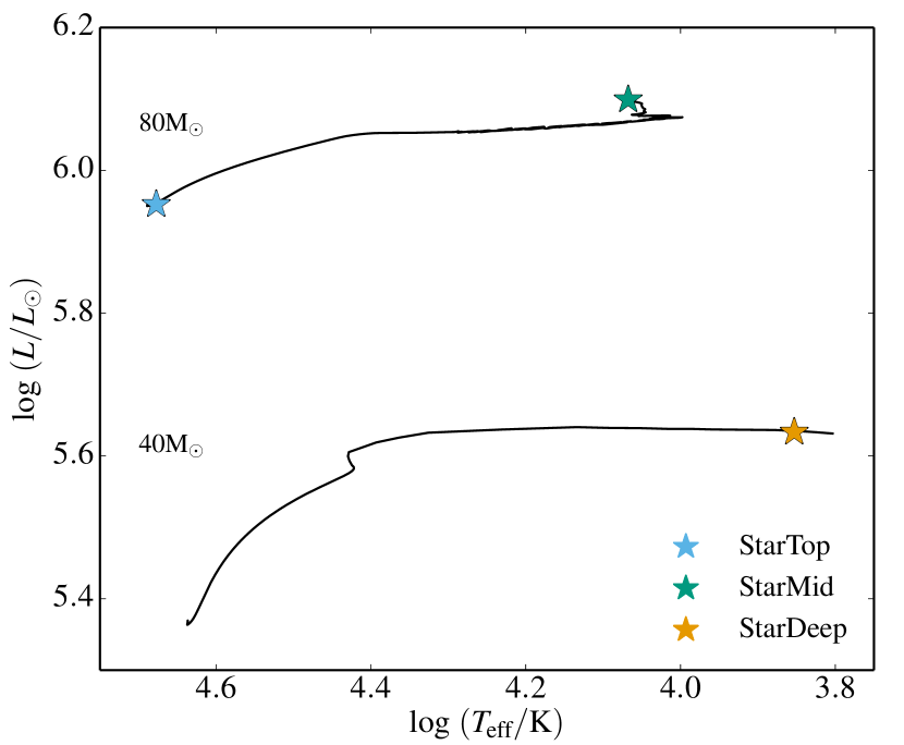
Figure 1.— Stellar evolution tracks of two solar metallicity stars with initial mass of $40M_{\odot}$ and $80M_{\odot}$ calculated with the 1D stellar evolution code MESA. The stellar symbols identify the locations corresponding to the three initial conditions of the 3D radiation hydro calculations with Athena listed in Table 1. The Athena calculations are effectively local plane-parallel atmosphere calculations motivated by the MESA models.

A related way to interpret the critical optical depth $\tau_{c}$ in equation (1) is that the typical thermal time scale due to photon diffusion $t_{c}$ near the iron opacity peak is given by

$$t_{c}=\frac{\tau_{0}H_{0}}{c}=\frac{\tau_{0}}{\tau_{c}}\frac{c_{s,0}}{c_{g,0}}t_{0}.$$ (3)

When $\tau_{0}\gg\tau_{c}$, the diffusion time scale is longer than the local dynamic time scale and we expect convection to be an efficient energy transport mechanism. When $\tau_{0}\ll\tau_{c}$, however, radiative diffusion is rapid enough that convection may behave very differently compared with classical mixing length theory. This can also be related to the Péclet number $P_{e}$, which is the ratio of advective to diffusive flux. When $\tau_{0}\gg\tau_{c}$, we expect $P_{e}\gtrsim 1$, while when $\tau_{0}\ll\tau_{c}$, $P_{e}\lesssim 1$. Note that there is some ambiguity as to whether $\tau_{c}$ should be defined in terms of the gas isothermal sound speed $c_{g,0}$ or the radiation sound speed $c_{s,0}$. As we shall show, we find that the former better characterizes the maximum velocities reached in our simulations.

In order to identify stellar conditions spanning the different regimes of radiation dominated convection, we use Modules for Experiments in Stellar Evolution (MESA, Paxton et al. (2011, 2013, 2015) release r7385) to evolve stars with initial mass $40M_{\odot}$ and $80M_{\odot}$. The models have an initial metallicity $Z=0.02$ with a mixture taken from Asplund et al. (2005) and are calculated using the OPAL opacity tables (Iglesias & Rogers, 1996). Convection is accounted for using mixing-length theory (MLT) in the Henyey et al. (1965) formulation with $\alpha_{\mathrm{MLT}}=1.5$. Convective boundaries are determined using the Ledoux criterion and we use semiconvection with an efficiency $\alpha_{\mathrm{sc}}$ = 0.01 (Langer et al., 1983, 1985). An exponentially decaying overshooting (Herwig, 2000) has been included with $\alpha_{\mathrm{ov}}=0.001$ above and below convective boundaries. Stellar winds are included according to the mass loss scheme described in Glebbeek et al. (2009) (Dutch wind scheme) with an efficiency parameter $\eta=0.8$.

We have identified specific times in the MESA massive star models with conditions that range from $\tau_{0}/\tau_{c}\ll 1$ to $\tau_{0}/\tau_{c}\gg 1$. We label these models as StarDeep, StarMid and StarTop; they have $\tau_{0}/\tau_{c}=15.2,0.97$ and $0.025$, respectively. Figure 1 shows the positions of these models in the HR diagram. Model StarDeep has an initial mass of $40M_{\odot}$. It is evolved to an age of $4.3\times 10^{6}$ year in MESA at which point it has an effective temperature $7.13\times 10^{3}$ K, radius $431R_{\odot}$ and luminosity $8.96\times 10^{5}L_{\odot}$. Model StarMid starts from a $80M_{\odot}$ star. At an age of $3.02\times 10^{6}$ year it has an effective temperature $1.17\times 10^{4}$ K, radius $274R_{\odot}$ and luminosity $1.26\times 10^{6}L_{\odot}$. Model StarTop also starts from an $80M_{\odot}$ star but is only evolved to an age of $9.15\times 10^{4}$ year, at which point it has an effective temperature $4.75\times 10^{4}$ K, radius $14R_{\odot}$ and luminosity $8.96\times 10^{5}L_{\odot}$.

As described in §3, we use plane-parallel 3D radiation hydrodynamics simulations to study the physics of massive stellar envelopes. The initial radial location of the iron opacity peak $r_{0}$ and the density $\rho_{0}$, temperature $T_{0}$ and luminosity $L_{0}$ at this location are taken from the corresponding MESA models. The fiducial parameters of our initial conditions are listed in Table 1.

3. Numerical Method

3.1. Equations

We model the envelopes of massive stars in plane parallel geometry, neglecting the global stellar geometry. This is suitable for studying the effects of 3D radiation hydrodynamics on energy transport in the stellar envelope, but is not appropriate for studying global effects such as stellar outflows. We solve the frequency-independent (gray) radiation hydrodynamic equations in cartesian coordinates $(x,y,z)$ with unit vectors (${\hat{x}}$, ${\hat{y}}$, ${\hat{z}}$). The gravitational acceleration $g$ is assumed to be a constant and along the $-{\hat{z}}$ direction. As the mass of the envelope is less than $1\%$ of the core mass, this is a reasonable assumption (the slight change in $1/r^{2}$ in the stellar envelope is also neglected). The equations are (e.g., Jiang et al., 2012, 2013a)

$$\frac{\partial\rho}{\partial t}+\nabla\cdot(\rho\bm{v}) = 0,$$

$$\frac{\partial(\rho\bm{v})}{\partial t}+\nabla\cdot({\rho\bm{v}\bm{v}+P{{\sf I}}}) = -{S_{r}}(\bm{P})-\rho g{\hat{z}},\$$

$$\frac{\partial{E}}{\partial t}+\nabla\cdot\left[(E+P)\bm{v}\right] = -cS_{r}(E)-g\rho\bm{v}\cdot{\hat{z}},$$

$$\frac{\partial E_{r}}{\partial t}+\nabla\cdot\bm{F}_{r} = cS_{r}(E),$$

$$\frac{1}{c^{2}}\frac{\partial\bm{F}_{r}}{\partial t}+\nabla\cdot{\sf P}_{r} = {\bf S_{r}}(\bm{P}),$$ (4)

where the radiation source terms are

$${\bf S_{r}}(\bm{P}) = -\rho\left(\kappa_{aF}+\kappa_{sF}\right)\left[\bm{F}_{r}-\left(\bm{v}E_{r}+\bm{v}\cdot{\sf P}_{r}\right)\right]/c$$

$$+ \rho\bm{v}(\kappa_{aP}a_{r}T^{4}-\kappa_{aE}E_{r})/c,$$

$$S_{r}(E) = \rho(\kappa_{aP}a_{r}T^{4}-\kappa_{aE}E_{r})$$ (5)

$$+ \rho(\kappa_{aF}-\kappa_{sF})\frac{\bm{v}}{c^{2}}\cdot\left[\bm{F}_{r}-\left(\bm{v}E_{r}+\bm{v}\cdot{\sf P}_{r}\right)\right].$$

Notice that local thermal equilibrium (LTE) is assumed for the emission term.

In the above equations, $\rho,P,\bm{v},c$ are the gas density, pressure, flow velocity and speed of light respectively. The total gas energy density is $E=E_{g}+\rho v^{2}/2$, where $E_{g}=P/(\gamma-1)$ is the internal gas energy density with a constant adiabatic index $\gamma=5/3$. The gas pressure is $P=\rho\mathrm{k_{B}}T/\mu$, where $\mathrm{k_{B}}$ is Boltzmann’s constant and $\mu=0.62m_{p}$ is the mean molecular weight for nearly fully ionized gas with proton mass $m_{p}$. The radiation constant is $a_{r}=7.57\times 10^{15}$ erg cm^-3 K^-4, while $E_{r},\bm{F}_{r}$ are the radiation energy density and flux. The Rosseland mean absorption and scattering opacities are denoted by $\kappa_{aF}$ and $\kappa_{sF}$, while $\kappa_{aP}$ and $\kappa_{aE}$ are the Planck and energy mean absorption opacities. We describe our choice of these opacities in the following section.

Equations (3.1) and (3.1) are solved in the mixed frame, meaning that the radiation flux $\bm{F}_{r}$ and energy density $E_{r}$ are Eulerian variables, while the material-radiation interaction terms in equations (3.1) are written in the co-moving frame (e.g., Lowrie et al., 1999). The Eulerian and co-moving flux $\bm{F}_{r,0}$ are related through $\bm{F}_{r,0}=\bm{F}_{r}-\left(\bm{v}E_{r}+\bm{v}\cdot{\sf P}_{r}\right)$. Notice that only the co-moving radiation flux contributes to the radiation acceleration while the advection flux does not.

We relate the radiation pressure ${\sf P}_{r}$ and radiation energy density through a variable Eddington tensor (VET), ${\sf P}_{r}={\sf\bm{f}}E_{r}$. We do not use an assumed closure relation (such as FLD or M1) to specify ${\sf\bm{f}}$. Instead, we compute it directly from angular quadratures of the specific intensity $I_{r}$ for each angle $\bm{n}$, which is calculated from the time-independent radiation transfer equation

$$\frac{\partial I_{r}}{\partial s}=\kappa_{t}\left(S-I_{r}\right),$$ (6)

where $S$ is the radiation source term and $\kappa_{t}$ is the total specific opacity. Because the typical dynamic time scale is much longer than the light crossing time, ${\sf\bm{f}}$ barely changes between each time step. Our use of the time independent transfer equation to calculate the angular distribution of the radiation field is thus very accurate. We solve the transfer equation in equation (6) using the method of short characteristics, as described in Davis et al. (2012). Then ${\sf\bm{f}}$ is calculated according to its definition

$${\sf\bm{f}}=\frac{\int I_{r}\bm{n}\bm{n}d\Omega}{\int I_{r}d\Omega},$$ (7)

where $\Omega$ is the solid angle. We emphasize that we only use the time-independent transfer equation (6) to calculate the Eddington tensor ${\sf\bm{f}}$, which represents the angular distribution of the radiation field. The moments of $I_{r}$ are not used to calculate the radiation-material interactions. Instead, the radiation moments $E_{r}$, $\bm{F}_{r}$ and the radiation source terms are calculated self-consistently through the time dependent radiation moment equations (3.1).

The Eddington tensor in equation (7) closes the radiation moment equations (eqs. 3.1). We solve these equations using the Godunov radiation MHD code Athena, as described and tested in Jiang et al. (2012) (and with additional improvements described in Jiang et al. (2013c)). We solve the radiation subsystems as well as the radiation source terms implicitly, while the hydro equations are solved explicitly as in the original Athena code (Stone et al., 2008), with appropriate modifications due to the stiff radiation source terms (Jiang et al., 2012).

3.2. The Opacity

In order to correctly capture the temperature and density dependencies of the opacity, particularly near the iron opacity peak, we directly use the opacity table from MESA (Paxton et al., 2011, 2013, 2015) in our Athena simulations. We assume a metallicity $Z=0.02$ and hydrogen fraction $X=0.6$. For the density $\rho$ and temperature $T$ in each cell, the total specific opacity $\kappa_{t}$ is calculated with bilinear interpolation based on the table. This is used as the total specific flux mean opacity $\kappa_{t}=\kappa_{aF}+\kappa_{sF}$. In order to split this into scattering and absorption opacities, we assume a constant electron scattering opacity $\kappa_{sF}=0.32$ g^-1 cm². All of the absorption opacities ($\kappa_{aF},\kappa_{aP},\kappa_{aE}$) are assumed to be the same for simplicity.

Figure 2.— The opacity $\kappa_{t}$ as a function of density and temperature near the iron opacity peak at $T\approx 1.5\times 10^{5}$ K. Each line shows the opacity as a function of temperature for a fixed density. From top to bottom, the density decreases by a factor of $10$ between neighboring lines.

Figure 2 shows the actual opacity $\kappa_{t}$ we use for a range of temperatures and densities appropriate to stellar envelopes. The opacity peak between $10^{5}$ and $2\times 10^{5}$ K is due to Fe, which is the region we focus on. The increase in opacity at lower temperatures is due to He and H. The iron opacity peak has a sensitive dependence on temperature but a weak dependence on density. Particularly when $\rho\lesssim 3.6\times 10^{-11}$ g cm^-3, $\kappa_{t}$ does not depend on density for $T\gtrsim 10^{5}$ K. For the stellar envelopes we study, the temperature usually does not drop below $4\times 10^{4}$ K. Moreover, when this does happen, the density is always smaller than $10^{-10}$ g/cm³. As a result, the He and H opacity peaks usually do not show up in our calculations.

3.3. Initial and Boundary Conditions

We set our initial conditions in the Athena simulations by using the MESA models described in §2 to determine the initial radial location $r_{0}$, density $\rho_{0}$ and temperature $T_{0}$ at the iron opacity peak. The gravitational acceleration $g$ is also chosen to be the value at $r_{0}$ in the MESA models. We then apply a constant radiation flux $F_{r,i}$ through the whole simulation box, which represents the radiation coming from the center of the massive star. The initial radiation flux is determined by the total luminosity $L_{0}$ in the MESA models at $r_{0}$: $F_{r,i}=L_{0}/(4\pi r_{0}^{2})$.

With these fiducial parameters and the opacity given in §3.2, we construct our initial conditions by solving for a hydrostatic envelope in thermal equilibrium. Starting from $z=r_{0}$, all the fluid and radiation quantities are integrated as a function of height using

$$\frac{\partial P}{\partial z} = \frac{\rho\kappa_{t}}{c}F_{r,i}-\rho g,$$

$$E_{r} = a_{r}T^{4},$$

$$\frac{1}{3}\frac{\partial E_{r}}{\partial z} = -\frac{\rho\kappa_{t}}{c}F_{r,i}.$$ (8)

We integrate above and below $r_{0}$ to capture the whole profile of the iron opacity peak region in our simulation box. We then add random perturbations with $0.01\%$ amplitude to the density in the simulation box of dimensions $L_{x},L_{y},L_{z}$. The initial conditions constructed in this way are slightly different from the 1D profiles returned by MESA models around the iron opacity peak. We only guarantee that the characteristic physical parameters we choose are consistent with the MESA stellar models. In particular, our initial condition does not have any mixing length model of convective or advective energy transport. We then calculate how the energy will be transported using self-consistent 3D radiation hydrodynamic simulations.

At the bottom of the box, we use a reflecting boundary condition for gas quantities. This means that the density, opacity and the horizontal components of the velocity are copied from the last active zones to the ghost zones used for boundary conditions. The vertical component of velocity in the ghost zones is set to be the opposite of the velocity in the last active zones. The radiation flux is fixed at the constant value $F_{r,i}$ while the radiation energy density $E_{r}$ is integrated to the ghost zones using the diffusion equation. For the top boundary, all gas quantities and the radiation flux $\bm{F}_{r}$ are copied from the last active zones to the ghost zones. When the photosphere is included in the simulation box (StarTop & StarMid), the radiation energy density $E_{r}$ in the ghost zones is also copied from the last active zones. When the whole simulation box is optically thick (StarDeep), $E_{r}$ is extended to the ghost zones using the diffusion equation. Periodic boundary conditions are used for all quantities in the horizontal direction.

For the short characteristic module we use to calculate the VET, the incoming specific intensities from the bottom of the domain are chosen such that angular quadratures of the intensities give a constant vertical flux $F_{r,i}$ and the same $E_{r}$ as in the moment equations at the bottom. The incoming specific intensities at the top of the domain are set to zero when the photosphere is inside the simulation box. By contrast, when the whole simulation box is optically thick, the incoming specific intensities from the top of the domain are set to be the same as the outgoing specific intensities.

Table 1Simulation Parameters

Variables/Units	StarDeep	StarMid	StarTop
$r_{0}/R_{\odot}$	125.7	65.6	13.6
$T_{0}$/K	$1.87\times 10^{5}$	$1.67\times 10^{5}$	$1.57\times 10^{5}$
$\rho_{0}$/(g cm-3)	$3.10\times 10^{-8}$	$3.60\times 10^{-9}$	$5.52\times 10^{-9}$
$g$/(cm s-2)	63.59	$3.56\times 10^{2}$	$1.17\times 10^{4}$
$F_{r,i}$/(erg cm-2 s-1)	$1.24\times 10^{12}$	$9.94\times 10^{12}$	$3.06\times 10^{14}$
$H_{0}$/cm	$1.56\times 10^{12}$	$1.52\times 10^{12}$	$2.37\times 10^{10}$
$t_{0}$/s	$1.56\times 10^{5}$	$6.54\times 10^{4}$	$1.42\times 10^{3}$
$\tau_{c}\equiv c/c_{g,0}$	$5.99\times 10^{3}$	$6.62\times 10^{3}$	$6.54\times 10^{3}$
$\tau_{0}$	$9.12\times 10^{4}$	$6.41\times 10^{3}$	$166.5$
$P_{r,0}/P_{0}$	3.96	26.32	13.22
$L_{x,y}/H_{0}$	0.89	0.46	1.17
$L_{z}/H_{0}$	6.26	3.71	4.60
$N_{x,y}$	128	128	128
$N_{z}$	768	1024	512

• Note: The gravitational acceleration $g$ and radiation flux $F_{r,i}$ coming from the bottom of the simulation box are fixed. The optical depth $\tau_{0}$, temperature $T_{0}$, density $\rho_{0}$, radiation and gas pressure $P_{r,0}$, $P_{0}$ are the fiducial parameters for each run. They are also the initial conditions around the iron opacity peak. The number of cells are $N_{x},N_{y}$ and $N_{z}$.

4. Results

4.1. The run StarDeep when $\tau_{0}\gg\tau_{c}$

The run StarDeep is in the regime where the gas and radiation are tightly coupled and we expect efficient convection. Below, we first show how the simulated envelope evolves, then summarize its time averaged structure, and finally compare the energy transport in our 3D radiation hydrodynamic simulation with mixing length theory.

4.1.1 Simulation History

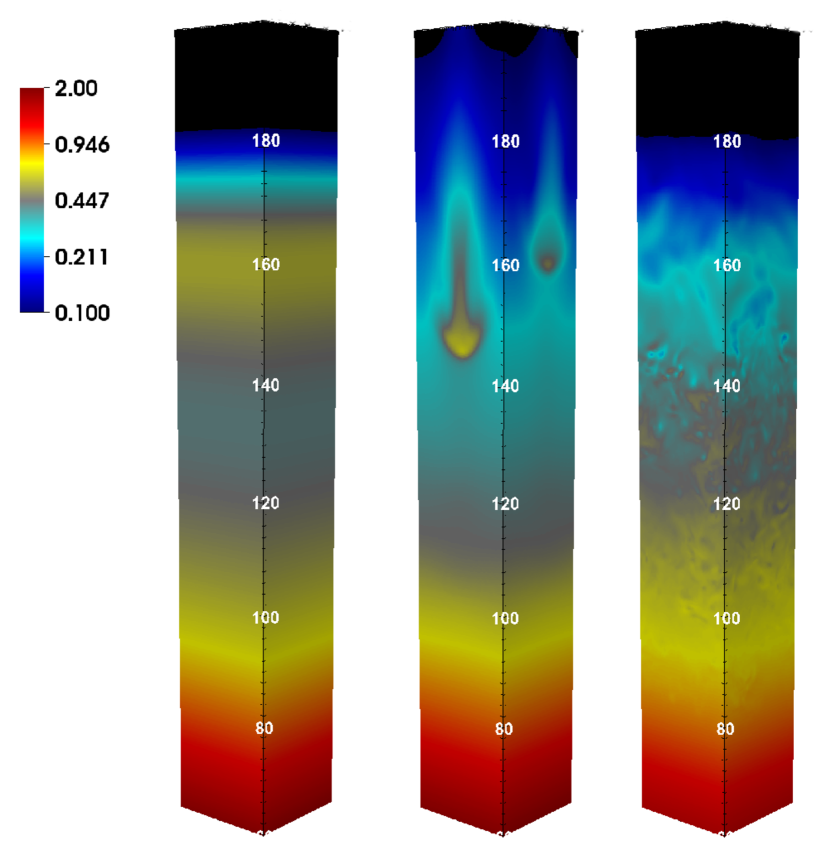
Figure 3.— Snapshots of density for the run StarDeep at time 0 (left), $21.4t_{0}$ (middle) and $97.8t_{0}$ (right). The box sizes labeled in the plots are in units of solar radius $R_{\odot}$. The horizontal box size is $L_{x}=L_{y}=20R_{\odot}$. Density is in units of $\rho_{0}$, which is given in Table 1 for this run.

Three snapshots of density in Figure 3 show the evolution of the envelope. The initial density varies only vertically. At the bottom where the temperature is $30\%$ larger than $T_{0}$, the radiation acceleration is smaller than the gravitational acceleration and both density and temperature decrease with height. Around $z=130R_{\odot}$, where we enter the temperature range of the iron opacity peak, the radiation acceleration becomes larger than the gravitational acceleration for the fixed radiation flux $F_{r,i}$, and the density increases with height, peaking around $z=160R_{\odot}$. Because the temperature always decreases with height according to the diffusion equation, the radiation acceleration eventually decreases after the iron opacity peak. When the radiation flux again becomes sub-Eddington, the density drops with height. The end result is that the initial condition has the density inversion associated with hydrostatic envelopes with a super-Eddington radiation flux (Joss et al., 1973b). This profile is our initial condition for the simulation, and does not represent the profile in the MESA 1D calculation.

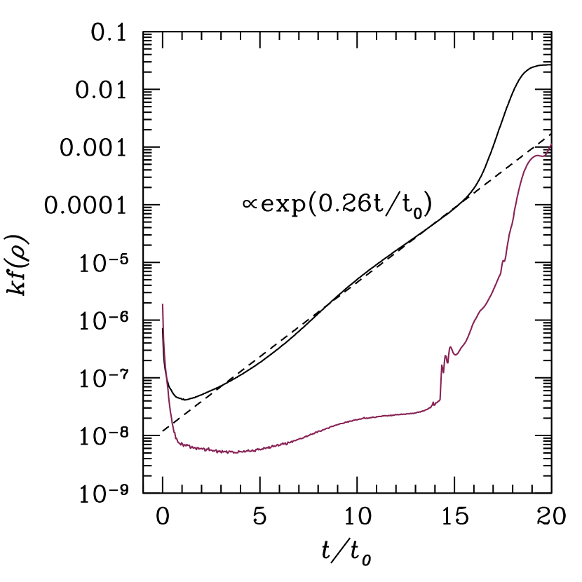
Figure 4.— Time evolution of the density power spectrum $kf(\rho)$ for the run StarDeep at height $z=160R_{\odot}$ during the linear growth phase of convection. The black and red lines are for the modes with wavelength $0.41H_{0}$ and $0.18H_{0}$, respectively. The dashed black line is a fit of an exponential function to the solid black line, which indicates an e-folding time $3.85t_{0}$ for this mode. The power spectrum is normalized by the mean density at $z=160R_{\odot}$, such that the integral of $k^{2}f^{2}(\rho)$ over all wavenumbers is unity.

Figure 5.— History of the radiation energy density weighted ($V_{z,E_{r}}$, solid line) and density weighted ($V_{z,\rho}$, dashed line) vertical velocity for the run StarDeep.

The middle panel of Figure 3 shows that the initial density inversion is unstable. By $t\approx 20t_{0}$, there are large rising and sinking plumes characteristic of convection and/or the Rayleigh-Taylor instability. We now show how this instability can be quantitatively understood as arising from convection in the radiation dominated regime.

The gas and radiation entropy per unit mass $S_{g},S_{r}$ are given by

$$S_{g} \equiv \frac{\mathrm{k_{B}}}{\mu(\gamma-1)}\ln\left[\frac{P/P_{0}}{\left(\rho/\rho_{0}\right)^{\gamma}}\right]\ \ \ {\rm and}$$

$$S_{r} \equiv \frac{4E_{r}}{3\rho T}.$$ (9)

In our simulations, the total entropy is dominated by the radiation. This increases with height near the bottom of the simulation box in the initial condition, but necessarily decreases with height near the density inversion where $T$ decreases but $\rho$ increases (see Fig. 7 discussed below). We thus expect that our initial condition is convectively stable near the bottom of the domain, but convectively unstable near the density inversion region in 3D. This is exactly what we find in the simulation (see Fig. 3). Convection happens around $160R_{\odot}$ within $\approx 20t_{0}$ (equation 3) and mixes the initial density inversion. High density fingers sink and low density gas rises upwards. By $t=97.8t_{0}$ (third panel of Figure 3), the bulk of the stellar envelope has reached a statistically steady turbulent state driven by convection.

The initial radiation Brunt-Väisälä frequency $|N_{r}|$ (e.g. equation 52 of Blaes & Socrates 2003) at the iron opacity peak is $0.8/t_{0}$, but it takes $\approx 20t_{0}$ for convection to begin destroying the initial density inversion. The wavelength of the fastest growing initial mode is about half of the horizontal box size, which also differs from the normal Rayleigh-Taylor instability with a density discontinuity (Jiang et al., 2013a) where the shortest wavelengths grow fastest. To understand the linear growth phase of the instability, we first calculate the 2D discrete Fourier transform in the $x,y$ plane of the density at height $z=160R_{\odot}$ as a function of time. The 2D Fourier coefficient is then binned into a 1D power spectrum $kf(\rho)$, where $k$ is the magnitude of the horizontal wavenumber. The time evolution of two modes with horizontal wavelengths $0.41H_{0}=9.2R_{\odot}$ and $0.18H_{0}=4.0R_{\odot}$ are shown in Figure 4. The decrease of $kf(\rho)$ within $t_{0}$ probably originates from an initial vertical oscillation that is present due to the imperfect balance between gravity and pressure gradients in the initial condition. After this point, the long wavelength mode grows exponentially with an e-folding time $3.85t_{0}$ until $15t_{0}$. The shorter wavelength mode also grows exponentially, but at a rate that is smaller by a factor of $3.44$ initially. However, it then grows quickly after $15t_{0}$ as convection becomes nonlinear and power from long wavelength modes cascades to the short wavelength modes.

The measured growth rates agree very well with the short wavelength WKB linear analysis done by Blaes & Socrates (2003) (the last factor of their equation 59). Plugging in numbers for the long wavelength mode in Figure 4, and assuming that the vertical wavelength of this mode is about equal to its horizontal wavelength, we get a growth rate of $0.27/t_{0}$, very close to the value measured in the simulation. This decline should only be valid for wavelengths with growth rates less than the magnitude of the Brunt-Väisälä frequency $|N_{r}|$, giving an expected transition wavelength as defined in Blaes & Socrates (2003) of roughly $0.5H_{0}$ for this simulation. Hence we expect the longest wavelength convective modes to be only weakly affected by radiative damping, which explains why the measured long wavelength growth rate of $0.26/t_{0}$ is of the same order as $|N_{r}|$. Shorter wavelength modes will be more strongly affected, and grow much more slowly. The measured growth rate of the shorter wavelength mode here is consistent with a reduction factor $\propto k^{-1.5}$. This is consistent with the expected behavior $k^{-2}$, given that we are not too far from the transition wavelength, and that the short wavelength mode could have a more horizontal wave vector orientation.

The envelope of the StarDeep simulation shows significant vertical oscillatory motion. We calculate two measures of the time-dependent vertical velocity, weighted by energy and by density,

$$V_{z,E_{r}}=\frac{\int v_{z}E_{r}dV}{\int E_{r}dV},V_{z,\rho}=\frac{\int v_{z}\rho dV}{\int\rho dV},$$ (10)

where the integrals are done over the whole simulation box. Histories of these two vertical velocity measures are shown in Figure 5. The averaged density, or equivalently the total mass, drops by $9\%$ around $20t_{0}$. At the same time, $V_{z,E_{r}}$ and $V_{z,\rho}$ reach their peak values. This corresponds to the time when the initial density inversion is destroyed due to convection. After the initial transient, the envelope slowly settles down to a steady state, and both $V_{z,E_{r}}$ and $V_{z,\rho}$ show oscillations with amplitudes of $1-2\%$ of the radiation sound speed. The average density also slowly decreases with time because of the mass loss through our open top boundary. We have run the simulation for more than five thermal times to reach the thermal equilibrium.

4.1.2 Time Averaged Vertical Structures

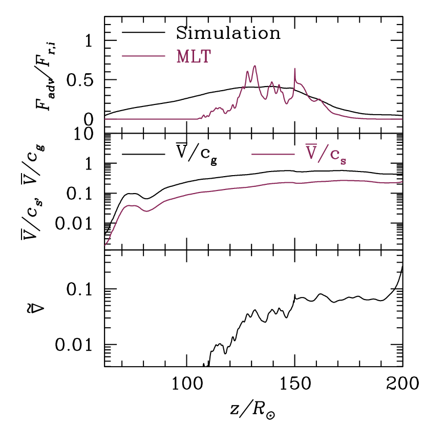
Figure 6.— Top: horizontally and time averaged advection flux $F_{\rm adv}=v_{z}E_{r}$ (black line) for the run StarDeep. The red line is the convection flux calculated according to equation (17) based on the horizontally and time averaged vertical profiles of temperature and pressure in the same run with mixing length parameter $\alpha=0.55$. Middle: horizontally and time averaged turbulent velocity $\bar{V}$ (equation 12), scaled with radiation sound speed $c_{s}$ (red line) and isothermal sound speed $c_{g}$ (black line) at each height. Bottom: vertical profile of $\tilde{\nabla}\equiv(\nabla-\nabla_{\text{ad}})/\nabla_{\text{ad}}$ for the run StarDeep. The actual gradient $\nabla\equiv d\ln T/d\ln(P+P_{r})$ is calculated based on the horizontally and time averaged temperature and pressure profiles. The adiabatic gradient is close to $0.25$ for the radiation dominated envelope. The fact that $\tilde{\nabla}\ll 1$ implies that the convection is almost adiabatic.

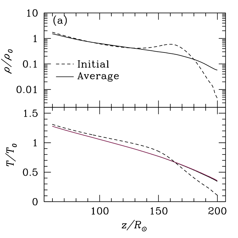
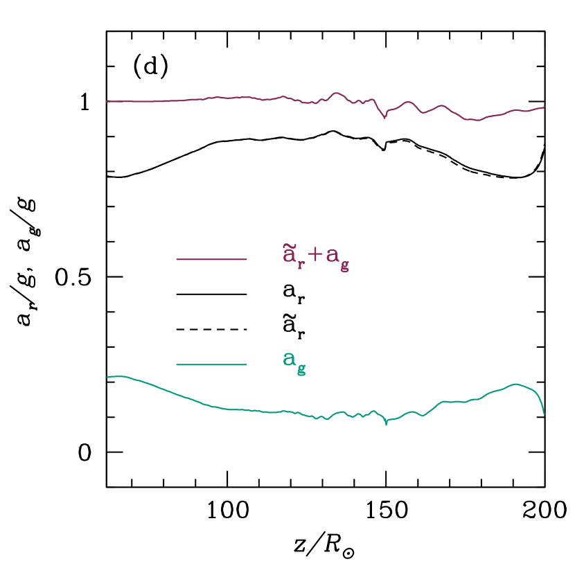
Figure 7.— Horizontally and time averaged vertical profiles of various quantities for the run StarDeep. Panel (a): density (solid line at top), gas temperature (solid black line at bottom) and radiation temperature (solid red line at bottom). The gas and radiation temperature profiles overlap as they are strongly thermally coupled. Panel (b): gas entropy $S_{g}$ (solid black line at top) and radiation entropy $S_{r}$ (solid black line at bottom). These entropies are calculated according to equation (9), and both are in units of $\mathrm{k_{B}}/\mu$. Panel (c): total opacity $\kappa_{t}$ in unit of $1/(\rho_{0}H_{0})$ (the solid line). The dashed black lines in these three panels are the initial conditions. Panel (d): volume averaged (solid black line) and density weighted (dashed black line) radiation accelerations ($a_{r}$, $\tilde{a}_{r}$) as well as the acceleration due to the gas pressure gradient ($a_{g}$, green line). The red line is the sum of $\tilde{a}_{r}$ and $a_{g}$. In this run with $\tau_{0}\gg\tau_{c}$, the density inversion in the initial condition is gone.

In the 3D radiation hydrodynamic simulations, energy can be transported vertically by either photon diffusion or turbulent transport. We quantify the turbulent transport using the advection flux $F_{\rm adv}$, which is

$$F_{\rm adv}=v_{z}E_{r}.$$ (11)

In principle, photon advection can be due to either a mean flow (e.g., an outflow) or turbulence. In our simulations, the latter dominates.

The solid line in the top panel of Figure 6 shows the time averaged advective radiation flux $F_{\rm adv}$ as a function of height where the time average is done between $31t_{0}$ and $107t_{0}$. Most of the flux at $z<100R_{\odot}$ is carried by radiative diffusion. In the turbulent region between $z=110R_{\odot}$ and $160R_{\odot}$, however, the averaged advection flux is more than $40\%$ of $F_{r,i}$. We compare this to MLT in the next section.

The turbulent velocity in the envelope can be quantified as

$$\overline{V}=\sqrt{\frac{\int\rho\bm{v}\cdot\bm{v}dV}{\int\rho dV}}.$$ (12)

The middle panel of Figure 6 shows the time averaged vertical profile of this turbulent velocity relative to both the isothermal sound speed $c_{g}=\sqrt{P/\rho}$ and the radiation sound speed $c_{s}=\sqrt{E_{r}/(3\rho)}$ . The averaged turbulent velocity is only $6-20\%$ of the radiation sound speed in the turbulent region. Even compared with the isothermal sound speed alone, $\overline{V}/c_{g}$ is smaller than $0.4$. This implies that in the efficient convection regime, the turbulent kinetic energy density is much smaller than the thermal energy density ($\lesssim 2\%$), as expected.

Figure 7 shows the quasi-steady envelope structure compared with the hydrostatic initial condition. Note that the density and temperature are relatively unaffected near the bottom of the box indicating that we have placed the bottom boundary deep enough. In the final quasi-steady envelope, the iron opacity peak moves slightly deeper relative to the initial condition, but the density inversion present in the initial condition is gone. This is consistent with the 1D MESA models which also find that for the conditions in StarDeep mixing length theory predicts that convection is efficient and is able to remove the density inversion. Note that the location where the advection flux is largest ($z\approx 120R_{\odot}$ in Fig. 6) corresponds to the location of the iron opacity peak in the final state. This is also where the radiation entropy $S_{r}$ decreases with height, consistent with convection continuing to drive the turbulent motions and energy transport. As expected, the radiation entropy profile is also flatter in the turbulent state after the density inversion is removed.

Because part of the energy flux in the turbulent state is carried by advection, the averaged diffusive flux also drops below the initial value $F_{r,i}$. The significant contribution of the advection flux reduces the radiation acceleration so that it is smaller than the gravitational acceleration. The accelerations due to gas $a_{g}$ and radiation $a_{r}$ can be calculated as

$$a_{g}=-\frac{1}{\rho}\frac{\partial P}{\partial z},$$

$$a_{r}=\frac{\kappa_{t}}{c}F_{r,0z}.$$ (13)

Notice that only the diffusive radiation flux $F_{r,0z}$ contributes to the radiation acceleration, which is the radiation pressure gradient in the optically thick regime. The last panel of Figure 7 shows that gravity is roughly balanced by the sum of radiation and gas pressure gradients, with $a_{r}$ being at most $90\%$ of $g$. The fact that $a_{r}\lesssim g$ is consistent with the absence of a density inversion in the turbulent state.

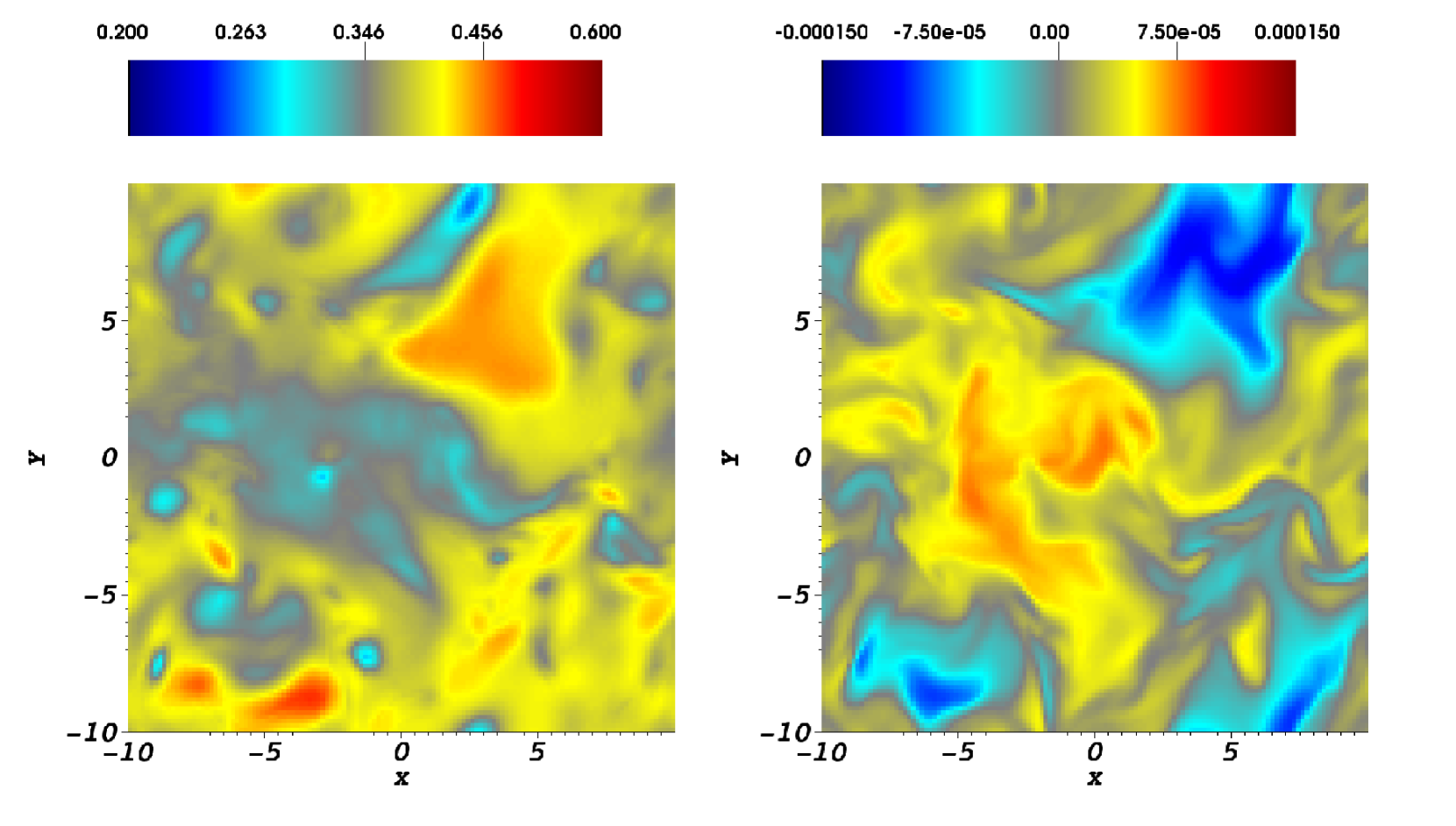
Figure 8.— Horizontal slices of density $\rho$ (left) and vertical component of the radiation flux $F_{r,z}$ (right) at $z=140R_{\odot}$ for the run StarDeep at time $97.8t_{0}$. The box size is in units of $R_{\odot}$ while units for $\rho$ and $F_{r,z}$ are $\rho_{0}$ and $ca_{r}T_{0}^{4}$ respectively. Notice the strong anti-correlation between $\rho$ and $F_{r,z}$ caused by buoyancy.

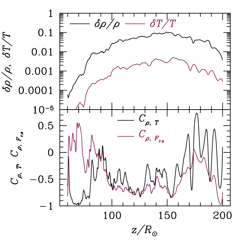
Figure 9.— Top: vertical profiles of standard deviations of density $\rho$ and temperature $T$ at time $97.8t_{0}$ for the run StarDeep. The standard deviations are scaled with the mean density and temperature at each height. Bottom: Vertical profiles of cross correlation coefficients between $\rho$, $T$ and $\rho$, $F_{r,z}$ at the same time. The anti-correlation between $\rho$ and $F_{r,z}$ in this run is due to the buoyancy instead of the “porosity” effect, as $F_{r,z}$ is dominated by the advection flux $v_{z}E_{r}$.

4.1.3 Time Averaged Horizontal Structures

Figure 8 shows horizontal slices of density $\rho$ and the vertical component of Eulerian radiation flux $F_{r,z}$ at $z=140R_{\odot}$ and time $97.8t_{0}$ for the run StarDeep. There is a clear anti-correlation between fluctuations of $\rho$ and $F_{r,z}$. When $\rho$ is larger (smaller) than the horizontally averaged density, $F_{r,z}$ is negative (positive). This is a natural outcome of convection, where the Eulerian radiation flux $F_{r,z}$ is dominated by the advection part $v_{z}E_{r}$ at each location in the regime $\tau_{0}\gg\tau_{c}$. Figure 8 thus shows that low density regions buoyantly rise while high density fluid elements fall.

To quantify the level of density and temperature fluctuations, the top panel of Figure 9 shows the vertical profiles of standard deviations of $\rho$ and $T$ scaled with the horizontally averaged mean values at each height at time $97.8t_{0}$. The scaled standard deviations peak at $150R_{\odot}$, where the iron opacity peak is located at this time. Beyond the convective region, fluctuations drop with height. The scaled density standard deviation is always smaller than $10\%$ in this case. Temperature fluctuations ($\lesssim 0.4\%$) are much smaller. Because radiation pressure $P_{r}\propto T^{4}$, the pressure fluctuations are only $\lesssim 1.6\%$.

The cross correlation between two quantities $a$ and $b$ can be quantified by the correlation coefficient $C_{a,b}$, normalized by their standard deviations $\sigma_{a},\sigma_{b}$. The bottom panel of Figure 9 shows the correlation coefficients between $\rho,T$ and $\rho,F_{r,z}$. Consistent with the slice shown in Figure 8, there is an anti-correlation between $\rho$ and $F_{r,z}$ in the convective region due to buoyancy. Temperature fluctuations also anti-correlate with density fluctuations, which means an anti-correlation between density $\rho$ and radiation pressure $P_{r}$. In this very optically thick regime $\tau_{0}\gg\tau_{c}$, density fluctuations do not reduce the effective radiation acceleration, which can be confirmed by comparing the volume averaged $a_{r}$ (equation 13), and the density weighted radiation acceleration

$$\tilde{a}_{r}=\frac{\langle\rho\kappa_{t}F_{r,0z}\rangle}{c\langle\rho\rangle}.$$ (14)

Here the average $\langle\cdot\rangle$ is done horizontally at each height. Panel (d) of Figure 7 shows vertical profiles of the time averaged radiation accelerations calculated in these two different ways. They are almost identical. This explictly demonstrates that there is no reduction of the radiation acceleration due to density fluctuations in this regime.

The typical size of the turbulent structures can be estimated by calculating the normalized cross correlation $C_{\rho,\tilde{\rho}}$ between $\rho(x,y)$ and $\rho(x+l_{\rho},y+l_{\rho})$, where $\rho(x+l_{\rho},y+l_{\rho})$ is the density shifted horizontally with distance $l_{\rho}$. The correlation length $l_{\rho}$ can be defined to to be the shifted distance when $C_{\rho,\tilde{\rho}}$ drops to zero. For the run StarDeep, $l_{\rho}$ is typically $\sim 0.3-0.4H_{0}$, with corresponding optical depth at the iron opacity peak comparable to $c/c_{s,0}$ given in Table 1.

4.1.4 Comparison with Mixing Length Theory

In the radiation dominated regime, the radiation advection flux $F_{\rm adv}$ from the simulations can be directly compared with the convection flux from MLT. We define the ratio of gas pressure to total pressure ($\beta$), the first ($\Gamma_{1}$) and second ($\Gamma_{2}$) adiabatic indices, and specific heat at constant pressure ($c_{p}$) for a mixture of gas and radiation (Chandrasekhar, 1967), and the logarithmic derivative of density with respect to temperature at constant total pressure to be

$$\beta \equiv \frac{P}{P+P_{r}},$$

$$\Gamma_{1} \equiv \beta+\frac{(4-3\beta)^{2}(\gamma-1)}{\beta+12(\gamma-1)(1-\beta)},$$

$$\Gamma_{2} = \frac{(4-3\beta)\Gamma_{1}}{3(1-\beta)\Gamma_{1}+\beta}$$

$$c_{p} = \frac{1}{\gamma-1}\frac{\Gamma_{1}}{\beta^{2}}\left[\beta+12(\gamma-1)(1-\beta)\right],$$

$$Q \equiv -\left.\frac{d\ln\rho}{d\ln T}\right|_{P+P_{r}}=\frac{4-3\beta}{\beta},$$ (15)

where $P_{r}$ is the $zz$ component of the radiation pressure tensor ${\sf P_{r}}$. The adiabatic temperature gradient with respect to total pressure can be calculated as

$$\nabla_{\text{ad}}\equiv\left.\frac{d\ln T}{d\ln(P+P_{r})}\right|_{\text{ad}} = \frac{\Gamma_{2}-1}{\Gamma_{2}}.$$ (16)

The actual gradient $\nabla\equiv d\ln T/d(\ln(P+P_{r}))$ can be calculated based on the mean density and temperature profiles shown in Figure 7. If we assume that the mixing length is related to the pressure scale height via the mixing parameter $\alpha$, then the convective flux based on non-adiabatic mixing length theory including the effects of radiative cooling is (Henyey et al., 1965)

$$F_{\text{conv}}=\frac{Q^{1/2}c_{p}}{4\sqrt{2}}\frac{\mathrm{k_{B}}\rho T}{\mu}\left(\frac{P+P_{r}}{\rho}\right)^{1/2}\alpha^{2}\left(\nabla-\nabla^{\prime}\right)^{3/2},$$

(17)

assuming that the radiation entropy $S_{r}$ decreases with height. Here the gradient $\nabla^{\prime}$ is calculated based on equations (32) and (42) in Henyey et al. (1965) given the mean vertical profiles of the envelope. In the adiabatic limit, $\nabla^{\prime}$ is reduced to $\nabla_{\text{ad}}$. Then equation 17 is the same as the formula given by the adiabatic mixing length theory (Cox, 1968).

The convective flux calculated in this way with $\alpha=0.55$ is shown as the red line in the top panel of Figure 6, which agrees with the time averaged advection flux in the simulation. Note that the value of $\alpha$ required to explain the flux in the simulations is also quite close to the ratio between the density correlation length and pressure scale height $H_{0}$ (see Section 4.1.3), which is the definition of $\alpha$ in mixing length theory. Finally, Figure 6 shows that the difference between the actual gradient and the adiabatic gradient $\tilde{\nabla}\equiv(\nabla-\nabla_{\text{ad}})/\nabla_{\text{ad}}$ is quite small, consistent with the expectations of efficient convection.

Taken together, these comparisons demonstrate that the statistical properties of the turbulent energy transport in our radiation hydrodynamic simulation with $\tau_{0}\gg\tau_{c}$ are reasonably consistent with the expectations of mixing length theory, although the value of $\alpha$ is somewhat smaller than traditionally assumed in models of massive stars (typical values $\alpha=1.0...1.5$, see e.g. Yusof et al., 2013; Köhler et al., 2015). This is the first numerical confirmation of the adequacy of MLT in a radiation dominated regime.

4.2. The run StarMid when $\tau_{0}\gtrsim\tau_{c}$

In this regime, rapid radiative diffusion starts to have a non-negligible impact on the properties of convection in the radiation dominated stellar envelope (the typical thermal time scale near the iron opacity peak is $\sim 5$ dynamical times). Compared with the previous run, we shall see the effects of the reduced optical depth. Note that unlike StarDeep, the photosphere is captured within the domain of this simulation.

4.2.1 Simulation History

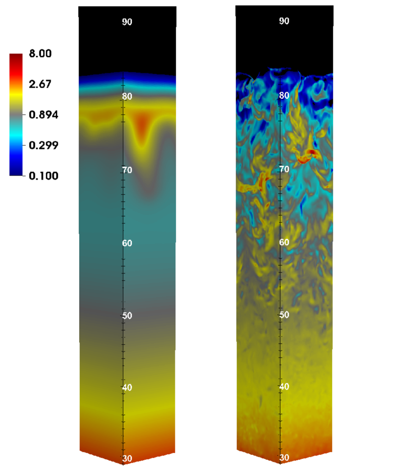
Figure 10.— Snapshots of density for the run StarMid at time $9.4t_{0}$ (left) and $18.8t_{0}$ (right). The box size is in units of $R_{\odot}$ while the density unit $\rho_{0}$ is given in Table 1. The horizontal box sizes are $L_{x}=L_{y}=10R_{\odot}$.

Figure 11.— History of the volume averaged vertical velocities $V_{z,E_{r}}$ and $V_{z,\rho}$ for the run StarMid.

The initial condition for StarMid has the iron opacity peak and density inversion at $78R_{\odot}$. The density inversion region is, however, convectively unstable and starts to mix at time $9.4t_{0}$ as shown in the left panel of Figure 10. At time $18.8t_{0}$, the whole envelope is turbulent (right panel of Fig. 10). This temporal evolution is very similar to the run StarDeep, but the properties of the turbulence are different as we now describe.

Figure 11 shows the radiation energy density and density weighted vertical velocities ($V_{z,E_{r}},V_{z,\rho}$) as a function of time. After the initial density inversion is broken around $10t_{0}$, $2.4\%$ of the mass is lost through the open top boundary. The averaged vertical velocity also reaches the peak at the same time. The whole envelope oscillates with a period of $4t_{0}$. The vertical velocities can reach $10\%$ of the typical radiation sound speed, which is much larger than the oscillation amplitude in StarDeep (Figure 5). When the envelope expands, it is accelerated by the radiation without the density inversion. But because of the sensitive dependence of the iron opacity on temperature and the temperature decrease with height, the radiation acceleration becomes smaller than $g$ at some height and the acceleration stops. The whole envelope starts to fall back when the vertical velocity reverses.

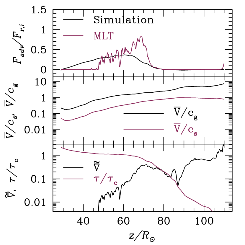
Figure 12.— Top: time and horizontally averaged vertical profiles of advection flux (black line) and convection flux predicted by mixing length theory (red line). Middle: the averaged turbulent velocity $\overline{V}$ scaled with the radiation sound speed $c_{s}$ (red line) and isothermal sound speed (black line). Bottom: vertical profile of the superadiabatic parameter $\tilde{\nabla}$ (black line) and the ratio between the local optical depth per pressure scale height $\tau$ and the critical value $\tau_{c}$ (red line). These profiles are for the run StarMid and the time average is done between $17.6t_{0}$ and $29.2t_{0}$.

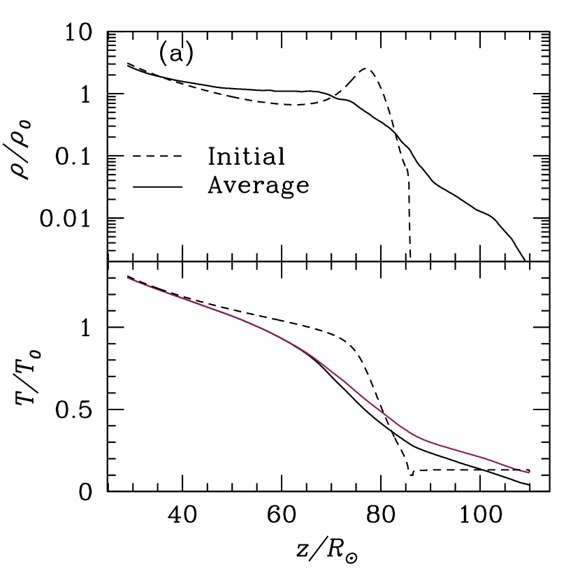
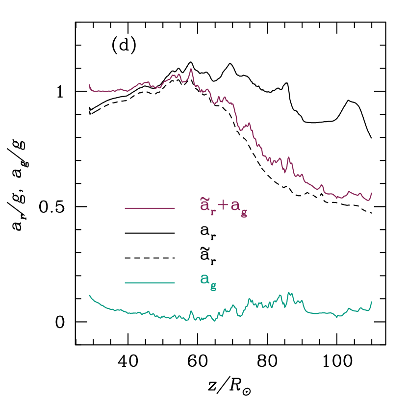
Figure 13.— The time and horizontally averaged vertical profiles of density (top panel of a), temperature (bottom panel of a, solid black line for gas temperature and red line for radiation temperature), entropy (panel b), opacity (panel c) as well as accelerations (panel d) for the run StarMid. As in Figure 7, the dashed lines in panels (a), (b), (c) are initial conditions while other lines are time averaged profiles. The initial condition above $85R_{\odot}$ is the region above the photosphere where we set it to be isothermal.

4.2.2 Time Averaged Vertical Structure and Turbulent Properties

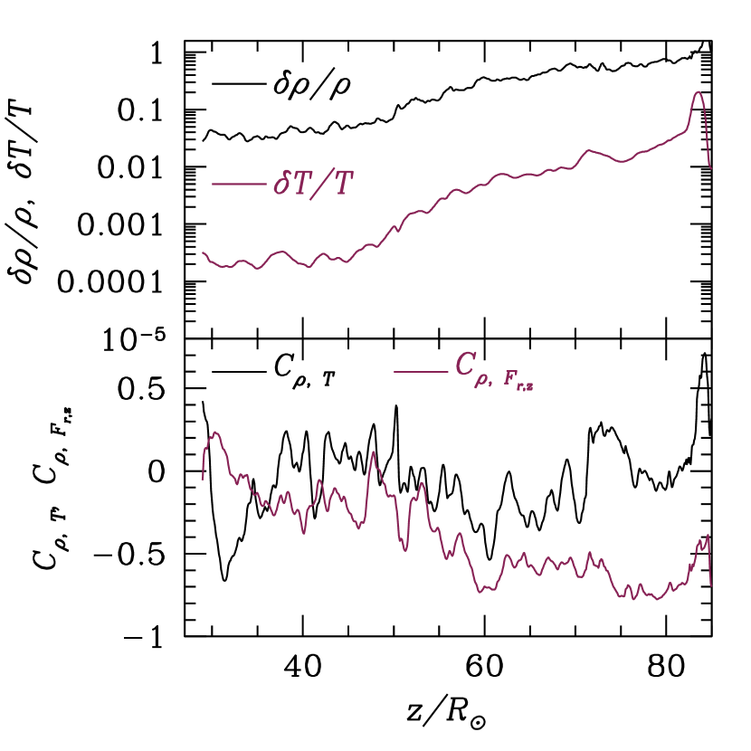
Figure 14.— Top: vertical profiles of density and temperature standard deviations scaled with the horizontally averaged mean values. Bottom: vertical profiles of cross correlation coefficients between $\rho,T$ and $\rho,F_{r,z}$. These profiles are for the run StarMid at time $18.8t_{0}$.

Figure 12 (solid line) shows that there is significant turbulent transport of energy below $65R_{\odot}$, but the turbulent transport falls off rapidly at larger heights. At about the same location $65R_{\odot}$, the averaged turbulent velocity $\overline{V}$ reaches the isothermal sound speed (middle panel of Fig. 12), but is still smaller than the radiation sound speed.

Figure 13 shows the time and horizontally averaged vertical profiles of density, temperature, opacity, entropy and accelerations for this run. The iron opacity peak moves inward somewhat in radius, but the density inversion in the initial condition is largely gone, replaced with an extended region below $65R_{\odot}$ over which the density changes very slowly with height. Gas and radiation are thermally coupled in this region. However, above $65R_{\odot}$, the density drops quickly with height and the gas temperature starts to deviate from the radiation temperature. Here the local optical depth per pressure scale height $\tau$ becomes smaller than the critical value $\tau_{c}$ and the photon diffusion time becomes smaller than the local dynamic time. This transition to $\tau\lesssim\tau_{c}$ is why the advection flux drops significantly in this region (Fig. 12).

The top panel of Figure 12 shows the convective flux calculated based on the time averaged vertical profiles and mixing length theory (eq. 17) with $\alpha=0.45$, which is again close to the ratio between the correlation length $l_{\rho}$ and scale height $H_{0}$. Below $60R_{\odot}$ where $\tau>\tau_{c}$, the time averaged advection flux is comparable to the mixing length theory convection flux, which is consistent with Figure 6 for the run StarDeep. However, above $65R_{\odot}$ the advection flux drops significantly in the simulations, but equation (17) still predicts a very large convection flux because of the decreasing radiation entropy (see panel b of Fig 13). This demonstrates that for $\tau\lesssim\tau_{c}$, convection becomes inefficient and equation (17) significantly overestimates the amount of advection flux with a constant $\alpha$.

The vertical profile of $\tau/\tau_{c}$, where $\tau=\rho\kappa_{t}H_{0}$ is the local optical depth per pressure scale height, shown in the bottom panel of Figure 12 confirms that the transition to inefficient convection happens when $\tau/\tau_{c}<1$. It also happens roughly when the turbulent velocity $\overline{V}$ becomes larger than the isothermal sound speed (the middle panel of Figure 12), and the superadiabatic parameter $\tilde{\nabla}$ increases significantly to $\sim 0.4$ (bottom panel of Figure 12). Notice that throughout the whole envelope, $\tilde{\nabla}$ is comparable to $\overline{V}/c_{s}$ as in Figure 6 for the case StarDeep.

Panel (d) of Figure 13 shows that the volume averaged radiation acceleration $a_{r}$ is larger than the gravitational acceleration between $50R_{\odot}$ and $80R_{\odot}$, which is also the region where radiation entropy decreases with height. It is thus perhaps surprising that when convection becomes inefficient above $65R_{\odot}$ and there is little turbulent transport of energy, the envelope does not develop a density inversion again. This is because the density weighted radiation acceleration $\tilde{a}_{r}$ (eq . 14, shown as the dashed black line in panel (d) of Figure 13) is significantly smaller than the volume averaged radiation acceleration $a_{r}$ above $65R_{\odot}$. The sum $\tilde{a}_{r}+a_{g}$ is comparable to $g$ at the iron opacity peak around $60R_{\odot}$. Beyond $65R_{\odot}$, it drops below $g$ significantly.

Figure 14 clarifies the origin of the reduced density weighted radiation acceleration. In particular, it shows that density fluctuations reduce the effective radiation acceleration above $65R_{\odot}$ because there is an anti-correlation between fluctuations of density and radiation flux. The correlation coefficient $C_{\rho,F_{r,z}}$ in Figure 14 shows this explicitly and is always negative. However, the nature of the anti-correlations changes at different heights. Below $65R_{\odot}$, when $\tau>\tau_{c}$, the situation is similar to the run StarDeep, in that buoyancy causes the anti-correlation between $\rho$ and $F_{r,z}$, as $F_{r,z}$ is dominated by the advection flux. Above $65R_{\odot}$, however, when $\tau\lesssim\tau_{c}$, the situation changes. Convection becomes inefficient and $F_{r,z}$ is dominated by the diffusive flux (the advection flux drops as shown in Figure 12). The anti-correlation between $\rho$ and $F_{r,z}$ above $65R_{\odot}$ is thus not caused by buoyancy. Instead, it is because the “porosity” of the envelope created by the traveling strong shocks allows radiation to propagate through low density regions (Shaviv, 1998). This reduces the effective radiation acceleration significantly (see panel (d) of Figure 13). Note also that in StarMid, the standard deviations of density and temperature (scaled with the horizontally averaged quantities) are significantly larger than the corresponding values in the run StarDeep (Figure 9).

4.3. The run StarTop when $\tau_{0}\ll\tau_{c}$

This is the regime when gas and photons are loosely coupled through the whole iron opacity peak region. Convection will be inefficient as in the top region of StarMid. The photosphere is now closer to the region with the iron opacity peak and accurate radiation transfer is critical. For this run, we use a density floor of $10^{-10}\rho_{0}$ to avoid numerical difficulties.

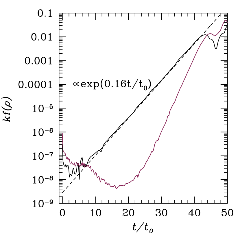
Figure 15.— Time evolution of the density power spectrum $kf(\rho)$ for the run StarTop at height $z=13.7R_{\odot}$ during the first $50t_{0}$. The solid black and red lines are for the modes with wavelength $H_{0}$ and $0.26H_{0}$ respectively. The long wavelength mode has an e-folding time $6.25t_{0}$ as indicated by the dashed black line.

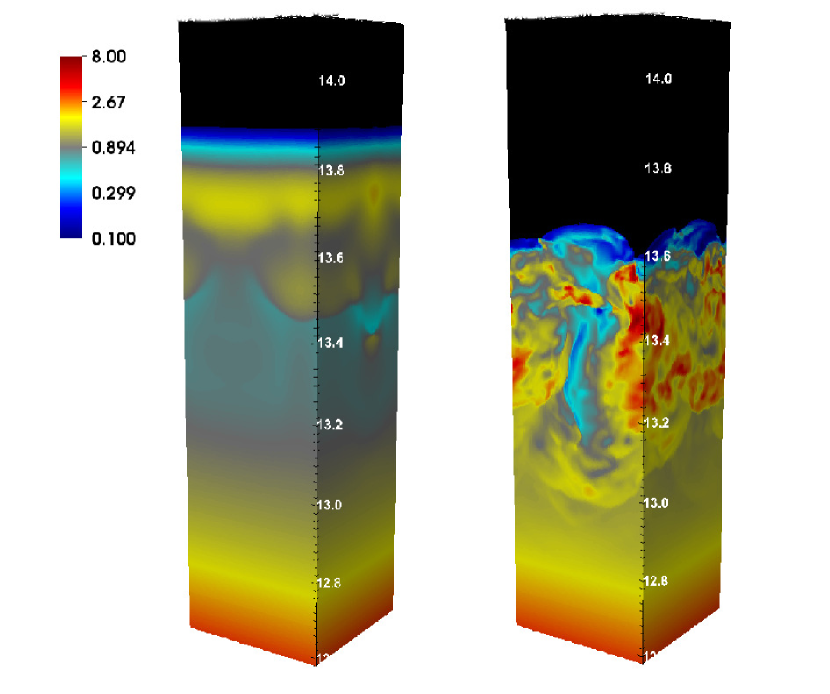
Figure 16.— Snapshots of density for the run StarTop at time $49.1t_{0}$ (left) and $138.9t_{0}$ (right).

Figure 17.— History of the volume averaged vertical velocity $V_{z,E_{r}}$ (solid line at bottom) and $V_{z,\rho}$ (dashed line at bottom) for the run StarTop. The volume average is done for the whole simulation box.

4.3.1 Simulation History

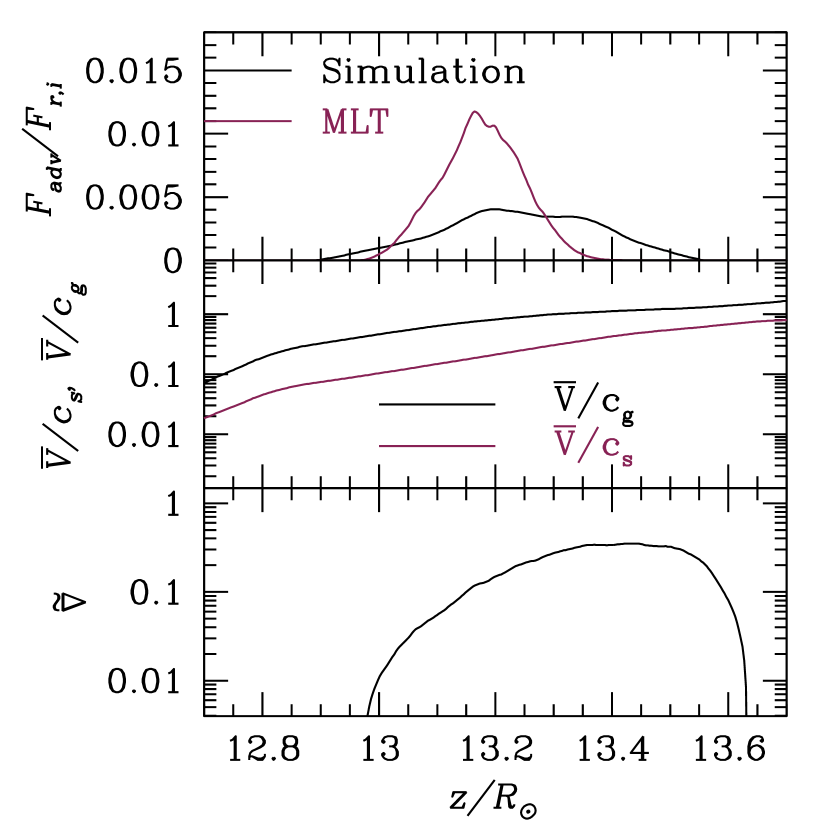
Figure 18.— Top: time and horizontally averaged vertical profiles of advection flux (black line), and convection flux according to the non-adiabatic MLT with $\alpha=0.4$ (equation 17) as given by Henyey et al. (1965) (red line). Middle: the averaged turbulent velocity $\overline{V}$ scaled with the radiation sound speed $c_{s}$ (red line) and isothermal sound speed (black line). Bottom: vertical profile of superadiabatic parameter $\tilde{\nabla}$. The time average is done between $55.6t_{0}$ and $171.0t_{0}$. These profiles are for the run StarTop.

The iron opacity peak and density inversion are located at $13.7R_{\odot}$ initially. This is again convectively unstable and the initial structure is completely destroyed by $50t_{0}$. Just as we found in the simulation StarDeep, this time scale is significantly longer than the buoyancy time scale $1/|N_{r}|$, which is $\approx t_{0}$ at the iron opacity peak. We therefore again explored the linear growth phase for this run by calculating the density power spectrum at the location of the initial density inversion. The time evolutions of the power $kf(\rho)$ in two modes with horizontal wavelengths $H_{0}$ and $0.26H_{0}$ are shown in Figure 15. As in StarDeep (Fig. 4), the long wavelength mode grows exponentially from close to the beginning, with an e-folding time of $6.25t_{0}$. However, in contrast to the StarDeep case, the short wavelength mode is damped initially and only starts to grow quickly after $20t_{0}$ when the e-folding time is $3.33t_{0}$. This later rapid growth is almost certainly due to a nonlinear cascade.

We have examined the behavior of other horizontal wavelengths as well, and found that all the modes with horizontal wavelengths larger than $\approx 0.4H_{0}$ have similar growth rates after $12t_{0}$, while the modes with horizontal wavelengths smaller than $\approx 0.3H_{0}$ are damped until the nonlinear cascade sets in. Based on the analysis of Blaes & Socrates (2003), we estimate that modes with wavelengths less than about $2.5H_{0}$ are in the regime where radiative diffusion reduces the growth rate of the convective instability. This is larger than the size of the box, so that all convective modes in the simulation are heavily modified by radiative diffusion (consistent with the fact that $\tau_{0}\lesssim\tau_{c}$). From equation (59) of Blaes & Socrates (2003), we find that the long wavelength mode in Figure 15 should have a growth rate of $\simeq 0.17/t_{0}$, assuming a vertical wavelength that is comparable to the horizontal wavelength (which is also comparable to the vertical width of the density inversion). This agrees very well with the measured growth rate. However, shorter wavelength modes should have smaller growth rates $\propto k^{-2}$, in contrast to the behavior measured in the simulations. It is not clear what is causing this discrepancy, although we suspect that the damping of modes with wavelength $\lesssim 0.3H_{0}$ is due to the numerical damping rate being larger than the very small growth rate for these modes. Interestingly, traveling acoustic waves should also be unstable according to equation (62) of Blaes & Socrates (2003), with comparable growth rates to the buoyancy instability (such waves should not be unstable in the StarDeep simulation). Vertically propagating acoustic waves (with infinite horizontal wavelength) should grow fastest, but these would not necessarily show up as growing perturbations at a fixed height. We have not further investigated this possibility, as it is clear that the unstable buoyancy modes dominate the evolution observed in the simulation.

Figure 16 shows snapshots of the density structure of the envelope at time $49.1t_{0}$ and $138.9t_{0}$ while the histories of the vertical velocities $V_{z,E_{r}},V_{z,\rho}$ are shown in Figure 17. The whole envelope becomes turbulent after the initial density inversion is destroyed around $50t_{0}$. Unlike the simulations StarDeep and StarMid, the turbulent envelope is not a relatively quiescent convective structure, but instead shows violent, irregular, large amplitude oscillations. The oscillation period varies from $\sim 5$ to $10t_{0}$. The amplitude of $V_{z,E_{r}}$ is $0.05c_{s,0}$, which is already $\approx 18\%$ of the isothermal sound speed. At time $138.9t_{0}$ when $V_{z,E_{r}}$ reaches a minimum, the right panel of Figure 16 shows that there is even a low density hole extending over one pressure scale height $H_{0}$. The mass loss through the open top boundary is negligible for this run.

According to equation (3), the typical thermal time scale is $t_{c}\sim 0.09t_{0}$ for this run. However, for this $\tau_{0}\ll\tau_{c}$ regime, $t_{c}$ is no longer the most relevant time scale for some of the dynamics. Instead, the radiation flux behaves like a roughly constant force reducing the effective gravity (Jiang et al., 2013a). The more relevant time scale is the effective dynamic time scale

$$\tilde{t}_{0}\equiv\frac{c_{g,0}}{|\tilde{g}|},$$ (18)

where $c_{g,0}$ is the isothermal sound speed and $\tilde{g}\equiv g-\tilde{a}_{r}$ is the effective acceleration due to gravity and the radiation force. For an effective acceleration $\tilde{g}=-0.06g$ according to the $\tilde{a}_{r}$ shown in panel (d) of Figure 19 (discussed below), the effective dynamic time scale is $\tilde{t}_{g}=4.6t_{0}$, which is consistent with the oscillation period of the envelope in Figure 17. Note that the effective scale height is then $\tilde{H}_{0}\equiv c_{g,0}^{2}/|\tilde{g}|=1.26H_{0}$, which happens to be similar to $H_{0}$.

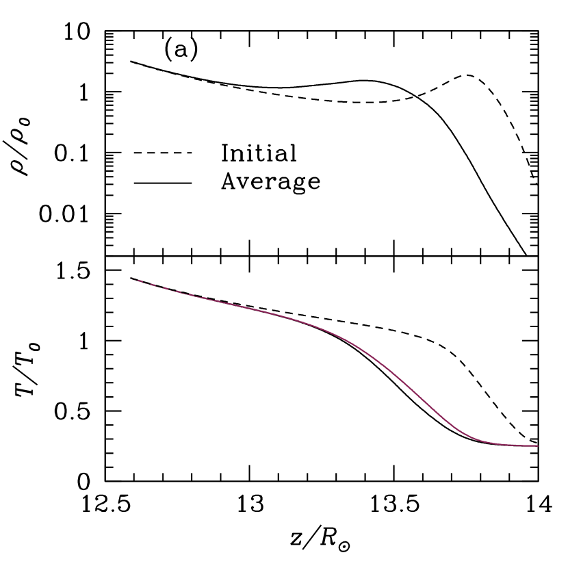
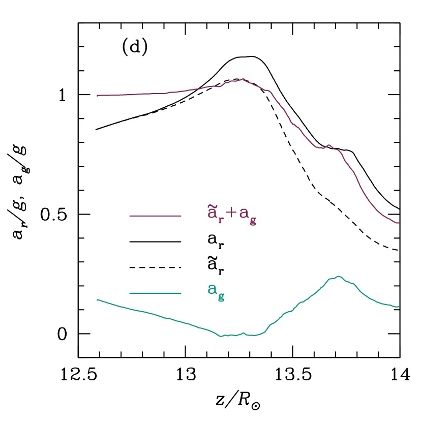
Figure 19.— The time and horizontally averaged vertical profiles of density (top panel of a), temperature (bottom panel of a, black and red lines for gas and radiation temperature), entropy (panel b), opacity (panel c) as well as accelerations (panel d) for the run StarTop. The dashed lines in (a), (b) and (c) are initial conditions while other lines are time averaged profiles between $55.6t_{0}$ and $171.0t_{0}$.

4.3.2 Time Averaged Vertical Structures

Figures 18 and 19 show vertical profiles of various time and horizontally averaged quantities in the nonlinear state after $55.6t_{0}$. Unlike the previous two runs StarDeep and StarMid, the averaged advection flux is less than $0.5\%$ of $F_{r,i}$ in the whole envelope as shown in the top panel of Figure 18. This is because $\tau_{0}\ll\tau_{c}$ everywhere and gas is not able to trap photons. The averaged radiation flux $F_{r,0z}$ is almost a constant vertically except very near the top of the domain; the radiation flux is nearly constant in time as well, with $\lesssim 8\%$ variation during the whole simulation.

Because the radiation flux dominates over the advection flux, the full super-Eddington flux contributes to the radiation acceleration of the gas. However, because of the large density fluctuations, most photons go through regions that have below average density. This reduces the density weighted radiation acceleration $\tilde{a}_{r}$ (eq. 14), as shown in panel (d) of Figure 19. However, unlike the assumptions made in previous models (Shaviv, 1998), the “porosity” of the envelope due to convection cannot reduce the effective radiation acceleration to a value below $g$. At $z\approx 13.3R_{\odot}$ where the iron opacity peak is located now, $\tilde{a}_{r}$ is still about $6\%$ larger than $g$, while $a_{r}$ is about $10\%$ larger than $g$. This is why the average density profile still shows a mild inversion near the iron opacity peak, as shown in panel (a) of Figure 19. We stress that although the density inversion remains, the resulting structure is nonetheless very different from the hydrostatic density inversion in the initial condition. The high density region near the iron opacity peak is continuously reformed and then mixed, triggering violent oscillations, shocks, and large density fluctuations in the stellar envelope. Physically, in the regime $\tau_{0}\ll\tau_{c}$, photon diffusion is so rapid that radiation pressure does not respond to the density and velocity fluctuations. As the turbulent velocity becomes larger than the isothermal sound speed, shocks are formed in the envelope (Figure 16), which causes the large density fluctuations. This phenomenon is also observed in radiation magneto-hydrodynamic simulations of black hole accretion disks (Turner et al., 2003; Jiang et al., 2013c).

Figure 19 shows that the radiation and gas entropies $S_{r}$ and $S_{g}$ decrease rapidly with height around the iron opacity peak. If we still adopt $l_{\rho}/H_{0}\approx 0.4$ for the mixing length parameter $\alpha$, equation (17) over-predicts the flux relative to the simulations by a factor of more than $\sim 3$, and the location of the peak in the predicted flux also offsets from the peak of time averaged advection flux given by the simulations, highlighting that existing models of inefficient convection in the radiation pressure dominated regime are not accurate compared to our simulation results. The failure of convection to carry a significant energy flux is intimately connected with the turbulent velocities becoming supersonic, at least relative to the gas (isothermal) sound speed. This is expected on theoretical grounds (§2) and is also consistent with the simulation results, as shown in the middle panel of Figure 18. The superadiabatic parameter $\tilde{\nabla}$ is also comparable to $\tilde{V}/c_{s}$ and similar to the top region in StarMid (Figure 12).

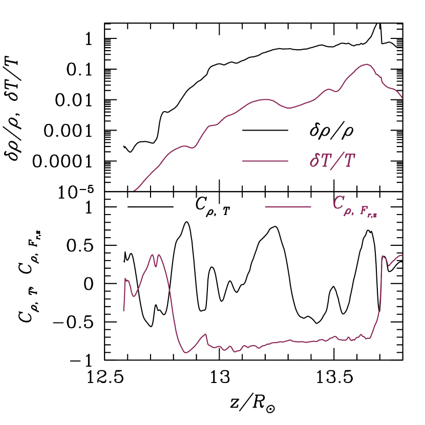
Figure 20.— Top: vertical profiles of density and temperature standard deviations scaled with the horizontally averaged mean values. Bottom: vertical profiles of cross correlation coefficients between $\rho,T$ and $\rho,F_{r,z}$. These profiles are for the run StarTop at time $138.9t_{0}$.

4.3.3 Properties of the Turbulent Structures

Figure 20 quantifies the large density fluctuations and strong anti-correlation between density and radiation flux in simulation StarTop. The correlation coefficient $C_{\rho,F_{r,z}}$ is almost $-1$ in the turbulent region between $12.8R_{\odot}$ and $13.6R_{\odot}$, while $C_{\rho,T}$ only fluctuates around $0$. This demonstrates that unlike for StarDeep, the anti-correlation between density and radiation flux is not due to buoyancy in the radiation pressure dominated regime but is instead due to the photons preferentially diffusing through low density channels. The scaled standard deviations $\delta\rho/\rho$ and $\delta T/T$ are also much larger than the corresponding values in StarDeep and StarMid, which is consistent with the images in Figure 16.

The typical size of the turbulent structures can also be quantified by the correlation length $l_{\rho}$, which varies between $0.4H_{0}$ and $0.5H_{0}$. This is likely set primarily by geometry as in standard mixing length arguments. In particular, the optical depth across the correlation length $\tau_{l}$ is much smaller than $\tau_{c}$, which means that photon diffusion is very rapid for all of the turbulent fluctuations and cannot be important for setting a characteristic scale. The correlation length $l_{\rho}$ is also much smaller than the characteristic turnover wavelength of acoustic waves driven unstable by the dependence of opacity on density (Blaes & Socrates, 2003). Once again, it is simply the fact that the convective turbulence is supersonic with respect to the isothermal sound speed in the gas, and that radiation pressure cannot respond due to the rapid diffusion, that is producing these nonlinear structures.

5. Discussions and Conclusions

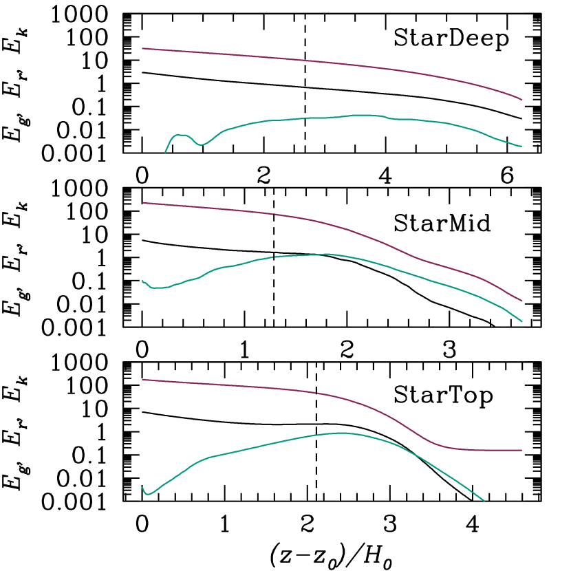
Figure 21.— Time and horizontally averaged vertical profiles of radiation energy density ($E_{r}$, red lines), gas internal energy density ($E_{g}$, solid black lines) and kinetic energy density ($E_{k}$, green lines). From top to bottom, they are for StarDeep, StarMid and StarTop respectively. The black dashed vertical lines in each panel indicate the time averaged location of the iron opacity peak. The horizontal axis is the distance from the bottom boundary $z_{0}$ in units of the scale height $H_{0}$ for each run.

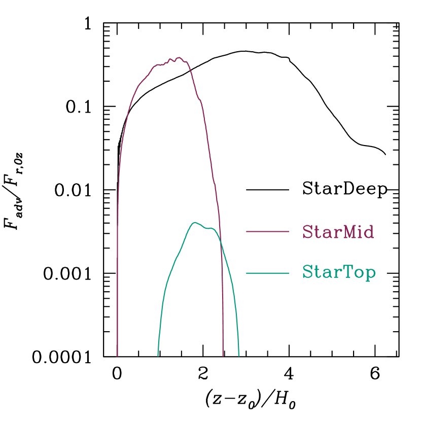
Figure 22.— Vertical profiles of the ratio between time averaged advection (convection) flux $F_{\rm adv}=v_{z}E_{r}$ and diffusive flux $F_{r,0z}$ for the three runs. Convection transports significant energy in StarDeep and in the deeper layers of StarMid. But in the outer layers of StarMid and throughout StarTop, photon diffusion is so rapid that it strongly suppresses the turbulent transport of energy.

We have presented three-dimensional (3D) radiation hydrodynamic simulations of the radiation pressure dominated envelopes of massive stars near the iron opacity peak. The resulting dynamics depends sensitively on the ratio of the photon diffusion time to the dynamical time. This is set by the ratio of the local optical depth $\tau_{0}$ to the critical optical depth $\tau_{c}=c/c_{g}$, where $c$ is the speed of light and $c_{g}$ is the isothermal sound speed. Our simulations cover the regimes $\tau_{0}\gg\tau_{c}$ (StarDeep), $\tau_{0}\sim\tau_{c}$ (StarMid), and $\tau_{0}\ll\tau_{c}$ (StarTop).

The iron opacity peak at $T\approx 1.6\times 10^{5}$ K leads to locally super-Eddington fluxes in the envelopes of massive stars. In radiative equilibrium this produces a pronounced density inversion in one-dimensional stellar models (Joss et al., 1973b; Paxton et al., 2013). The resulting density inversions are convectively unstable, but the properties of the resulting convection zones have until now been very uncertain when $\tau_{0}\lesssim\tau_{c}$ and convection is expected to be relatively inefficient.

Figures 21 and 22 compare the time and horizontally averaged turbulent properties of our three runs, showing the gas, radiation, and kinetic energy densities (Fig. 21) and the ratio of the convective and diffusive energy fluxes, respectively.

When $\tau_{0}\gg\tau_{c}$ as in StarDeep, convection is efficient and the averaged radiation advection flux is consistent with the convection flux as calculated using the MLT formalism (equation 17). We find that the mixing length parameter required to match the advection flux in the 3D simulation is $\alpha=0.55$, roughly consistent with the typical size of the turbulent structures $l_{\rho}/H_{0}\approx 0.3-0.4$ (as assumed in mixing length theory). The density inversion, present in the 1D radiative equilibrium initial condition, is absent in the turbulent state. This is because a significant fraction of the luminosity is transported by convection (Fig. 22), which reduces the radiation acceleration to be sub-Eddington. For StarDeep, the turbulent velocity is very subsonic with the turbulent kinetic energy less than $1\%$ of the thermal energy (Fig. 21). The difference between the actual thermal gradient $\nabla$ and the adiabatic gradient $\nabla_{\rm ad}$ is smaller than $8\%$ of $\nabla_{\rm ad}$. All of these properties are consistent with expectations for efficient convection.

When $\tau_{0}<\tau_{c}$, the advection flux drops significantly as photons cannot be trapped by the fluid due to rapid diffusion. We see this transition in the surface layers of run StarMid. As shown in Figure 12, below $60R_{\odot}$, the averaged radiation advection flux is consistent with MLT (eq. 17). The turbulent velocity is subsonic and $\tilde{\nabla}\ll 1$ as in StarDeep. However above $60R_{\odot}$, equation (17) significantly overpredicts the average convection flux if we use a constant $\alpha$, a choice motivated by the fact that the correlation length of the turbulence ($l_{\rho}/H_{0}$) is almost the same through the whole envelope. Above $60R_{\odot}$ the turbulent velocity reaches the isothermal sound speed and $\tilde{\nabla}$ increases significantly.

The run StarTop has $\tau_{0}\ll\tau_{c}$ and convection is very inefficient. In this case the average radiation advection flux is $\ll 1\%$ of the diffusive flux throughout the envelope (Figure 22). If we adopt the non-adiabatic MLT model (e.g., Henyey et al., 1965; Magic et al., 2015) with $\alpha=0.4$, which is the ratio of the turbulent correlation length to the pressure scale height, we find that it still significantly over-predicts the convection flux (Figure 18). The difference is probably caused by a combination of the porosity effect and vertical oscillation of the envelope as explained blow.

The turbulent velocity in StarTop is larger than the isothermal sound speed and strong shocks are formed, driving large density fluctuations. The bottom panel of Figure 21 shows, however, that the kinetic energy density only reaches the gas internal energy density, which is still much smaller than the radiation energy density. The large density fluctuations allow radiation to escape somewhat more efficiently (Shaviv, 1998) than through a homogenous medium (“porosity”), reducing the effective radiation acceleration. This effect is not, however, large enough to make the radiation acceleration smaller than the gravitational acceleration. The density inversion present in the initial conditions is initially destroyed by convection and the envelope expands, but the gas quickly falls back because of the reduced opacity and radiation acceleration. The density inversion then reforms. This cycle repeats, with the envelope undergoing strong vertical oscillations with a period of a few hours. The density inversion predicted by 1D radiative equilibrium models still exists in the time averaged vertical profile of StarTop, in contrast to StarDeep and StarMid where convection is able to largely eliminate the density inversion.

5.1. Observational consequences

A signature of inefficient convection is the appearance of supersonic turbulent velocities with respect to the isothermal sound speed (but not the radiation sound speed). This is because rapid diffusion leads the photons and gas to decouple and the radiation pressure cannot respond to density fluctuations. This in turn makes the gas highly compressible, leading to shocks and large density fluctuations.

In the calculations that include the photosphere (StarTop and StarMid) we observe turbulent velocities reaching the isothermal sound speed close to the stellar surface ($\approx 50$ km/s). These large velocities can impact the spectroscopic measurements of line profiles, as quantified by the macroturbulence (microturbulence) parameters. These parameters quantify the velocity fields at the stellar photosphere with correlation length larger (smaller) than the line-forming region. The extent of the line forming region is comparable to the local pressure scale-height, which is about the correlation length of the turbulent structures in our calculations. Therefore we expect the velocity fields observed in the simulations to potentially impact both micro- and macro- turbulence measurements. This is important, as the broadening of spectral lines is used to measure the (projected) rotational velocity of stars, which in the presence of extra turbulent broadening could be be systematically higher than the actual rotation rate (Ramírez-Agudelo et al., 2015). The idea that inefficient convection at the iron opacity peak could be responsible for the extra broadening of spectral lines in hot massive stars has been discussed previously (Cantiello et al., 2009), where they focused on the role of gravity waves excited by turbulent convection. Recently the potentially observable signature of turbulent pressure in the inefficient outer convective regions of massive stars has been highlighted by Grassitelli et al. (2015), who showed a correlation between observed macroturbulence and turbulent pressure (as calculated in the context of 1D MLT).

The vertical oscillations of the envelope in StarMid and StarTop also cause the radiation flux coming from the photosphere to vary with time. The standard deviations of the total radiation flux leaving from the photosphere are $\approx 13\%$ and $\approx 2.7\%$ of the time averaged mean values in StarMid and StarTop respectively. This means that this oscillation can be observed in principle. However, direct comparisons with observations require global calculations of the envelope.

Strange mode instabilities are commonly associated with opacity bumps and density inversions in 1D models of massive stars (e.g., Kiriakidis et al., 1993; Saio, 2009; Saio et al., 2013). These standing wave instabilities are fundamentally acoustic in nature, and are generally associated with a trapping region around the opacity bump/density inversion. The excitation mechanism of these modes is due to opacity variations in the acoustic wave, and is related to the growth mechanism of traveling acoustic waves discussed by Blaes & Socrates (2003). As we briefly noted above in section 4.3.1, conditions in StarTop at least are such that these traveling wave instabilities should be driven, and the fact that the density inversion persists in the time-averaged structure may permit the existence of trapped strange modes. It would be interesting to do a global stability analysis on the time-averaged structure of StarMid and StarDeep, to see if standing acoustic wave instabilities could still be trapped even in the absence of density inversions.

5.2. Implications for 1D stellar evolution

For $\tau_{0}\gtrsim\tau_{c}$, we find that mixing length theory provides a reasonable description of the convective energy transport in the 3D simulations. However, the mixing length parameters we find ($\alpha\approx 0.5$) are noticeably smaller than the canonically adopted values ($\alpha>1$, see e.g. Yusof et al., 2013; Köhler et al., 2015). We also find that as $\tau_{0}/\tau_{c}$ decreases, the mixing length parameter decreases. This is exactly the opposite of what has been proposed by different groups dealing with the numerical difficulties associated with radiation dominated stellar envelopes in 1D. They suggested that convection in this situation should be artificially enhanced (equivalent to increasing the $\alpha$ parameter with respect to the canonical values above), justifying this choice with either the need to remove an “unphysical density inversion” (Maeder, 1987; Ekström et al., 2012) or the need to include some (unknown) extra energy transport mechanism (Paxton et al., 2013).

Moreover we find that density inversions are present in the time averaged structure of the stellar envelope when $\tau_{0}\ll\tau_{c}$, i.e. when an opacity peak is close to the stellar surface. In the case of the iron opacity peak, this occurs for very massive main sequence stars, though we expect the same physics to occur in cooler objects due to the effect of the H and He opacity bumps (not studied in this work). The behavior of these density inversions is quite different as compared to the steady 1D solution, as they tend to be cyclically destroyed and reformed and are associated with very large density inhomogeneities. One important effect that is currently missing in the 1D models is the inclusion of a “porosity factor”, reducing the effective radiation acceleration when $\tau_{0}<\tau_{c}$ (e.g., Paczyński, 1969). The dependency of the porosity on optical depth, resolution and magnetic fields will be the focus of future work.

The turbulent, non-stationary behavior of radiation dominated envelopes suggests a possible modification of the stellar mass loss relative to spherically symmetric hydrostatic models (e.g., Owocki et al., 2004). Unfortunately as we only simulate a local patch of the envelope, we cannot determine the fate of the mass that leaves our simulation box. The mass loss rate also cannot be calculated self-consistently based on these simulations. This requires global calculations of the envelope to capture the change of gravitational acceleration and geometric dilution correctly.

The majority of massive stars are found in binary systems (Sana et al., 2012). Depending on their orbital separation and the evolution of their radii, these stars can fill their Roche lobe and strongly interact already during the main sequence (e.g., de Mink et al., 2014). As shown in this paper, the energy transport in the radiation dominated envelopes of these stars is not properly modeled in current 1D calculations, resulting in very uncertain values for the stellar radii. This could have important implications for the evolution of massive binaries and, for example, the predicted rates of BH-BH binary merges, which are promising sources of gravitational waves (Belczynski et al., 2014).

One limitation of the simulations presented here is that we have neglected the effects of the stellar magnetic field. Recently, magnetic buoyancy has been found to significantly enhance the radiation advection flux, even with a relatively weak magnetic field (Blaes et al., 2011; Jiang et al., 2014a). A fraction of massive stars do show significant magnetization (Wade et al., 2014), and dynamo generated magnetic fields could be present in the iron convection zone (Cantiello & Braithwaite, 2011). Therefore the effects of magnetic field should be studied in future work.

References

- Asplund et al. (2005) Asplund, M., Grevesse, N., & Sauval, A. J. 2005, 336, 25
- Belczynski et al. (2014) Belczynski, K., Buonanno, A., Cantiello, M., et al. 2014, ApJ, 789, 120
- Blaes et al. (2011) Blaes, O., Krolik, J. H., Hirose, S., & Shabaltas, N. 2011, ApJ, 733, 110
- Blaes & Socrates (2003) Blaes, O., & Socrates, A. 2003, ApJ, 596, 509
- Bromm & Larson (2004) Bromm, V., & Larson, R. B. 2004, ARA&A, 42, 79
- Cantiello & Braithwaite (2011) Cantiello, M., & Braithwaite, J. 2011, A&A, 534, A140
- Cantiello et al. (2009) Cantiello, M., Langer, N., Brott, I., et al. 2009, A&A, 499, 279
- Chandrasekhar (1967) Chandrasekhar, S. 1967, An introduction to the study of stellar structure
- Cox (1968) Cox, J. P. 1968, Principles of stellar structure - Vol.1: Physical principles; Vol.2: Applications to stars
- Crowther (2007) Crowther, P. A. 2007, ARA&A, 45, 177
- Davis et al. (2014) Davis, S. W., Jiang, Y.-F., Stone, J. M., & Murray, N. 2014, ApJ, 796, 107
- Davis et al. (2012) Davis, S. W., Stone, J. M., & Jiang, Y.-F. 2012, ApJS, 199, 9
- de Mink et al. (2014) de Mink, S. E., Sana, H., Langer, N., Izzard, R. G., & Schneider, F. R. N. 2014, ApJ, 782, 7
- Ekström et al. (2012) Ekström, S., Georgy, C., Eggenberger, P., et al. 2012, A&A, 537, A146
- Glatzel & Kiriakidis (1993) Glatzel, W., & Kiriakidis, M. 1993, MNRAS, 263, 375
- Glebbeek et al. (2009) Glebbeek, E., Gaburov, E., de Mink, S. E., Pols, O. R., & Zwart, S. F. P. 2009, Astronomy and Astrophysics, 497, 255
- Gräfener et al. (2012) Gräfener, G., Owocki, S. P., & Vink, J. S. 2012, A&A, 538, A40
- Grassitelli et al. (2015) Grassitelli, L., Fossati, L., Simon-Diaz, S., et al. 2015, arXiv:1507.03988
- Heger et al. (2003) Heger, A., Fryer, C. L., Woosley, S. E., Langer, N., & Hartmann, D. H. 2003, ApJ, 591, 288
- Henyey et al. (1965) Henyey, L., Vardya, M. S., & Bodenheimer, P. 1965, ApJ, 142, 841
- Herwig (2000) Herwig, F. 2000, A&A, 360, 952
- Iglesias & Rogers (1996) Iglesias, C. A., & Rogers, F. J. 1996, ApJ, 464, 943
- Jiang et al. (2013a) Jiang, Y.-F., Davis, S. W., & Stone, J. M. 2013a, ApJ, 763, 102
- Jiang et al. (2012) Jiang, Y.-F., Stone, J. M., & Davis, S. W. 2012, ApJS, 199, 14
- Jiang et al. (2013b) —. 2013b, ApJ, 778, 65
- Jiang et al. (2013c) —. 2013c, ApJ, 767, 148
- Jiang et al. (2014a) —. 2014a, ApJ, 796, 106
- Jiang et al. (2014b) —. 2014b, ApJ, 784, 169
- Joss et al. (1973a) Joss, P. C., Salpeter, E. E., & Ostriker, J. P. 1973a, ApJ, 181, 429
- Joss et al. (1973b) —. 1973b, ApJ, 181, 429
- Kennicutt (2005) Kennicutt, R. C. 2005, 227, 3
- Kiriakidis et al. (1993) Kiriakidis, M., Fricke, K. J., & Glatzel, W. 1993, MNRAS, 264, 50
- Köhler et al. (2015) Köhler, K., Langer, N., de Koter, A., et al. 2015, A&A, 573, A71
- Langer et al. (1985) Langer, N., El Eid, M. F., & Fricke, K. J. 1985, A&A, 145, 179
- Langer et al. (1983) Langer, N., Fricke, K. J., & Sugimoto, D. 1983, A&A, 126, 207
- Lowrie et al. (1999) Lowrie, R. B., Morel, J. E., & Hittinger, J. A. 1999, ApJ, 521, 432
- Maeder (1981) Maeder, A. 1981, A&A, 99, 97
- Maeder (1987) —. 1987, A&A, 173, 247
- Maeder (2009) —. 2009, Physics, Formation and Evolution of Rotating Stars
- Maeder et al. (2012) Maeder, A., Georgy, C., Meynet, G., & Ekström, S. 2012, A&A, 539, A110
- Magic et al. (2015) Magic, Z., Weiss, A., & Asplund, M. 2015, A&A, 573, A89
- Owocki (2015) Owocki, S. P. 2015, in Astrophysics and Space Science Library, Vol. 412, Astrophysics and Space Science Library, ed. J. S. Vink, 113
- Owocki et al. (2004) Owocki, S. P., Gayley, K. G., & Shaviv, N. J. 2004, ApJ, 616, 525
- Paczyński (1969) Paczyński, B. 1969, Acta Astronomica, 19, 1
- Paxton et al. (2011) Paxton, B., Bildsten, L., Dotter, A., et al. 2011, ApJS, 192, 3
- Paxton et al. (2013) Paxton, B., Cantiello, M., Arras, P., et al. 2013, ApJS, 208, 4
- Paxton et al. (2015) Paxton, B., Marchant, P., Schwab, J., et al. 2015, arXiv:1506.03146
- Proga et al. (2014) Proga, D., Jiang, Y.-F., Davis, S. W., Stone, J. M., & Smith, D. 2014, ApJ, 780, 51
- Puls et al. (2008) Puls, J., Vink, J. S., & Najarro, F. 2008, A&A Rev., 16, 209
- Ramírez-Agudelo et al. (2015) Ramírez-Agudelo, O. H., Sana, H., de Koter, A., et al. 2015, in IAU Symposium, Vol. 307, IAU Symposium, 76–81
- Saio (2009) Saio, H. 2009, Communications in Asteroseismology, 158, 245
- Saio et al. (2013) Saio, H., Georgy, C., & Meynet, G. 2013, MNRAS, 433, 1246
- Sana et al. (2012) Sana, H., de Mink, S. E., de Koter, A., et al. 2012, Science, 337, 444
- Sanyal et al. (2015) Sanyal, D., Grassitelli, L., Langer, N., & Bestenlehner, J. M. 2015, arXiv:1506.02997
- Shaviv (1998) Shaviv, N. J. 1998, ApJ, 494, L193
- Smith (2014) Smith, N. 2014, ARA&A, 52, 487
- Stone et al. (2008) Stone, J. M., Gardiner, T. A., Teuben, P., Hawley, J. F., & Simon, J. B. 2008, ApJS, 178, 137
- Stothers & Chin (1979) Stothers, R., & Chin, C.-W. 1979, ApJ, 233, 267
- Suárez-Madrigal et al. (2013) Suárez-Madrigal, A., Krumholz, M., & Ramirez-Ruiz, E. 2013, arXiv:1304.2317
- Tsang & Milosavljevic (2015) Tsang, B. T.-H., & Milosavljevic, M. 2015, arXiv:1506.05121
- Turner et al. (2003) Turner, N. J., Stone, J. M., Krolik, J. H., & Sano, T. 2003, ApJ, 593, 992
- van Marle et al. (2008) van Marle, A. J., Owocki, S. P., & Shaviv, N. J. 2008, MNRAS, 389, 1353
- Wade et al. (2014) Wade, G. A., Grunhut, J., Alecian, E., et al. 2014, in IAU Symposium, Vol. 302, IAU Symposium, 265–269
- Yusof et al. (2013) Yusof, N., Hirschi, R., Meynet, G., et al. 2013, MNRAS, 433, 1114