Permuting Longitudinal Data Despite All The Dependencies

Abstract

For general repeated measures designs the Wald-type statistic (WTS) is an asymptotically valid procedure allowing for unequal covariance matrices and possibly non-normal multivariate observations. The drawback of this procedure is the poor performance for small to moderate samples, i.e., decisions based on the WTS may become quite liberal. It is the aim of the present paper to improve its small sample behavior by means of a novel permutation procedure. In particular, it is shown that a permutation version of the WTS inherits its good large sample properties while yielding a very accurate finite sample control of the type-I error as shown in extensive simulations. Moreover, the new permutation method is motivated by a practical data set of a split plot design with a factorial structure on the repeated measures.

Abstract

In this supplementary material to the authors’ paper ’Permuting longitudinal data despite all the dependencies’ we present all technical details together with additional simulation results and consider further resampling techniques, namely a nonparametric and a parametric bootstrap approach. Furthermore, we analyze the power of the WTPS and compare it to the power of the ATS. Finally, we present more details about the the data example on $O_{2}$-consumption of leukocytes and also present an analysis, where we applied all considered approaches.

Keywords: Permutation Tests; Longitudinal Data; Quadratic Forms; Repeated Measures.

^∗ University of Ulm, Institute of Statistics, Germany
  email: sarah.friedrich@uni-ulm.de

^∗∗ University Medical Center Göttingen, Institute of Medical Statistics, Germany

1 Motivation and Introduction

In many experiments in the life, social or psychological sciences the experimental units (e.g. subjects) are repeatedly observed at different occasions (e.g. at different time points) or under different treatment conditions. This leads to certain dependencies between observations from the same unit and results in a more complicated statistical analysis of such studies. In the context of experimental designs, the repeated measures are considered as levels of the sub-plot factor. If several groups are observed, these are considered as levels of the whole-plot factor. Typical questions in this setting concern the investigation of a group effect, a non-constant effect of time or different time profiles in the groups. Classical repeated measures models, where hypotheses are tested with Hotelling’s $T^{2}$ (Hotelling, 1931) or Wilks’s $\Lambda$ (Wilks, 1932), assume normally distributed observation vectors and a common covariance matrix for all groups, see e.g. the monograph of Davis (2002). In medical and biological research, however, the assumptions of equal covariance matrices and multivariate normally distributed outcomes are often not met and a violation of them may inflate the type-I error rates, see the comments in Xu and Cui (2008), Suo et al. (2013) or Konietschke et al. (2015). Therefore, other procedures have been developed for repeated measures which are based on certain approximation techniques (Geisser and Greenhouse (1958); Greenhouse and Geisser (1959); Huynh and Feldt (1976); Lecoutre (1991); Keselman et al. (2000); Werner (2004); Ahmad et al. (2008); Brunner (2009); Brunner et al. (2009); Kenward and Roger (2009); Brunner et al. (2012); Chi et al. (2012); Pauly et al. (2015b)). However, these papers mainly assume the multivariate normal distribution and only discuss methods for specific models which are also asymptotically only approximations, i.e., they do not even lead to asymptotic exact tests. Another possibility is to apply a specific mixed model in the GEE context, see e.g. the text books by Verbeke and Molenberghs (2009, 2012). These methods require that the data stems from a specific exponential family. An exception is given by the multivariate Wald-type test statistic (WTS) which is asymptotically exact. However, it is well known that it requires large sample sizes to keep the pre-assigned type-I error level, see e.g. Brunner (2001), Pauly et al. (2015a) and Konietschke et al. (2015).
To improve the small sample behavior of the WTS in a MANOVA setting, Konietschke et al. (2015) proposed different bootstrap techniques. Another possibility would be to apply permutation procedures. It is well known that permutation tests are finitely exact under the assumption of exchangeability, see e.g. Brombin et al. (2013), Pesarin (2001), Mielke and Berry (2007) or Pesarin and Salmaso (2010a, b, 2012) for examples. In most of these examples, however, permutation tests are only applied in situations where the null distribution is invariant under the corresponding randomization group. A modified permutation procedure may also be applied in situations where this invariance does not hold, see e.g. Janssen and Pauls (2003), Janssen (2005), Omelka and Pauly (2012), Chung and Romano (2013) and Pauly et al. (2015a). The main idea in these papers is to apply a studentized test statistic and to use its permutation distribution (based on permuting the pooled sample) for calculating critical values. This leads to particularly good finite sample properties even in case of general factorial designs with fixed factors, see Pauly et al. (2015a). It is the aim of the present paper to extend the concept of permuting all data to the context of longitudinal data in general (not necessarily normal and homoscedastic) split plot designs. Applied to the WTS this generalizes the results of Pauly et al. (2015a) and leads to astonishingly accurate results despite the dependencies in repeated measurements data.

The methodology derived in this paper is motivated by the following data example on the $O_{2}$ consumption of leukocytes. To examine the breathability of leukocytes, an experiment with 44 HSD-rats was conducted. A group of 22 rats was treated with a placebo, while the other 22 rats were treated with a substance supposed to enhance the humoral immunity. 18 hours prior to the opening of the abdominal cavity, all animals received 2.4 g sodium-caseinat for the production of a peritoneal exudate rich on leukocytes. In order to obtain a sufficient amount of material the peritoneal liquid of 3–4 animals was mixed and the leukocytes therein were rehashed in an experimental batch. One half of the experimental batch was mixed with inactivated staphylococci in a ratio of 100:1, the other half remained untreated and served as a control. Then, the oxygen consumption of the leukocytes was measured with a polarographic electrode after 6, 12 and 18 minutes, respectively. For each group separately, 12 experimental batches were carried out. The means over the experimental batches in both treatment groups are listed in Table 1.

Table 1: Mean oxygen consumption of leukocytes in the presence and absence of inactivated staphylococci.

Mean $O_{2}$-Consumption [$\mu\ell$]
	Staphylococci
	With			Without
	Time [min]			Time [min]
	6	12	18	6	12	18
Placebo	1.618	2.434	3.527	1.322	2.430	3.425
Verum	1.656	2.799	4.029	1.394	2.57	3.677

Questions of interest in this example concern the effect of the whole-plot factor ’treatment’, the effect of the sub-plot factors ’staphylococci’ and ’time’ as well as interactions between these effects. We note that the empirical $6\times 6$ covariance matrices of the two groups appear to be quite different (see the supplement for details). This also motivates to include unequal covariance matrices in our model. For such experimental designs procedures are derived in this paper that lead to good small sample control of the type-I error while being asymptotically exact.

The paper is organized as follows. The underlying statistical model is described in Section 2, where we also introduce the Wald-type (WTS) as well as the ANOVA-type statistic (ATS) and state their asymptotic behavior. In Section 3, we describe the novel permutation procedure used to improve the small sample behavior of the WTS. Afterwards, we present the results of extensive simulation studies in Section 4, analyzing the behavior of the permuted test statistic in different simulation designs with certain competitors. Additional simulation results have also been run for several other resampling schemes. They did not show a better performance than the permutation procedure and are only reported in the supplementary material, where also various power simulations can be found. The motivating data example is analyzed in detail in Section 5. The paper closes with a brief discussion of our results in Section 6. All proofs are given in the supplementary material.

2 Statistical Model, Hypotheses and Statistics

2.1 Statistical Model and Hypotheses

To establish the general model, let

$$\boldsymbol{Y}_{ik} = (Y_{ik1},\dots,Y_{ikt_{i}})^{\prime},\hskip 14.22636pti=1,\dots,a;\;\;k=1,\dots,n_{i}$$ (2.1)

denote independent random vectors with distribution $F_{i}$, expectation $\boldsymbol{\mu}_{i}=(\mu_{i1},\dots,\mu_{it_{i}})^{\prime}=E(\boldsymbol{Y}_{i1})$ and covariance matrix $\boldsymbol{V}_{i}=\operatorname{{\it Cov}}(\boldsymbol{Y}_{i1})>0$ in treatment group $i$. We do not assume any special structure of the covariance matrix $\boldsymbol{V}_{i}$ which may even be different between groups $1\leq i\leq a$. Note that we also allow the number of time points $t_{i}$ to differ between groups. The most common case where $t_{i}=t$ for all $i=1,\dots,a$ is thus a special case of model (2.1). Here the time points $t_{i}\in\mathbb{N}$ are fixed. For convenience, we collect the observation vectors $\boldsymbol{Y}_{ik}$ in

$$\boldsymbol{Y} = (\boldsymbol{Y}_{1}^{\prime},\dots,\boldsymbol{Y}_{a}^{\prime})^{\prime},\hskip 28.45274pt\boldsymbol{Y}_{i}=(\boldsymbol{Y}_{i1}^{\prime},\dots,\boldsymbol{Y}_{in_{i}}^{\prime})^{\prime}.$$ (2.2)

In this set-up, hypotheses are formulated as $H_{0}^{\mu}:\boldsymbol{H}\boldsymbol{\mu}=\boldsymbol{0}$, where $\boldsymbol{\mu}=(\boldsymbol{\mu}_{1}^{\prime},\dots,\boldsymbol{\mu}_{a}^{\prime})^{\prime}$ denotes the vector of all expectations $\mu_{is}=E(Y_{i1s})$, $i=1,\dots,a;\;s=1,\dots,t_{i}$ and $\boldsymbol{H}$ is a suitable contrast matrix, i.e., its rows sum up to zero. Examples of $\boldsymbol{H}$ are presented in Section 4.

Throughout the paper, we will use the following notation. We denote by $\boldsymbol{I}_{t}$ the $t$-dimensional unit matrix and by $\boldsymbol{J}_{t}$ the $t\times t$ matrix of 1’s, i.e., $\boldsymbol{J}_{t}=\boldsymbol{1}_{t}\boldsymbol{1}_{t}^{\prime}$, where $\boldsymbol{1}_{t}=(1,\dots,1)^{\prime}$ is the $t$-dimensional column vector of 1’s. Furthermore, let $\boldsymbol{P}_{t}=\boldsymbol{I}_{t}-\frac{1}{t}\boldsymbol{J}_{t}$ denote the $t$-dimensional centering matrix. By $\oplus$ and $\otimes$ we denote the direct sum and the Kronecker product, respectively.

An estimator of $\boldsymbol{\mu}$ is given by

$$\boldsymbol{\overline{Y}}_{\cdot}=(\boldsymbol{\overline{Y}}_{1\cdot}^{\prime},\dots,\boldsymbol{\overline{Y}}_{a\cdot}^{\prime})^{\prime}\text{ for }\boldsymbol{\overline{Y}}_{i\cdot}=(Y_{i\cdot 1},\dots,Y_{i\cdot t_{i}})^{\prime},~{}\overline{Y}_{i\cdot s}=\frac{1}{n_{i}}\sum_{k=1}^{n_{i}}{Y_{iks}},~{}s=1,\dots,t_{i}$$

and the covariance matrix $\boldsymbol{V}_{i}$ in treatment group $i$ is estimated by the sample covariance matrix

$$\boldsymbol{\widehat{V}}_{i}=\frac{1}{n_{i}-1}\sum_{k=1}^{n_{i}}(\boldsymbol{Y}_{ik}-\boldsymbol{\overline{Y}}_{i\cdot})(\boldsymbol{Y}_{ik}-\boldsymbol{\overline{Y}}_{i\cdot})^{\prime},~{}i=1,\dots,a.$$

Let $N=\sum_{i=1}^{a}n_{i}$ denote the total number of subjects in the trial, $T=\sum_{i=1}^{a}t_{i}$ the total number of time points and $\tilde{N}=\sum_{i=1}^{a}n_{i}t_{i}$ the total number of observations. Then the asymptotic results are derived under the following two assumptions:

• $\frac{n_{i}}{N}\to\kappa_{i}\in(0,1)$ as $\min(n_{1},\ldots,n_{a})\to\infty$,

• $\sup_{i}E(||\boldsymbol{Y}_{i1}||^{4})<\infty$.

2.2 Statistics and Asymptotics

We consider two commonly used test statistics for repeated measures and multivariate data. First, the so-called ANOVA-type statistic (ATS), introduced in Brunner (2001), is given as:

$$\widetilde{Q}_{N}=N\boldsymbol{\overline{Y}}_{\cdot}^{\prime}\boldsymbol{H}^{\prime}(\boldsymbol{H}\boldsymbol{H}^{\prime})^{-}\boldsymbol{H}\boldsymbol{\overline{Y}}_{\cdot}=N\boldsymbol{\overline{Y}}_{\cdot}^{\prime}\boldsymbol{T}\boldsymbol{\overline{Y}}_{\cdot},$$ (2.3)

where $(\cdot)^{-}$ denotes some generalized inverse. Note that the test statistic does not depend on the special choice of the generalized inverse. Its asymptotic distribution is established in the next theorem.

Theorem 2.1

Under the null hypothesis $H_{0}^{\mu}:\boldsymbol{H}\boldsymbol{\mu}=\boldsymbol{0}$, the ATS in (2.3) has, asymptotically, the same distribution as the random variable

$$X=\sum_{i=1}^{a}\sum_{s=1}^{t_{i}}\lambda_{is}X_{is},$$

where $X_{is}\stackrel{{\scriptstyle i.i.d.}}{{\sim}}\chi_{1}^{2}$ and the weights $\lambda_{is}$ are the eigenvalues of $\boldsymbol{T}\boldsymbol{\Sigma}$ for $\boldsymbol{\Sigma}=\bigoplus_{i=1}^{a}\kappa_{i}^{-1}\boldsymbol{V}_{i}$.
Moreover, for local alternatives $\boldsymbol{T}\boldsymbol{\mu}=\frac{1}{\sqrt{N}}\cdot\boldsymbol{T}\boldsymbol{\nu},\boldsymbol{\nu}\in\mathbb{R}^{T}$, it holds that the ATS has, asymptotically, the same distribution as $\boldsymbol{Z}^{\prime}\boldsymbol{T}\boldsymbol{Z}$, where $\boldsymbol{Z}\sim N(\boldsymbol{\nu},\boldsymbol{\Sigma})$. If additionally $\boldsymbol{\Sigma}>0$, the ATS has the same distribution as a weighted sum of $\chi^{2}_{1}(\delta)$ distributed random variables, where the weights are again the eigenvalues $\lambda_{is}$ and $\delta=\boldsymbol{\nu}^{\prime}\boldsymbol{\Sigma}^{-1}\boldsymbol{\nu}$.

Since the $\lambda_{is}$ are unknown, the result cannot be applied directly. Nevertheless, Brunner (2001) proposed to approximate the distribution of $X$ by the distribution of a scaled $\chi^{2}$-distribution, i.e., by $g\cdot\tilde{X}_{\nu}$, where $\tilde{X}_{\nu}\sim\chi^{2}_{\nu}$ (Box, 1954). The constants $g$ and $\nu$ are estimated from the data such that the first two moments of $X$ and $g\cdot\tilde{X}_{\nu}$ coincide (Box, 1954). This leads to approximating the statistic

$$F_{N}=\frac{N}{\operatorname{tr}(\boldsymbol{T}\boldsymbol{\widehat{\Sigma}})}\boldsymbol{\overline{Y}}_{\cdot}^{\prime}\boldsymbol{T}\boldsymbol{\overline{Y}}_{\cdot}$$ (2.4)

by an $F(\widehat{\nu},\infty)$-distribution with estimated degree of freedom $\hat{\nu}=\operatorname{tr}^{2}(\boldsymbol{T}\boldsymbol{\widehat{\Sigma}})/\operatorname{tr}(\boldsymbol{T}\boldsymbol{\widehat{\Sigma}})^{2}$, where $\boldsymbol{\widehat{\Sigma}}=N\bigoplus_{i=1}^{a}\frac{1}{n_{i}}\boldsymbol{\widehat{V}}_{i}$. The corresponding ATS test $\varphi_{ATS}={\mathds{1}}\{\widetilde{Q}_{N}>F_{\alpha}(\widehat{\nu},\infty)\}$, where $F_{\alpha}(\widehat{\nu},\infty)$ denotes the $(1-\alpha)$-quantile of the $F(\widehat{\nu},\infty)$-distribution, leads to consistent test decisions for fixed alternatives. However, it is in general no asymptotic level $\alpha$ test under the null hypothesis, which is a severe drawback of this procedure. Thus, we discuss a second statistic, the so-called Wald-type statistic (WTS) given as

$$Q_{N}=N\boldsymbol{\overline{Y}}_{\cdot}^{\prime}\boldsymbol{H}^{\prime}(\boldsymbol{H}\boldsymbol{\widehat{\Sigma}}\boldsymbol{H}^{\prime})^{+}\boldsymbol{H}\boldsymbol{\overline{Y}}_{\cdot}.$$ (2.5)

Here $(\boldsymbol{H}\boldsymbol{\widehat{\Sigma}}\boldsymbol{H}^{\prime})^{+}$ denotes the Moore-Penrose inverse of $(\boldsymbol{H}\boldsymbol{\widehat{\Sigma}}\boldsymbol{H}^{\prime})$. In order to test the general linear hypotheses $H_{0}^{\mu}:\boldsymbol{H}\boldsymbol{\mu}={\bf 0}$ critical values are taken from the asymptotic distribution of $Q_{N}$ under the null hypothesis stated below.

Theorem 2.2

Under the null hypothesis $H_{0}^{\mu}:\boldsymbol{H}\boldsymbol{\mu}=\boldsymbol{0}$, the WTS in (2.5) has, asymptotically, a central $\chi^{2}_{f}$-distribution with $f=\operatorname{\it rank}(\boldsymbol{H})$. The corresponding test is given by $\varphi_{WTS}={\mathds{1}}\{Q_{N}>\chi^{2}_{f,1-\alpha}\}$, where $\chi^{2}_{f,1-\alpha}$ denotes the $(1-\alpha)$-quantile of the $\chi^{2}_{f}$ distribution. This test is an asymptotic level $\alpha$ test and is consistent for general fixed alternatives $\boldsymbol{H}\boldsymbol{\mu}\neq{\bf 0}$. Moreover, for local alternatives $\boldsymbol{H}\boldsymbol{\mu}=\frac{1}{\sqrt{N}}\cdot\boldsymbol{\nu},\boldsymbol{\nu}\in\mathbb{R}^{T}$, it holds that $Q_{N}$ has asymptotically a non-central $\chi^{2}_{f}(\tilde{\delta})$ distribution where $\tilde{\delta}=(\boldsymbol{H}\boldsymbol{\nu})^{\prime}(\boldsymbol{H}\boldsymbol{\Sigma}\boldsymbol{H}^{\prime})^{+}\boldsymbol{H}\boldsymbol{\nu}$. This implies that $E_{H_{1}}(\varphi_{WTS})\to P(Z>\chi^{2}_{f,1-\alpha})$ with $Z\sim\chi^{2}_{f}(\tilde{\delta})$.

Although $\varphi_{WTS}$ possesses these nice asymptotic properties, it is well-known that very large sample sizes $n_{i}$ are necessary to maintain the pre-assigned level $\alpha$ using quantiles of the limiting $\chi^{2}$-distribution, see Konietschke et al. (2015), Pauly et al. (2015a) and Brunner (2001) as well as Table 2 below. This leads to a limited applicability of the WTS in practice.

To accept the need for a novel procedure, we investigate the accuracy of the two test statistics in a one sample repeated measure design with $n$ subjects and $t$ repeated measures $Y_{ks}$. The null hypothesis $H_{0}^{\mu}:\{\mu_{1}=\dots=\mu_{t}\}=\{\boldsymbol{P}_{t}\boldsymbol{\mu}={\bf 0}\},\boldsymbol{\mu}=(\mu_{1},\dots,\mu_{t})^{\prime}$ is considered and the components of $\boldsymbol{Y}_{k}$ are selected as standardized log-normally distributed random variables, i.e.,

$$Y_{ks}=\frac{{\epsilon}_{ks}-E({\epsilon}_{ks})}{\sqrt{\operatorname{{\it Var}}({\epsilon}_{ks})}}$$

for i.i.d. log-normally distributed ${\epsilon}_{ks}$, $k=1,\dots,n$ and $s=1,\dots,t$. The results are displayed in Table 2, where the simulated type-I error rates of the WTS and ATS are given. It is readily seen that the test based on the WTS considerably exceeds the nominal level of 5%, while the ATS leads to rather conservative decisions.

Table 2: Simulated type-I error rates (10000 simulations) in a repeated measures design with $n=10,20,50,100$ individuals and $t=4,8$ repeated measures. The ATS is compared to the upper 5% quantile of the $F(\hat{\nu},\infty)$-distribution, the WTS to the upper 5% quantile of the $\chi^{2}_{t-1}$-distribution.

	Type-I error rates ($\alpha=0.05$)
	ATS: F-quantile		WTS: $\chi^{2}$-quantile
$n$	$t=4$	$t=8$	$t=4$	$t=8$
10	0.025	0.012	0.223	0.776
20	0.026	0.014	0.126	0.388
50	0.030	0.021	0.081	0.166
100	0.035	0.025	0.067	0.111

Thus, to enhance the small sample properties of the above tests we have compared different resampling approaches in an extensive simulation study, presented in Section 9 of the supplementary material Friedrich et al. (2016). Surprisingly, the best procedure turned out to be a permutation technique that randomly permutes the pooled univariate observations without taking into account the existing dependencies for calculating critical values. This at first sight counter-intuitive method is motivated from Konietschke and Pauly (2014), where a similar approach has been applied in the paired two-sample case. Moreover, the current procedure generalizes the permutation test on independent observations by Pauly et al. (2015a) and implemented in the R package GFD (Friedrich et al., 2015) to the case of repeated measures and multivariate data. The details are explained in the next section.

3 The Permutation Procedure

Let $\boldsymbol{Y}^{\pi}=\pi(Y_{111},\cdots,Y_{an_{a}t_{a}})^{\prime}=(Y_{111}^{\pi},\cdots,Y_{an_{a}t_{a}}^{\pi})^{\prime}$ denote a fixed but arbitrary permutation of all $\tilde{N}$ elements of $\boldsymbol{Y}$ in (2.2), i.e., $\pi\in\mathcal{S}_{\tilde{N}}$. In this notation, $Y_{iks}^{\pi}$ denotes the $(i,k,s)-$component of the permuted vector $\boldsymbol{Y}$. Furthermore, let $\boldsymbol{\overline{Y}}_{\cdot}^{\pi}$ denote the vector of the means under this permutation and $\boldsymbol{\widehat{\Sigma}}^{\pi}=\bigoplus_{i=1}^{a}\frac{N}{n_{i}}\boldsymbol{\widehat{V}}_{i}^{\pi}$ the empirical covariance matrix of the permuted observations.

It is obvious, that $\boldsymbol{Y}$ and $\boldsymbol{Y}^{\pi}$ only have the same distribution, if the components of $\boldsymbol{Y}$ are exchangeable. However, this is not the case in general two- and higher way layouts, even in the case of independent observations, see e.g. Huang et al. (2006). Following the approach of Neuhaus (1993), Janssen (1997, 2005), Omelka and Pauly (2012), Chung and Romano (2013) and Pauly et al. (2015a) in the case of independent observations, the idea is to studentize the statistic $\sqrt{N}\boldsymbol{\overline{Y}}_{\cdot}^{\pi}$ and consider its projection into the hypothesis space, resulting in the WTS of the permuted observations, namely

$$Q_{N}^{\pi}=N(\boldsymbol{\overline{Y}}_{\cdot}^{\pi})^{\prime}\boldsymbol{H}^{\prime}(\boldsymbol{H}\boldsymbol{\widehat{\Sigma}}^{\pi}\boldsymbol{H}^{\prime})^{+}\boldsymbol{H}\boldsymbol{\overline{Y}}_{\cdot}^{\pi}.$$ (3.1)

In the sequel we will denote $Q_{N}^{\pi}$ as the WTPS. Note, that the question how to permute is more involved here than in the case of independent univariate observations. A heuristic reason why the above approach might work is as follows: Unconditionally, all permuted components possess the same mean. Thus, when multiplied by a contrast matrix the permuted means vector always mimics the null situation, i.e., $\boldsymbol{H}E(\boldsymbol{\overline{Y}}_{\cdot}^{\pi})={\bf 0}$ always holds. In particular, it can be shown that the conditional distribution of the WTPS $Q_{N}^{\pi}$ in (3.1) always approximates the null distribution of $Q_{N}$ in (2.5) in the general repeated measures design under study; thus leading to an asymptotically valid permutation test. This result is formulated in the following theorem:

Theorem 3.1

The studentized permutation distribution of $Q_{N}^{\pi}$ in (3.1) conditioned on the observed data $\boldsymbol{Y}$ weakly converges to the central $\chi^{2}_{f}$ distribution in probability, where $f=rank(\boldsymbol{H})$.

Remark 3.1

Theorem 3.1 states that the permutation distribution asymptotically provides a valid approximation of the null distribution of the test statistic $Q_{N}$ in (2.5). To be concrete, this means that for any underlying parameters $\boldsymbol{\mu}\in\mathbb{R}^{T}$ and $\boldsymbol{\mu}_{0}\in H_{0}(\boldsymbol{H})$ with $\boldsymbol{H}\boldsymbol{\mu}_{0}={\bf 0}$ we have convergence in probability

$$\sup_{x\in\mathbb{R}}\left|P_{\boldsymbol{\mu}}(Q_{N}^{\pi}\leq x|\boldsymbol{Y})-P_{\boldsymbol{\mu}_{0}}(Q_{N}\leq x)\right|\to 0.$$ (3.2)

Here, $P_{\boldsymbol{\mu}}(Q_{N}\leq x)$ and $P_{\boldsymbol{\mu}}(Q_{N}^{\pi}\leq x|\boldsymbol{Y})$ denote the unconditional and conditional distribution function of $Q_{N}$ and $Q_{N}^{\pi}$, respectively, under the assumption that $\boldsymbol{\mu}$ is the true underlying parameter.

Remark 3.2

A Wald-type permutation test is obtained by comparing the original test statistic $Q_{N}$ with the $(1-\alpha)$-quantile $c^{*}_{1-\alpha}$ of the conditional distribution of the WTPS $Q_{N}^{\pi}$ given the observed data $\boldsymbol{Y}$, i.e., $\varphi_{WTPS}={\mathds{1}}\{Q_{N}>c^{*}_{1-\alpha}\}$. Theorem 3.1 implies that this test asymptotically keeps the pre-assigned level $\alpha$ under the null hypothesis and is consistent for any fixed alternative $\boldsymbol{H}\boldsymbol{\mu}\neq\textbf{0}$, i.e., it has asymptotically power 1. Moreover, it has the same asymptotic power as the WTS for local alternatives $\boldsymbol{H}\boldsymbol{\mu}=\frac{1}{\sqrt{N}}\cdot\boldsymbol{\nu}$, i.e., it holds that $E_{H_{1}}(\varphi_{WTPS})\to P(Z>\chi^{2}_{f,1-\alpha})$ with $Z\sim\chi^{2}_{f}(\tilde{\delta})$ as in Theorem 2.2.

It follows that the permutation test and the classical Wald-type test are asymptotically equivalent and that both have the same local power under contiguous alternatives. In particular the asymptotic relative efficiency of the WTPS compared to the classical WTS is 1. Moreover, the permutation test based on $Q_{N}^{\pi}$ is finitely exact if the pooled data $\boldsymbol{Y}$ are exchangeable under the null hypothesis. In comparison, the ATS also leads to a consistent test for fixed alternatives but does not provide an asymptotic level $\alpha$ test since it is only an approximation.

We note, that the proof given in the supplement to this paper indicates that the given permutation technique does not work in case of the ATS. In particular, a permutation version of the ATS would also possess a weighted $\chi^{2}$-limit distribution but with different weights, say $\tilde{\lambda}_{is}$, due to an incorrect covariance structure.

Remark 3.3

Our general framework (2.1) allows for the treatment of different important factorial designs in the context of multivariate repeated measures data analysis. As in Pauly et al. (2015a) the idea is to accordingly split the indices in subindices and to choose an appropriate hypothesis matrix $\boldsymbol{H}$. Examples of different cross-classified and hierarchically nested designs are discussed in Section 4 of Konietschke et al. (2015). For repeated measures, examples are given in Sections 4 and 5 below as well as in Brunner (2001).

4 Simulations

In order to investigate the small sample behavior of the WTPS, we present extensive simulation results for different designs and covariance structures. The procedure is analyzed in different settings with regard to maintaining the pre-assigned type-I error rate ($\alpha=5\%$). The results for the WTPS are compared to the asymptotic quantiles of the ATS ($F$-quantile) and the WTS ($\chi^{2}$-quantile).

4.1 Data Generation

For our simulation studies, we simulated a split plot design which, in the context of longitudinal data, is a design with $a$ groups, $n_{i}$ subjects in group $i$ and $t_{i}=t$ repeated measures $Y_{iks},s=1,\dots,t$. Let

$$\boldsymbol{Y}_{ik}=(Y_{ik1},\ldots,Y_{ikt})^{\prime}=\boldsymbol{\mu}_{i}+B_{ik}{\bf 1}_{t}+\boldsymbol{V}_{i}^{1/2}\boldsymbol{\epsilon}_{ik},$$

with $\boldsymbol{\mu}_{i}=E(\boldsymbol{Y}_{i1}),i=1,\dots,a,$ and let $B_{ik}\sim N(0,\sigma_{i}^{2})$ denote independent additive subject effects. The i.i.d. random vectors $\boldsymbol{\epsilon}_{ik}=(\epsilon_{ik1},\dots,\epsilon_{ikt})$ were generated from different standardized distributions by

$$\epsilon_{iks}=\frac{\tilde{\epsilon}_{iks}-E(\tilde{\epsilon}_{iks})}{\sqrt{\operatorname{{\it Var}}(\tilde{\epsilon}_{iks})}},$$

where $\tilde{\epsilon}_{iks}$ denote i.i.d. normal, exponential or log-normal random variables.

A simulation setting with $a=3$ groups and $t=4,8$ repeated measures was considered. The null hypotheses investigated are

1. The hypothesis of no time effect $T$

   $$H_{0}^{\mu}(T) : \overline{\mu}_{\cdot 1}=\dots=\overline{\mu}_{\cdot t}\quad\text{or equivalently}\quad\boldsymbol{H}_{T}\boldsymbol{\mu}=\boldsymbol{0},$$

2. The hypothesis of no group $\times$ time interaction effect $GT$

   $$H_{0}^{\mu}(GT) : \boldsymbol{H}_{GT}\boldsymbol{\mu}=\left(\begin{array}[]{l}\mu_{11}-\overline{\mu}_{1\cdot}-\overline{\mu}_{\cdot 1}+\overline{\mu}_{\cdot\cdot}\\ \vdots\\ \mu_{at}-\overline{\mu}_{a\cdot}-\overline{\mu}_{\cdot t}+\overline{\mu}_{\cdot\cdot}\end{array}\right)=\boldsymbol{0},$$

   where $\boldsymbol{H}_{T}=\frac{1}{a}\boldsymbol{1}_{a}^{\prime}\otimes\boldsymbol{P}_{t}$ and $\boldsymbol{H}_{GT}=\boldsymbol{P}_{a}\otimes\boldsymbol{P}_{t}.$

We considered balanced as well as unbalanced designs for the $\boldsymbol{n}=(n_{1},n_{2},n_{3})$ subjects in group 1–3, respectively. The simulated numbers of subjects were $\boldsymbol{n}^{(1)}=(30,20,10),\,\boldsymbol{n}^{(2)}=(10,20,30)$ and $\boldsymbol{n}^{(3)}=(15,15,15)$. Furthermore, we simulated three different covariance structures $\boldsymbol{V}_{i}$

• Setting 1: $\boldsymbol{V}_{i}=\boldsymbol{I}_{t}$ for all $i=1,2,3$

• Setting 2: $\boldsymbol{V}_{i}=diag(\sigma_{1}^{2},\dots,\sigma_{t}^{2})$ with $\sigma_{s}^{2}=s$ for $t=4$ and $\sigma_{s}^{2}=\sqrt{s}$ for $t=8$

• Setting 3: $\boldsymbol{V}_{i}=\left(\rho_{i}^{|l-j|}\right)_{l,j\leq t},(\rho_{1},\rho_{2},\rho_{3})=(0.6,0.5,0.4)$ for $i=1,2,3$

In Setting 1 and 2 the covariance structures are the same for all groups, whereas in Setting 3 we have an autoregressive covariance structure with different parameters for the different groups. Moreover, we simulated block effects with different variances $\sigma_{i}^{2}\in\{0,1,2\}$. However, since the results were almost identical, we here only report the case $\sigma_{i}^{2}=0$. All simulations were conducted with 10,000 simulation and 1,000 permutation runs.

4.2 Type-I error rates

The resulting type-I error rates for the hypotheses of no time effect $T$ and no group $\times$ time interaction $GT$ are displayed in Tables 3 and 4, respectively.

It is obvious that the tests based on the WTS considerably exceed the nominal level for small sample sizes. This behavior becomes worse with an increasing number of repeated measurements and when testing the interaction hypothesis. In some cases, the WTS reaches an empirical type-I error rate of almost 50% when testing the $GT$-interaction. This means that its accuracy is no better than flipping a coin. The ATS, in contrast, keeps the pre-assigned level $\alpha$ pretty well for normally distributed observations, even for small sample sizes. With an increasing number of repeated measurements and/or non-normal data, however, the ATS leads to quite conservative decisions. Furthermore, the ATS leads to slightly conservative decisions when testing the interaction hypothesis, even with normally distributed data. The WTPS is reasonably close to the pre-assigned level $\alpha$ in most situations, even under non-normality and for testing the interaction hypothesis. Despite the dependencies in longitudinal data, the permutation procedure greatly improves the behavior of the WTS in small sample settings. However, when testing the interaction hypothesis for $t=8$ repeated measurements the WTPS shows a more or less conservative behavior in Setting 3 combined with $\boldsymbol{n}^{(2)}$, and a slightly liberal behavior for Setting 3 with $\boldsymbol{n}^{(1)}$.

Table 3: Results of the simulation studies for the hypothesis of no time effect.

normal distribution
T		$t=4$			$t=8$
Cov. Setting		ATS	WTS	WTPS	ATS	WTS	WTPS
1	$\boldsymbol{n}^{(1)}$	0.046	0.085	0.050	0.040	0.177	0.050
	$\boldsymbol{n}^{(2)}$	0.046	0.086	0.048	0.040	0.177	0.052
	$\boldsymbol{n}^{(3)}$	0.050	0.078	0.051	0.043	0.135	0.052
2	$\boldsymbol{n}^{(1)}$	0.051	0.085	0.050	0.042	0.177	0.051
	$\boldsymbol{n}^{(2)}$	0.052	0.086	0.051	0.043	0.177	0.052
	$\boldsymbol{n}^{(3)}$	0.053	0.077	0.051	0.041	0.135	0.052
3	$\boldsymbol{n}^{(1)}$	0.046	0.092	0.052	0.044	0.198	0.062
	$\boldsymbol{n}^{(2)}$	0.051	0.080	0.045	0.048	0.155	0.042
	$\boldsymbol{n}^{(3)}$	0.051	0.078	0.053	0.048	0.136	0.054
log-normal distribution
Cov. Setting		ATS	WTS	WTPS	ATS	WTS	WTPS
1	$\boldsymbol{n}^{(1)}$	0.032	0.094	0.051	0.021	0.198	0.047
	$\boldsymbol{n}^{(2)}$	0.031	0.090	0.052	0.020	0.198	0.046
	$\boldsymbol{n}^{(3)}$	0.031	0.089	0.051	0.021	0.186	0.048
2	$\boldsymbol{n}^{(1)}$	0.040	0.110	0.067	0.022	0.207	0.053
	$\boldsymbol{n}^{(2)}$	0.040	0.107	0.067	0.022	0.203	0.051
	$\boldsymbol{n}^{(3)}$	0.042	0.107	0.070	0.024	0.197	0.057
3	$\boldsymbol{n}^{(1)}$	0.033	0.101	0.057	0.024	0.221	0.064
	$\boldsymbol{n}^{(2)}$	0.037	0.090	0.053	0.033	0.190	0.048
	$\boldsymbol{n}^{(3)}$	0.036	0.092	0.057	0.031	0.191	0.062
exponential distribution
Cov. Setting		ATS	WTS	WTPS	ATS	WTS	WTPS
1	$\boldsymbol{n}^{(1)}$	0.045	0.090	0.048	0.034	0.194	0.051
	$\boldsymbol{n}^{(2)}$	0.046	0.096	0.053	0.032	0.191	0.048
	$\boldsymbol{n}^{(3)}$	0.046	0.086	0.054	0.034	0.151	0.050
2	$\boldsymbol{n}^{(1)}$	0.048	0.093	0.054	0.035	0.194	0.052
	$\boldsymbol{n}^{(2)}$	0.050	0.101	0.060	0.034	0.193	0.051
	$\boldsymbol{n}^{(3)}$	0.050	0.088	0.058	0.036	0.154	0.051
3	$\boldsymbol{n}^{(1)}$	0.049	0.098	0.055	0.042	0.218	0.066
	$\boldsymbol{n}^{(2)}$	0.050	0.090	0.049	0.046	0.173	0.045
	$\boldsymbol{n}^{(3)}$	0.050	0.087	0.055	0.042	0.153	0.056

Table 4: Results of the simulation studies for the hypothesis of no group $\times$ time interaction.

normal distribution
GT		$t=4$			$t=8$
Cov. Setting		ATS	WTS	WTPS	ATS	WTS	WTPS
1	$\boldsymbol{n}^{(1)}$	0.049	0.135	0.046	0.033	0.432	0.051
	$\boldsymbol{n}^{(2)}$	0.053	0.142	0.052	0.034	0.433	0.050
	$\boldsymbol{n}^{(3)}$	0.048	0.126	0.049	0.039	0.366	0.051
2	$\boldsymbol{n}^{(1)}$	0.053	0.132	0.050	0.038	0.429	0.052
	$\boldsymbol{n}^{(2)}$	0.053	0.141	0.054	0.038	0.431	0.050
	$\boldsymbol{n}^{(3)}$	0.050	0.122	0.052	0.040	0.366	0.050
3	$\boldsymbol{n}^{(1)}$	0.054	0.141	0.050	0.040	0.465	0.065
	$\boldsymbol{n}^{(2)}$	0.053	0.135	0.045	0.049	0.393	0.037
	$\boldsymbol{n}^{(3)}$	0.051	0.126	0.049	0.045	0.363	0.053
log-normal distribution
Cov. Setting		ATS	WTS	WTPS	ATS	WTS	WTPS
1	$\boldsymbol{n}^{(1)}$	0.024	0.121	0.047	0.012	0.426	0.053
	$\boldsymbol{n}^{(2)}$	0.022	0.128	0.053	0.013	0.431	0.051
	$\boldsymbol{n}^{(3)}$	0.024	0.118	0.048	0.012	0.406	0.051
2	$\boldsymbol{n}^{(1)}$	0.025	0.129	0.051	0.014	0.427	0.054
	$\boldsymbol{n}^{(2)}$	0.026	0.130	0.054	0.013	0.432	0.052
	$\boldsymbol{n}^{(3)}$	0.023	0.120	0.050	0.013	0.403	0.052
3	$\boldsymbol{n}^{(1)}$	0.029	0.133	0.050	0.020	0.457	0.062
	$\boldsymbol{n}^{(2)}$	0.028	0.121	0.045	0.024	0.399	0.036
	$\boldsymbol{n}^{(3)}$	0.028	0.122	0.049	0.020	0.408	0.053
exponential distribution
Cov. Setting		ATS	WTS	WTPS	ATS	WTS	WTPS
1	$\boldsymbol{n}^{(1)}$	0.043	0.146	0.054	0.024	0.442	0.054
	$\boldsymbol{n}^{(2)}$	0.041	0.148	0.054	0.024	0.443	0.050
	$\boldsymbol{n}^{(3)}$	0.036	0.122	0.047	0.028	0.397	0.054
2	$\boldsymbol{n}^{(1)}$	0.048	0.151	0.059	0.027	0.444	0.057
	$\boldsymbol{n}^{(2)}$	0.042	0.153	0.059	0.025	0.448	0.052
	$\boldsymbol{n}^{(3)}$	0.034	0.121	0.048	0.029	0.397	0.055
3	$\boldsymbol{n}^{(1)}$	0.047	0.155	0.061	0.032	0.473	0.068
	$\boldsymbol{n}^{(2)}$	0.043	0.140	0.049	0.042	0.406	0.037
	$\boldsymbol{n}^{(3)}$	0.037	0.122	0.047	0.041	0.402	0.058

The simulations show a clear advantage of the permutation procedure as compared to the $\chi^{2}$- approximation of the Wald-type statistic. The WTPS controlled the 5% level in most situations, even under non-normality, i.e., in situations where the ATS may lead to quite conservative decisions.

4.3 Additional simulation results

We note that additional simulations for the type-I error can be found in the supplementary material to this paper. There we have compared the above methods with other resampling schemes such as the bootstrap procedures described in Konietschke et al. (2015). Of all procedures analyzed in the simulations, the permutation procedure produced the best results.

4.3.1 Quality of the approximation

In the following, we denote by $F_{N}$ the distribution function of $Q_{N}$ under $H_{0}$, by $F$ the distribution function of the limiting $\chi^{2}_{f}$-distribution under $H_{0}$ and by $F_{N}^{\pi}$ the distribution function of the WTPS under $H_{0}$. We can now define $KQS=\sup_{0.9\leq t\leq 0.99}|F_{N}^{-1}(t)-F^{-1}(t)|$ as well as $KQS^{\pi}=\sup_{0.9\leq t\leq 0.99}|F_{N}^{-1}(t)-(F_{N}^{\pi})^{-1}(t)|$ in order to compare the distance between the quantile function $F_{N}^{-1}$ and the limiting quantile function $F^{-1}$ ($KQS$) with the distance between $F_{N}^{-1}$ and $(F_{N}^{\pi})^{-1}$, the quantile functions of the test statistic and its permuted version ($KQS^{\pi}$), respectively. We have calculated these distances for all simulation settings described above. Detailed results can be found in Section 10 of the supplementary material. It turned out that $KQS^{\pi}$ is always smaller than $KQS$, i.e., the approximation provided by the permutation procedure is considerably better than the asymptotic $\chi^{2}$ approximation for all simulation settings considered. In our simulations, $KQS$ ranged from 1.991 to 48.11 with a median distance of 9.179, whereas $KQS^{\pi}$ ranged from 0.1049 to 7.618 with a median value of 0.8948. Figure 1 exemplarily shows the plots of the corresponding quantile functions for one of the simulation scenarios.

Figure 1: Quantile funtions of the WTS, WTPS and the corresponding $\chi^{2}$-distribution in the balanced simulation setting with log-normally distributed data, $t=8$, covariance matrix setting 2 and under the null hypothesis of no interaction.

4.3.2 Large sample behavior

In this section, we analyze the large sample behavior of the WTS and WTPS. We considered only normally distributed random variables with covariance structure Setting 2 for an unbalanced ($\boldsymbol{n}^{(1)}=(30,20,10)$) as well as a balanced ($\boldsymbol{n}^{(3)}=(15,15,15)$) design with $t=4,8$ time points. The sample size was increased by adding $b{\bf 1}_{3}$ to the above sample size vectors for $b=0,20,\dots,200$. The results for the type-I error under the null hypothesis of no interaction and covariance setting 2 are presented in Figure 2. The behavior of the WTS improves with growing sample size but even for 115 individuals in all groups, the WTS still exceeds the nominal level. The WTPS, in contrast, is rather close to the pre-assigned level even for small sample sizes.

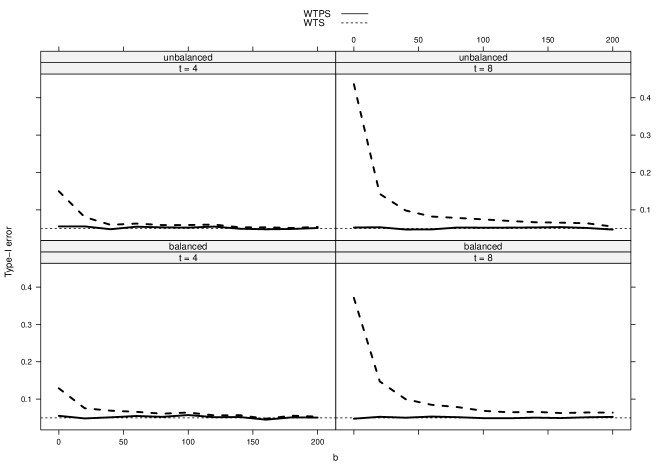
Figure 2: Type-I error rates under the interaction hypothesis for the WTS and the WTPS, where sample size was increased by adding $b{\bf 1}_{3},b=0,20,\dots,200$ to the sample size vectors in a balanced (lower panel) and unbalanced (upper panel) design with $t=4$ (left panel) and $t=8$ (right panel) time points under covariance setting 2, i.e., $\boldsymbol{V}_{i}=diag(\sigma_{1}^{2},\dots,\sigma_{t}^{2})$ with $\sigma_{s}^{2}=s$ for $t=4$ and $\sigma_{s}^{2}=\sqrt{s}$ for $t=8$.

4.3.3 Power

The power simulations are explained in detail in Section 11 of the supplementary material to this paper. Since the WTS turned out to test on different $\alpha-$levels (see the simulation results under the null hypothesis), we have excluded it from the analyses. We additionally considered the approximation described by Lecoutre (1991) as well as Hotelling’s $T^{2}$ (Hotelling, 1931). It turns out that the ATS has the highest power for normally distributed data, performing slightly better than the WTPS. For log-normally distributed data, the WTPS has larger power than the other methods and it is the only method controlling the type-I error correctly.

5 Application: Analysis of the Data Example

Finally, we analyze the data example on oxygen consumption of leukocytes in the presence and absence of inactivated staphylococci. In this setting we wish to analyze the effect of the whole-plot factor ’treatment’ (factor A, Placebo/Verum, $a=2$) as well as the sub-plot factors ’staphylococci’ (factor B, with/without, $b=2$) and ’time’ (factor T, 6/12/18 min, $t=t_{i}=3,i=1,\dots,ab$). We are also interested in interactions between the different factors. The mean values of the data are given in Table 1 in Section 1.

In the analysis we compared the three tests discussed above: The ATS in (2.4) is compared to the corresponding $F(\hat{\nu},\infty)$-quantile, the WTS in (2.5) to the asymptotic $\chi^{2}_{f}$-quantile as well as the quantile obtained by the permutation procedure (WTPS). The seven different null hypotheses of interest about main and interaction effects can be tested by choosing the related hypotheses matrices. Here, we have chosen $\boldsymbol{H}_{A}=\boldsymbol{P}_{a}\otimes\frac{1}{b}\boldsymbol{1}_{b}^{\prime}\otimes\frac{1}{t}\boldsymbol{1}_{t}^{\prime}$, $\boldsymbol{H}_{B}=\frac{1}{a}\boldsymbol{1}_{a}^{\prime}\otimes\boldsymbol{P}_{b}\otimes\frac{1}{t}\boldsymbol{1}_{t}^{\prime}$ and $\boldsymbol{H}_{T}=\frac{1}{a}\boldsymbol{1}_{a}^{\prime}\otimes\frac{1}{b}\boldsymbol{1}_{b}^{\prime}\otimes\boldsymbol{P}_{t}$ for testing the main effect of the three factors $A,B,$ and $T$. For the interaction terms we used the matrices $\boldsymbol{H}_{AT}=\boldsymbol{P}_{a}\otimes\frac{1}{b}\boldsymbol{1}_{b}^{\prime}\otimes\boldsymbol{P}_{t}$, $\boldsymbol{H}_{AB}=\boldsymbol{P}_{a}\otimes\boldsymbol{P}_{b}\otimes\frac{1}{t}\boldsymbol{1}_{t}^{\prime}$ and $\boldsymbol{H}_{BT}=\frac{1}{a}\boldsymbol{1}_{a}^{\prime}\otimes\boldsymbol{P}_{b}\otimes\boldsymbol{P}_{t},$ and $\boldsymbol{H}_{ABT}=\boldsymbol{P}_{a}\otimes\boldsymbol{P}_{b}\otimes\boldsymbol{P}_{t}$. The resulting p-values of the analysis are presented in Table 14.

Table 5: Results of the analysis of the $O_{2}$ consumption data.

	ATS	WTS	WTPS
A	0.001	0.001	$<$0.001
B	$<$0.001	$<$0.001	$<$0.001
T	$<$0.001	$<$0.001	$<$0.001
AB	0.110	0.110	0.118
AT	0.009	$<$0.001	0.001
BT	0.094	0.115	0.141
ABT	0.117	0.116	0.156

For this example all tests under considerations lead to similar conclusions: Each factor (treatment, staphylococci and time) has a significant influence on the $O_{2}$ consumption of the leukocytes. Moreover, there is a significant interaction between treatment and time.

6 Conclusions and Discussion

In this paper, we have generalized the permutation idea of Pauly et al. (2015a) for independent univariate factorial designs to the case of repeated measures allowing for a factorial structure. Here, the suggested permutation test is asymptotically valid and does not require the assumptions of multivariate normality, equal covariance matrices or balanced designs. It is based on the well-known Wald-type statistic (WTS) which possesses the beneficial property of an asymptotic pivot while being applicable for general repeated measures designs. Since it is well known for being very liberal for small and moderate sample sizes, we have considerably improved its small sample behavior under the null hypothesis by a studentized permutation technique. For univariate and independent observations the idea of this technique dates back to Neuhaus (1993) and Janssen (1997) and has recently been considered for more complex designs in independent observations by Chung and Romano (2013) and Pauly et al. (2015a).

In addition, we have rigorously proven in Theorem 3.1 that the permutation distribution of the WTS always approximates the null distribution of the WTS and can thus be applied for calculating data-dependent critical values. In particular, the result implies that the corresponding Wald-type permutation test is asymptotically exact under the null hypothesis and consistent for fixed alternatives while providing the same local power as the WTS under contiguous alternatives.

Moreover, our simulation study indicated that the permutation procedure showed a very accurate performance in all designs under consideration with moderate repeated measures (t=4) and homoscedastic or slightly heteroscedastic covariances. Only in the case of a larger number of repeated measurements (t=8) the WTPS showed a more or less liberal (conservative) behavior when testing the interaction hypothesis in an unbalanced design. However, all other competing procedures considered in the paper and the supplementary material did not perform better in these situations.

Roughly speaking, the good performance of the WTPS for finite samples may be explained by a better approximation of the underlying distribution of the WTS by the permutation distribution as compared to the $\chi^{2}$-distribution. This could be seen clearly in the distances between the quantile functions.

^∗ University of Ulm, Institute of Statistics, Germany
  email: markus.pauly@uni-ulm.de

^∗∗ University Medical Center Göttingen, Institute of Medical Statistics, Germany

8 Proofs

Proof of Theorem 2.1: First note that $\boldsymbol{T}=\boldsymbol{T}^{\prime}$ as well as $\boldsymbol{T}^{2}=\boldsymbol{T}$. Let $\boldsymbol{T}\boldsymbol{\mu}=\frac{\boldsymbol{T}\boldsymbol{\nu}}{\sqrt{N}}$ for $\boldsymbol{\nu}\in\mathbb{R}^{T}$, i.e., for $\boldsymbol{\nu}={\bf 0}$ we are working under $H_{0}$. It holds that $\sqrt{N}(\boldsymbol{\overline{Y}}_{\cdot}-\boldsymbol{\mu})$ has, asymptotically, a multivariate normal distribution with mean $\boldsymbol{\nu}$ and covariance matrix $\boldsymbol{\Sigma}$. Thus, it follows that

$$N\boldsymbol{\overline{Y}}_{\cdot}^{\prime}\boldsymbol{T}\boldsymbol{\overline{Y}}_{\cdot}\to\boldsymbol{Z}^{\prime}\boldsymbol{T}\boldsymbol{Z},$$

with $\boldsymbol{Z}\sim N(\boldsymbol{\nu},\boldsymbol{\Sigma})$. If additionally $\boldsymbol{\Sigma}>0$, we may write $\boldsymbol{Z}=\boldsymbol{\Sigma}^{1/2}\tilde{\boldsymbol{Z}}$ where $\tilde{\boldsymbol{Z}}\sim N(\boldsymbol{\Sigma}^{-1/2}\boldsymbol{\nu},\boldsymbol{I})$ and thus $\boldsymbol{Z}^{\prime}\boldsymbol{T}\boldsymbol{Z}=\sum_{i=1}^{a}\sum_{s=1}^{t_{i}}\lambda_{is}X_{is}$ where $\lambda_{is}$ are the eigenvalues of $\boldsymbol{T}\boldsymbol{\Sigma}$ and $X_{is}\sim\chi^{2}_{1}(\delta)$ for $\delta=\boldsymbol{\nu}^{\prime}\boldsymbol{\Sigma}^{-1}\boldsymbol{\nu}$. $\Box$

Proof of Theorem 2.2: The null distribution of the WTS follows analogous to the proof of Theorem 2.1 in Konietschke et al. (2015). Obviously, $\varphi_{WTS}$ is an asymptotic level $\alpha$ test and consistent for fixed alternatives $\boldsymbol{H}\boldsymbol{\mu}\neq{\bf 0}$.
Under $H_{1}:\boldsymbol{H}\boldsymbol{\mu}=\frac{1}{\sqrt{N}}\boldsymbol{\nu}$, it holds that $\sqrt{N}\boldsymbol{H}\boldsymbol{\overline{Y}}_{\cdot}$ has, asymptotically, an $N(\boldsymbol{H}\boldsymbol{\nu},\boldsymbol{H}\boldsymbol{\Sigma}\boldsymbol{H}^{\prime})$ distribution. Thus, the WTS has asymptotically a non-central $\chi^{2}_{f}(\tilde{\delta})$ distribution with $f=rank(\boldsymbol{H})$ degrees of freedom and non-centrality parameter $\tilde{\delta}=(\boldsymbol{H}\boldsymbol{\nu})^{\prime}(\boldsymbol{H}\boldsymbol{\Sigma}\boldsymbol{H}^{\prime})^{+}\boldsymbol{H}\boldsymbol{\nu}$. $\Box$

We will now proof Theorem 3.1. For notational convenience, we introduce

$$\boldsymbol{Z}=(Z_{N,1},\dots,Z_{N,\tilde{N}})=(Y_{111},Y_{121},\dots,Y_{1n_{1}1},Y_{112},\dots,Y_{an_{a}t_{a}})$$

for the pooled sample. Since $\boldsymbol{H}\boldsymbol{1}=\boldsymbol{0}$ we can rewrite the permuted test statistic as

$$Q_{N}^{\pi}=\sqrt{N}(\boldsymbol{\overline{Y}}_{\cdot}^{\pi}-\boldsymbol{\overline{Y}}_{\ldots})^{\prime}\boldsymbol{H}^{\prime}(\boldsymbol{H}\boldsymbol{\widehat{\Sigma}}^{\pi}\boldsymbol{H}^{\prime})^{+}\sqrt{N}\boldsymbol{H}(\boldsymbol{\overline{Y}}_{\cdot}^{\pi}-\boldsymbol{\overline{Y}}_{\ldots}),$$

where $\boldsymbol{\overline{Y}}_{\ldots}=\overline{Y}_{\ldots}\cdot\boldsymbol{1}_{T}$ and $\overline{Z}_{\tilde{N}}=\overline{Y}_{\ldots}=\frac{1}{\tilde{N}}\sum_{i=1}^{\tilde{N}}{Z_{N,i}}$. Based on this representation, we can split the proof of Theorem 3.1 in two results. There, we first show that the conditional distribution of $\sqrt{N}(\boldsymbol{\overline{Y}}_{\cdot}^{\pi}-\boldsymbol{\overline{Y}}_{\ldots})$ given the data is asymptotically multivariate normal. However, it turns out that the resulting covariance matrix is different from $\boldsymbol{\Sigma}$. Our approach corrects for the ’wrong’ covariance structure by studentizing with $\boldsymbol{\widehat{\Sigma}}^{\pi}$, which is shown in a second step. Altogether, this proves the consistency of the WTPS as stated in Theorem 3.1 as well as the properties of the corresponding test mentioned in Remarks 3.1 and 3.2.

Note that there exist finite limits $b_{i}=\lim_{\min(n_{i})\to\infty}\frac{\tilde{N}}{n_{i}}\in(1,\infty),i=1,\dots,a$ because of (1) and $0<\max_{i=1,\dots,a}(t_{i})<\infty$.

Lemma 8.1

Under the assumptions of Theorem 3.1, the conditional permutation distribution of

$$\sqrt{N}(\boldsymbol{\overline{Y}}_{\cdot}^{\pi}-\boldsymbol{\overline{Y}}_{\ldots})$$

given the observed data $\boldsymbol{Y}$ weakly converges to a multivariate normal — $N({\bf 0},\sigma^{2}\boldsymbol{\Gamma})$ — distribution in probability, where

$$\sigma^{2}=\sum_{i=1}^{a}\frac{1}{b_{i}}\sum_{s=1}^{t_{i}}(\sigma^{2}_{is}+\mu^{2}_{is})-\left(\sum_{i=1}^{a}\frac{1}{b_{i}}\sum_{s=1}^{t_{i}}\mu_{is}\right)^{2}$$ (8.1)

with $\sigma_{is}^{2}=\operatorname{{\it Var}}(Y_{iks})$ and

$$\boldsymbol{\Gamma}=\bigoplus_{i=1}^{a}\kappa_{i}^{-1}\boldsymbol{I}_{t_{i}}-\boldsymbol{J}_{T}=\operatorname{\it diag}(\kappa_{1}^{-1}\boldsymbol{I}_{t_{1}},\dots,\kappa_{a}^{-1}\boldsymbol{I}_{t_{a}})-\boldsymbol{J}_{T}.$$ (8.2)

Proof: First note that the classical Cramér-Wold device cannot be applied directly in this context due to the occurrence of uncountably many exceptional sets. Therefore we will apply a modified Cramér-Wold device, see e.g. the proof of Theorem 4.1 in Pauly (2011). Let $D$ be a dense and countable subset of $\mathbb{R}^{T}$. Then for every fixed $\mbox{\boldmath$\lambda$}=(\lambda_{1},\dots,\lambda_{T})\in D$ and $M_{0}=0,M_{1}=n_{1},\dots,M_{t_{1}}=t_{1}n_{1},M_{t_{1}+1}=t_{1}n_{1}+n_{2},\dots,M_{T}=\tilde{N}$, we have

$$\sqrt{N}\mbox{\boldmath$\lambda$}^{\prime}\boldsymbol{\overline{Y}}_{\cdot} = \sum_{i=1}^{a}\sum_{k=M_{i-1}+1}^{M_{i}}\frac{\sqrt{N}}{n_{i}}\lambda_{i}Z_{N,k}$$

$$= \sqrt{N}\sum_{s=1}^{\tilde{N}}c_{Ns}\frac{Z_{N,s}}{\sqrt{\tilde{N}}},$$

where $c_{Ns}=\sqrt{\tilde{N}}\sum_{i=1}^{T}{\mathds{1}}\{M_{i-1}+1\leq s\leq M_{i}\}\frac{\lambda_{i}}{n_{i}}$. This implies

$$\sqrt{N}\boldsymbol{\lambda}^{\prime}(\boldsymbol{\overline{Y}}_{\cdot}^{\pi}-\boldsymbol{\overline{Y}}_{\ldots}) = \sqrt{N}\sum_{s=1}^{\tilde{N}}c_{Ns}\frac{(Z_{N,\pi(s)}-\overline{Z}_{\tilde{N}})}{\sqrt{\tilde{N}}}$$

$$\stackrel{{\scriptstyle d}}{{=}} \sqrt{N}\sum_{s=1}^{\tilde{N}}c_{N\pi(s)}\frac{Z_{N,s}-\overline{Z}_{\tilde{N}}}{\sqrt{\tilde{N}}},$$

since $\pi$ is uniformly distributed on the set of all permutations of the numbers $\{1,\dots,\tilde{N}\}$. Let $b_{i}=\lim_{\min(n_{i})\to\infty}\frac{\tilde{N}}{n_{i}}$ with $b_{i}<\infty$ because of (1) and $\max(t_{i})<\infty$.

We now apply Theorem 4.1 in Pauly (2011) to prove the conditional convergence in distribution. Therefore, we have to prove the following conditions:

$$\frac{1}{\sqrt{\tilde{N}}}\max_{1\leq i\leq\tilde{N}}|Z_{N,i}-\overline{Z}_{\tilde{N}}| \stackrel{{\scriptstyle P}}{{\to}} 0$$ (8.4)

$$\frac{1}{\tilde{N}}\sum_{i=1}^{\tilde{N}}(Z_{N,i}-\overline{Z}_{\tilde{N}})^{2} \stackrel{{\scriptstyle P}}{{\to}} \sigma^{2}$$ (8.5)

$$\max_{1\leq s\leq\tilde{N}}|c_{N,s}-\overline{c}_{\cdot}| \stackrel{{\scriptstyle P}}{{\to}} 0$$ (8.6)

$$\sum_{s=1}^{\tilde{N}}(c_{N,s}-\overline{c}_{\cdot})^{2} \stackrel{{\scriptstyle P}}{{\to}} \sigma^{2}_{\lambda}=\sum_{i=1}^{T}\lambda_{i}^{2}b_{i}-\left(\sum_{i=1}^{T}\lambda_{i}\right)^{2}$$ (8.7)

$$\sqrt{\tilde{N}}(c_{N,\pi(1)}-\overline{c}_{\cdot}) \stackrel{{\scriptstyle d}}{{\to}} W\text{ with }E(W)=0\text{ and }\operatorname{{\it Var}}(W)=\sigma_{\lambda}^{2}$$ (8.8)

Condition (8.4) as well as (8.6) – (8.8) follow analogous to Pauly et al. (2015a): Since the random variables within each of the $a$ groups are i.i.d. with finite variance, they fulfill (8.4). The convergence in (8.6) is obvious and since $\sqrt{\tilde{N}}\cdot\overline{c}_{\cdot}=\sum_{i=1}^{T}\lambda_{i}$ we have

$$\sum_{s=1}^{\tilde{N}}(c_{N,s}-\overline{c}_{\cdot})^{2} = \sum_{s=1}^{\tilde{N}}c_{N,s}^{2}-(\sqrt{\tilde{N}}\overline{c}_{\cdot})^{2}=\sum_{i=1}^{T}\frac{\tilde{N}}{n_{i}}\lambda_{i}^{2}-\left(\sum_{i=1}^{T}\lambda_{i}\right)^{2}$$

$$\stackrel{{\scriptstyle P}}{{\to}} \sum_{i=1}^{T}\lambda_{i}^{2}b_{i}-\left(\sum_{i=1}^{T}\lambda_{i}\right)^{2}=\sigma_{\lambda}^{2}.$$

Moreover, (8.8) holds due to

$$P\left(\sqrt{\tilde{N}}c_{N,\pi(1)}=\frac{\tilde{N}\lambda_{i}}{n_{i}}\right)=\frac{n_{i}}{\tilde{N}}\to\frac{1}{b_{i}}$$

for $1\leq i\leq a$, i.e., for a random variable $\widetilde{W}$ with $P(\widetilde{W}=b_{i}\lambda_{i})=\frac{1}{b_{i}}$, $1\leq i\leq a$, we have

$$\sqrt{\tilde{N}}(c_{N,\pi(1)}-\overline{c}_{\cdot})\stackrel{{\scriptstyle d}}{{\to}}\widetilde{W}-\sum_{i=1}^{T}\lambda_{i}=W,$$

where $W$ fulfills $E(W)=0$ and $\operatorname{{\it Var}}(W)=\sigma_{\lambda}^{2}$. It remains to prove (8.5):

$$\frac{1}{\tilde{N}}\sum_{i=1}^{\tilde{N}}(Z_{N,i}-\overline{Z}_{\tilde{N}})^{2}=\frac{1}{\tilde{N}}\sum_{i=1}^{\tilde{N}}Z_{N,i}^{2}-\overline{Y}_{\ldots}^{2}.$$

Consider

$$E\left(\frac{1}{\tilde{N}}\sum_{i=1}^{\tilde{N}}Z_{N,i}^{2}\right) = \frac{1}{\tilde{N}}\sum_{i=1}^{a}\sum_{s=1}^{t_{i}}\sum_{k=1}^{n_{i}}E\left(Y_{iks}^{2}\right)$$

$$= \frac{1}{\tilde{N}}\sum_{i=1}^{a}\sum_{s=1}^{t_{i}}\sum_{k=1}^{n_{i}}(\sigma_{is}^{2}+\mu_{is}^{2})$$

$$= \sum_{i=1}^{a}\frac{n_{i}}{\tilde{N}}\sum_{s=1}^{t_{i}}(\sigma_{is}^{2}+\mu_{is}^{2})$$

$$\to \sum_{i=1}^{a}\frac{1}{b_{i}}\sum_{s=1}^{t_{i}}(\sigma_{is}^{2}+\mu_{is}^{2}).$$

Furthermore:

$$E(\overline{Y}_{\ldots}^{2}) = E\left(\left(\frac{1}{\tilde{N}}\sum_{i=1}^{\tilde{N}}Z_{N,i}\right)^{2}\right)$$

$$= \underbrace{\operatorname{{\it Var}}\left(\frac{1}{\tilde{N}}\sum_{i=1}^{a}\sum_{s=1}^{t_{i}}\sum_{k=1}^{n_{i}}Y_{iks}\right)}_{{\mathcal{O}}(\frac{1}{N})}+\left(E\left(\frac{1}{\tilde{N}}\sum_{i=1}^{a}\sum_{s=1}^{t_{i}}\sum_{k=1}^{n_{i}}Y_{iks}\right)\right)^{2}$$

$$\to \left(\sum_{i=1}^{a}\frac{1}{b_{i}}\sum_{s=1}^{t_{i}}\mu_{is}\right)^{2}$$

Since

$$\operatorname{{\it Var}}\left(\frac{1}{\tilde{N}}\sum_{i=1}^{\tilde{N}}(Z_{N,i}-\overline{Z}_{\tilde{N}})^{2}\right) = \operatorname{{\it Var}}\left(\sum_{i=1}^{a}\frac{1}{\tilde{N}}\sum_{s=1}^{t_{i}}\sum_{k=1}^{n_{i}}Y_{iks}^{2}-\overline{Y}_{\ldots}^{2}\right)$$

$$= \sum_{i=1}^{a}\frac{1}{(\tilde{N})^{2}}\sum_{k=1}^{n_{i}}\operatorname{{\it Var}}\left(\sum_{s=1}^{t_{i}}(Y_{iks}^{2}-\frac{1}{\tilde{N}}\overline{Y}_{\ldots}^{2})\right)$$

$$= {\mathcal{O}}\left(\frac{1}{N}\right)$$

because of independence and condition (2), the desired conclusion follows with Tschebyscheff’s inequality.

Altogether, this implies by Theorem 4.1 in Pauly (2011) convergence in distribution given the data $\boldsymbol{Y}$

$$\sqrt{N}\boldsymbol{\lambda}^{\prime}(\boldsymbol{\overline{Y}}_{\cdot}^{\pi}-\boldsymbol{\overline{Y}}_{\ldots})\stackrel{{\scriptstyle d}}{{\to}}N(0,\sigma^{2}\sigma_{\lambda}^{2})$$ (8.10)

in probability. This convergence holds for every fixed $\mbox{\boldmath$\lambda$}\in D$. Applying the subsequential principle for convergence in probability we can find a common subsequence such that (8.10) holds almost surely for all $\mbox{\boldmath$\lambda$}\in D$ along this subsequence. Now continuity of the characteristic function of the limit and tightness of the conditional distribution of $\sqrt{N}(\boldsymbol{\overline{Y}}_{\cdot}^{\pi}-\boldsymbol{\overline{Y}}_{\ldots})$ given $\boldsymbol{Y}$ show that (8.10) holds almost surely for all $\mbox{\boldmath$\lambda$}\in\mathbb{R}^{T}$ along this subsequence. Thus, an application of the classical Cramér-Wold device together with another application of the subsequence principle imply the result. $\Box$

Now we will study the convergence of $\boldsymbol{\widehat{\Sigma}}^{\pi}=N\boldsymbol{\widehat{V}}^{\pi}=\bigoplus_{i=1}^{a}\frac{N}{n_{i}}\boldsymbol{\widehat{V}}_{i}^{\pi}$.

Lemma 8.2

Under the assumptions of Theorem 3.1 we have convergence in probability

$$\boldsymbol{\widehat{\Sigma}}^{\pi}\stackrel{{\scriptstyle P}}{{\to}}\sigma^{2}\operatorname{\it diag}(\kappa_{1}^{-1}\boldsymbol{I}_{t_{i}},\dots,\kappa_{a}^{-1}\boldsymbol{I}_{t_{a}})$$

as $N\to\infty$.

Proof: It suffices to show that $(\boldsymbol{\widehat{V}}_{i}^{\pi})_{r,s}\stackrel{{\scriptstyle P}}{{\to}}\sigma^{2}{\mathds{1}}\{r=s\}$ in probability for all $1\leq r,s\leq t_{i}$. Therefore consider

$$\frac{n_{i}-1}{n_{i}}(\boldsymbol{\widehat{V}}_{i}^{\pi})_{r,s}=\underbrace{\frac{1}{n_{i}}\sum_{k=1}^{n_{i}}Y_{ikr}^{\pi}Y_{iks}^{\pi}}_{A}-\underbrace{\overline{Y}_{i\cdot r}^{\pi}\overline{Y}_{i\cdot s}^{\pi}}_{B}$$

First, consider $B$. It holds:

$$E(\overline{Y}_{i\cdot r}^{\pi}|\boldsymbol{Y})\stackrel{{\scriptstyle P}}{{\to}}\sum_{i=1}^{a}\frac{1}{b_{i}}\sum_{s=1}^{t_{i}}\mu_{is}$$

for all $r$ and all $i$ analogous to (8). Furthermore, setting $d_{N,s}^{(i)}:={\mathds{1}}\{(r-1)n_{i}+1\leq s\leq rn_{i}\}/n_{i}$ for $1\leq s\leq\tilde{N}$ and using Theorem 3 from Hájek et al. (1999) we get convergence in probability of the corresponding conditional variance

$$\operatorname{{\it Var}}\left(\overline{Y}_{i\cdot r}^{\pi}|\boldsymbol{Y}\right) = \operatorname{{\it Var}}\left(\sum_{s=1}^{\tilde{N}}d_{N,s}^{(i)}Z_{N,\pi(s)}|\boldsymbol{Z}\right)$$

$$= \sum_{s=1}^{\tilde{N}}\left(d_{N,s}^{(i)}-\overline{d}_{N,\cdot}^{(i)}\right)^{2}\frac{1}{\tilde{N}-1}\sum_{s=1}^{\tilde{N}}(Z_{N,s}-\overline{Z}_{\tilde{N}})^{2}\stackrel{{\scriptstyle P}}{{\to}}0,$$

since $\sum_{s=1}^{\tilde{N}}\left(d_{N,s}^{(i)}-\overline{d}_{N,\cdot}^{(i)}\right)^{2}\to 0$ as $N\to\infty$ and $\frac{1}{\tilde{N}-1}\sum_{s=1}^{\tilde{N}}(Z_{N,s}-\overline{Z}_{\tilde{N}})^{2}=\mathcal{O}_{P}(1)$. Altogether this implies convergence in probability by the continuous mapping theorem

$$B\stackrel{{\scriptstyle P}}{{\to}}\left(\sum_{i=1}^{a}\frac{1}{b_{i}}\sum_{s=1}^{t_{i}}\mu_{is}\right)^{2}.$$

For part $A$ we distinguish two cases: First, assume $r=s$. We have

$$A=\frac{1}{n_{i}}\sum_{k=(r-1)n_{i}+1}^{rn_{i}}Z_{N,\pi(k)}^{2}.$$

Now consider the conditional expectation of $A$

$$E(A|\boldsymbol{Y}) = \frac{1}{\tilde{N}}\sum_{i=1}^{a}\sum_{r=1}^{t_{i}}\frac{1}{n_{i}}\sum_{k=(r-1)n_{i}+1}^{rn_{i}}Z_{N,k}^{2}$$

$$\stackrel{{\scriptstyle P}}{{\to}} \sum_{i=1}^{a}\frac{1}{b_{i}}\sum_{s=1}^{t_{i}}(\sigma_{is}^{2}+\mu_{is}^{2})$$

as well as

$$\operatorname{{\it Var}}(A|\boldsymbol{Y}) = \operatorname{{\it Var}}\left(\sum_{s=1}^{\tilde{N}}d_{N,s}^{(i)}Z_{N,\pi(s)}^{2}|\boldsymbol{Z}\right)$$

$$= \sum_{s=1}^{\tilde{N}}\left(d_{N,s}^{(i)}-d_{N,\cdot}^{-(i)}\right)^{2}\frac{1}{\tilde{N}-1}\sum_{s=1}^{\tilde{N}}\left(Z_{N,s}^{2}-\frac{1}{\tilde{N}-1}\sum_{r=1}^{\tilde{N}}Z_{N,r}^{2}\right)^{2},$$

which converges to 0 in probability as above and since we have
$\frac{1}{\tilde{N}-1}\sum_{s=1}^{\tilde{N}}\left(Z_{N,s}^{2}-\frac{1}{\tilde{N}-1}\sum_{r=1}^{\tilde{N}}Z_{N,r}^{2}\right)^{2}=\mathcal{O}_{P}(1)$ because of the existence of fourth moments.

Now, consider $r\neq s$. We have that

$$E(A|\boldsymbol{Y}) = \frac{1}{n_{i}}\sum_{k=1}^{n_{i}}E(Y_{ikr}^{\pi}Y_{iks}^{\pi}|\boldsymbol{Y})=E(Y_{111}^{\pi}Y_{112}^{\pi}|\boldsymbol{Y}){\color[rgb]{1,0,0}?}$$

$$= \frac{1}{(\tilde{N})!}\sum_{\pi\in\mathcal{S}_{\tilde{N}}}Z_{N,\pi(1)}Z_{N,\pi(2)}$$

$$= \frac{1}{\tilde{N}(\tilde{N}-1)}\sum_{i\neq j}Z_{N,i}Z_{N,j}$$

Consider $E(Z_{N,i}Z_{N,j})$. There are two possibilities: If $Z_{N,i}$ and $Z_{N,j}$ stem from different random vectors (i.e., from different individuals) they are independent and we can write $E(Z_{N,i}Z_{N,j})=E(Z_{N,i})E(Z_{N,j})$. If they stem from the same individual, we cannot rewrite the expectation and we denote it by $\gamma_{i,j}:=E(Z_{N,i}Z_{N,j})\in(-\infty,\infty)$. For every fixed $i$ there are $(t_{i}-1)$ possible $j$’s such that $Z_{N,i}$ and $Z_{N,j}$ come from the same individual. This implies:

$$E\left(\frac{1}{\tilde{N}(\tilde{N}-1)}\sum_{i\neq j}Z_{N,i}Z_{N,j}\right) = \frac{1}{\tilde{N}(\tilde{N}-1)}\sum_{(i,j)\in\Xi}E(Z_{N,i})E(Z_{N,j})$$

$$+ \frac{1}{\tilde{N}(\tilde{N}-1)}\sum_{i=1}^{\tilde{N}}\sum_{(i,j)\in\varLambda}\gamma_{i,j},$$

where the index sets are defined as $\Xi=\{(i,j,):i\neq j\text{ and }i,j\text{ stem from different subjects}\}$ and $\varLambda=\{(i,j):i\neq j\text{ and }i,j\text{ stem from the same subject}\}$.
Because of the Cauchy-Schwarz inequality and Condition (2) it holds that

$$\sup_{i,j}|\gamma_{i,j}|\leq 2\sup_{i}E(Z_{N,i}^{2})\leq C<\infty.$$

Thus, it follows that

$$\frac{1}{\tilde{N}(\tilde{N}-1)}\sum_{i=1}^{\tilde{N}}\sum_{(i,j)\in\varLambda}\gamma_{i,j}\leq\frac{\tilde{N}(\max{t_{i}}-1)}{\tilde{N}(\tilde{N}-1)}C\to 0$$

as $N\to\infty$. For the first summand on the right hand side in Equation (8), it holds that

$$\frac{1}{\tilde{N}(\tilde{N}-1)}\sum_{(i,j)\in\Xi}E(Z_{N,i})E(Z_{N,j}) = \frac{1}{\tilde{N}(\tilde{N}-1)}\sum_{i=1}^{a}\sum_{s=1}^{t_{i}}\sum_{j=1}^{a}\sum_{r=1}^{t_{j}}\mu_{is}\mu_{jr}-o(1)$$

$$\to \left(\sum_{i=1}^{a}\frac{1}{b_{i}}\sum_{s=1}^{t_{i}}\mu_{is}\right)^{2}.$$

To complete the proof it remains to show that $\operatorname{{\it Var}}\left(\frac{1}{\tilde{N}(\tilde{N}-1)}\sum_{i\neq j}Z_{N,i}Z_{N,j}\right)\to 0$. Thus,

$$\operatorname{{\it Var}}\left(\frac{1}{\tilde{N}(\tilde{N}-1)}\sum_{i\neq j}Z_{N,i}Z_{N,j}\right) = \frac{1}{(\tilde{N}(\tilde{N}-1))^{2}}\sum_{i_{1}\neq j_{1}}\sum_{i_{2}\neq j_{2}}\operatorname{{\it Cov}}(Z_{N,i_{1}}Z_{N,j_{1}},Z_{N,i_{2}}Z_{N,j_{2}}).$$

As above, we distinguish between the cases $(i,j)\in\Xi$ and $(i,j)\in\varLambda$. If $Z_{N,i_{1}}Z_{N,j_{1}}$ and $Z_{N,i_{2}}Z_{N,j_{2}}$ stem from different individuals it holds that $\operatorname{{\it Cov}}(Z_{N,i_{1}}Z_{N,j_{1}},Z_{N,i_{2}}Z_{N,j_{2}})=0$ because of independence. In all other cases it holds that

$$\operatorname{{\it Cov}}(Z_{N,i_{1}}Z_{N,j_{1}},Z_{N,i_{2}}Z_{N,j_{2}})\leq 2\sup_{i}E(Z_{N,i}^{4})=\tilde{C}<\infty$$

because of assumption (2) and the Cauchy-Schwarz inequality.
Furthermore, for every fixed $i_{1}$ and $j_{1}$ there are less than $5(\max{t_{i}})^{4}$ possibilities for $Z_{N,i_{2}}Z_{N,j_{2}}$ to stem from the same individual(s) as $Z_{N,i_{1}}Z_{N,j_{1}}$, such that at least one of the sums cancels out and $\operatorname{{\it Var}}\left(\frac{1}{\tilde{N}(\tilde{N}-1)}\sum_{i\neq j}Z_{N,i}Z_{N,j}\right)\to 0$ for all $i,j$ as $N\to\infty$.

This implies that for $r\neq s$

$$\frac{n_{i}-1}{n_{i}}\left(\boldsymbol{\widehat{V}}_{i}^{\pi}\right)_{r,s}=A-B\stackrel{{\scriptstyle P}}{{\to}}\left(\sum_{i=1}^{a}\frac{1}{b_{i}}\sum_{s=1}^{t_{i}}\mu_{is}\right)^{2}-\left(\sum_{i=1}^{a}\frac{1}{b_{i}}\sum_{s=1}^{t_{i}}\mu_{is}\right)^{2}=0$$

and for $r=s$ we have $(\boldsymbol{\widehat{V}}_{i}^{\pi})_{r,s}\stackrel{{\scriptstyle P}}{{\to}}\sigma^{2}$. Altogether, this proves the desired result. $\Box$

We are now able to prove Theorem 3.1.
Proof: Applying the continuous mapping theorem together with Lemma 8.1 yields conditional convergence in distribution given $\boldsymbol{Y}$

$$\boldsymbol{H}\sqrt{N}(\boldsymbol{\overline{Y}}_{\cdot}^{\pi}-\boldsymbol{\overline{Y}}_{\ldots})\stackrel{{\scriptstyle d}}{{\to}}N(0,\sigma^{2}\boldsymbol{H}\boldsymbol{D}\boldsymbol{H}^{\prime}),$$

where $\boldsymbol{D}:=\operatorname{\it diag}(\kappa_{1}^{-1}\boldsymbol{I}_{t_{1}},\dots,\kappa_{a}^{-1}\boldsymbol{I}_{t_{a}})$. Moreover, we have convergence in probability

$$\boldsymbol{H}\boldsymbol{\widehat{\Sigma}}^{\pi}\boldsymbol{H}^{\prime}\stackrel{{\scriptstyle P}}{{\to}}\sigma^{2}\boldsymbol{H}\boldsymbol{D}\boldsymbol{H}^{\prime}$$

by Lemma 8.2. Since $\det(\boldsymbol{\widehat{V}}_{i}^{\pi})>0$ almost surely for $N$ large enough due to $\boldsymbol{\Sigma}>0$, the corresponding Moore-Penrose inverse converges as well in probability and hence another application of the continuous mapping theorem proves the result using Theorem 9.2.2 in Rao and Mitra (1971). $\Box$

9 Other resampling approaches

9.1 Nonparametric bootstrap approach

Here, we consider a nonparametric bootstrap sample $\boldsymbol{Y}^{*}=(Y_{111}^{*},\ldots,Y_{an_{a}t}^{*})$ drawn with replacement from the pooled observation vector $\boldsymbol{Y}=(Y_{111},\ldots,Y_{an_{a}t})$. Therefore, given the observations, the bootstrap components are all independent with identical distribution which is given by the empirical distribution of $\boldsymbol{Y}^{*}$. The WTS of the bootstrap sample is given by

$$Q_{N}^{*}=N(\boldsymbol{\overline{Y}}_{\cdot}^{*})^{\prime}\boldsymbol{H}^{\prime}(\boldsymbol{H}\boldsymbol{\widehat{\Sigma}}^{*}\boldsymbol{H}^{\prime})^{+}\boldsymbol{H}\boldsymbol{\overline{Y}}_{\cdot}^{*},$$

where $\boldsymbol{\overline{Y}}_{\cdot}^{*}$ is the vector of means of the bootstrap sample and $\boldsymbol{\widehat{\Sigma}}^{*}$ denotes their covariance matrix.

Theorem 9.1

The distribution of $Q_{N}^{*}$ conditioned on the observed data $\boldsymbol{Y}$ weakly converges to the central $\chi^{2}_{f}$ distribution in probability, where $f=rank(\boldsymbol{H})$. In particular, we have

$$\sup_{x\in\mathbb{R}}\left|P_{\boldsymbol{\mu}}(Q_{N}^{*}\leq x|\boldsymbol{Y})-P_{\boldsymbol{\mu}_{0}}(Q_{N}\leq x)\right|\to 0$$ (9.1)

in probability for any underlying parameter $\boldsymbol{\mu}\in\mathbb{R}^{at}$ and $\boldsymbol{\mu}_{0}\in H_{0}(\boldsymbol{H})$.

Proof: The result follows analogously to the proof of Theorem 3.1 in the paper. $\Box$

Note, that a nonparametric bootstrap version based on drawing with replacement from the observation vectors as in Konietschke et al. (2015) performed considerably worse than the parametric bootstrap approach described below and is therefore not reported here.

In addition, we have also studied a nonparametric bootstrap version of the ATS (although this is in general not asymptotically correct) given by

$$F_{N}^{*}=\frac{N}{\operatorname{tr}(\boldsymbol{T}\boldsymbol{\widehat{\Sigma}}^{*})}(\boldsymbol{\overline{Y}}_{\cdot}^{*})^{\prime}\boldsymbol{T}\boldsymbol{\overline{Y}}_{\cdot}^{*}.$$

A corresponding permutation version of the ATS has not been considered since it is also asymptotically only an approximation.

9.2 Parametric bootstrap approach

We have also considered a parametric bootstrap approach as studied by, e.g. Konietschke et al. (2015). Here, the parametric bootstrap variables are generated as

$$\boldsymbol{Y}^{\star}_{i}\stackrel{{\scriptstyle i.i.d.}}{{\sim}}N(\textbf{0},\boldsymbol{\widehat{V}}_{i}),\hskip 5.69046pt1\leq i\leq a.$$

The idea behind this approach is to obtain a more accurate finite sample approximation by mimicking the given covariance structure of the original data. We can again compute the WTS and ATS from the parametric bootstrap vectors as

$$Q_{N}^{\star}=N(\boldsymbol{\overline{Y}}_{\cdot}^{\star})^{\prime}\boldsymbol{H}^{\prime}(\boldsymbol{H}\boldsymbol{\widehat{\Sigma}}^{\star}\boldsymbol{H}^{\prime})^{+}\boldsymbol{H}\boldsymbol{\overline{Y}}_{\cdot}^{\star},$$

and

$$F_{N}^{\star}=\frac{N}{\operatorname{tr}(\boldsymbol{T}\boldsymbol{\widehat{\Sigma}}^{\star})}(\boldsymbol{\overline{Y}}_{\cdot}^{\star})^{\prime}\boldsymbol{T}\boldsymbol{\overline{Y}}_{\cdot}^{\star},$$

where $\boldsymbol{\overline{Y}}_{\cdot}^{\star}$ is the vector of means of the parametric bootstrap sample and $\boldsymbol{\widehat{\Sigma}}^{\star}$ denotes their empirical covariance matrix.

Theorem 9.2

The distribution of $Q_{N}^{\star}$ conditioned on the observed data $\boldsymbol{Y}$ weakly converges to the central $\chi^{2}_{f}$ distribution in probability, where $f=rank(\boldsymbol{H})$. In particular, we have

$$\sup_{x\in\mathbb{R}}\left|P_{\boldsymbol{\mu}}(Q_{N}^{\star}\leq x|\boldsymbol{Y})-P_{\boldsymbol{\mu}_{0}}(Q_{N}\leq x)\right|\to 0$$ (9.2)

in probability for any underlying parameters $\boldsymbol{\mu},\boldsymbol{\mu}_{0}\in\mathbb{R}^{at}$ with $\boldsymbol{H}\boldsymbol{\mu}_{0}={\bf 0}$.
Furthermore, for the ATS of the parametric bootstrap sample it also holds that

$$\sup_{x\in\mathbb{R}}\left|P_{\boldsymbol{\mu}}(F_{N}^{\star}\leq x|\boldsymbol{Y})-P_{\boldsymbol{\mu}_{0}}(F_{N}\leq x)\right|\to 0$$ (9.3)

in probability for any underlying parameters $\boldsymbol{\mu},\boldsymbol{\mu}_{0}\in\mathbb{R}^{at}$ with $\boldsymbol{H}\boldsymbol{\mu}_{0}={\bf 0}$. Thus, the conditional distribution of $F_{N}^{\star}$ always approximates the null distribution of $F_{N}$.

Proof: The result for the WTS follows analogously to the proof of Theorem 3.2 in Konietschke et al. (2015). For the parametric bootstrap version of the ATS the result is obtained by the multivariate Lindeberg-Feller Theorem, the Continuous Mapping Theorem and another application of Slutsky’s Theorem. The details are left to the reader. $\Box$

9.3 Type-I error rates

In the following, we present the results of the detailed simulation studies conducted as described in Section 4 of the paper. For comparison, the results of the permutation approach are also included. The results for the hypothesis of no time effect $T$ are presented in Tables 6, 7 and 8 for the normal, log-normal and exponential distribution, respectively. The results for the hypothesis of no group $\times$ time interaction are in Tables 9, 10 and 11, respectively. The parametric bootstrap approach is denoted by PBS, the nonparametric bootstrap by NPBS. The results are again compared to the asymptotic quantiles, i.e. the $F(\hat{\nu},\infty)$-quantile for the ATS and the $\chi^{2}_{f}$-quantile for the WTS. A permutation version of the ATS has not been considered for the reasons stated above. The covariance settings and the number of simulated individuals are the same as described in Section 4.

Table 6: Simulation results for the hypothesis of no time effect with normal distribution.

normal distribution
T			$t=4$		$t=8$
Cov. Setting	$\boldsymbol{n}$	Method	ATS	WTS	ATS	WTS
1	$\boldsymbol{n}^{(1)}$	Permutation	NA	0.050	NA	0.050
		PBS	0.041	0.052	0.034	0.059
		NPBS	0.048	0.047	0.052	0.050
		asymptotic	0.046	0.085	0.040	0.177
	$\boldsymbol{n}^{(2)}$	Permutation	NA	0.048	NA	0.052
		PBS	0.041	0.050	0.034	0.060
		NPBS	0.046	0.048	0.052	0.050
		asymptotic	0.046	0.086	0.040	0.177
	$\boldsymbol{n}^{(3)}$	Permutation	NA	0.051	NA	0.052
		PBS	0.045	0.048	0.040	0.050
		NPBS	0.051	0.051	0.050	0.052
		asymptotic	0.050	0.078	0.043	0.135
2	$\boldsymbol{n}^{(1)}$	Permutation	NA	0.050	NA	0.051
		PBS	0.046	0.052	0.036	0.059
		NPBS	0.056	0.051	0.054	0.050
		asymptotic	0.051	0.085	0.042	0.177
	$\boldsymbol{n}^{(2)}$	Permutation	NA	0.051	NA	0.052
		PBS	0.046	0.052	0.036	0.060
		NPBS	0.057	0.051	0.056	0.052
		asymptotic	0.052	0.086	0.043	0.177
	$\boldsymbol{n}^{(3)}$	Permutation	NA	0.051	NA	0.052
		PBS	0.049	0.048	0.038	0.049
		NPBS	0.059	0.049	0.054	0.051
		asymptotic	0.053	0.077	0.041	0.135
3	$\boldsymbol{n}^{(1)}$	Permutation	NA	0.052	NA	0.062
		PBS	0.041	0.052	0.040	0.064
		NPBS	0.052	0.052	0.069	0.061
		asymptotic	0.046	0.092	0.044	0.198
	$\boldsymbol{n}^{(2)}$	Permutation	NA	0.045	NA	0.042
		PBS	0.047	0.052	0.043	0.056
		NPBS	0.056	0.043	0.075	0.042
		asymptotic	0.051	0.080	0.048	0.155
	$\boldsymbol{n}^{(3)}$	Permutation	NA	0.053	NA	0.054
		PBS	0.047	0.050	0.044	0.049
		NPBS	0.058	0.051	0.073	0.052
		asymptotic	0.051	0.078	0.048	0.136

Table 7: Simulation results for the hypothesis of no time effect with log-normal distribution.

log-normal distribution
T			$t=4$		$t=8$
Cov. Setting	$\boldsymbol{n}$	Method	ATS	WTS	ATS	WTS
1	$\boldsymbol{n}^{(1)}$	Permutation	NA	0.051	NA	0.047
		PBS	0.026	0.055	0.017	0.075
		NPBS	0.051	0.050	0.047	0.048
		asymptotic	0.032	0.094	0.021	0.198
	$\boldsymbol{n}^{(2)}$	Permutation	NA	0.052	NA	0.046
		PBS	0.025	0.058	0.016	0.074
		NPBS	0.048	0.051	0.054	0.046
		asymptotic	0.031	0.090	0.020	0.198
	$\boldsymbol{n}^{(3)}$	Permutation	NA	0.051	NA	0.048
		PBS	0.026	0.056	0.019	0.077
		NPBS	0.052	0.050	0.051	0.050
		asymptotic	0.031	0.089	0.021	0.186
2	$\boldsymbol{n}^{(1)}$	Permutation	NA	0.067	NA	0.053
		PBS	0.035	0.072	0.018	0.084
		NPBS	0.060	0.066	0.052	0.053
		asymptotic	0.040	0.110	0.022	0.207
	$\boldsymbol{n}^{(2)}$	Permutation	NA	0.067	NA	0.051
		PBS	0.034	0.073	0.018	0.082
		NPBS	0.061	0.066	0.057	0.052
		asymptotic	0.040	0.107	0.022	0.203
	$\boldsymbol{n}^{(3)}$	Permutation	NA	0.070	NA	0.057
		PBS	0.037	0.072	0.021	0.080
		NPBS	0.065	0.068	0.057	0.057
		asymptotic	0.042	0.107	0.024	0.197
3	$\boldsymbol{n}^{(1)}$	Permutation	NA	0.057	NA	0.064
		PBS	0.027	0.059	0.021	0.082
		NPBS	0.054	0.058	0.063	0.064
		asymptotic	0.033	0.101	0.024	0.221
	$\boldsymbol{n}^{(2)}$	Permutation	NA	0.053	NA	0.048
		PBS	0.031	0.060	0.028	0.075
		NPBS	0.057	0.053	0.079	0.047
		asymptotic	0.037	0.090	0.033	0.190
	$\boldsymbol{n}^{(3)}$	Permutation	NA	0.057	NA	0.062
		PBS	0.031	0.059	0.027	0.079
		NPBS	0.057	0.054	0.075	0.062
		asymptotic	0.036	0.092	0.031	0.191

Table 8: Simulation results for the hypothesis of no time effect with exponential distribution.

exponential distribution
T			$t=4$		$t=8$
Cov. Setting	$\boldsymbol{n}$	Method	ATS	WTS	ATS	WTS
1	$\boldsymbol{n}^{(1)}$	Permutation	NA	0.048	NA	0.051
		PBS	0.038	0.055	0.026	0.070
		NPBS	0.052	0.049	0.052	0.051
		asymptotic	0.045	0.090	0.034	0.194
	$\boldsymbol{n}^{(2)}$	Permutation	NA	0.053	NA	0.048
		PBS	0.039	0.057	0.029	0.069
		NPBS	0.053	0.053	0.050	0.048
		asymptotic	0.046	0.096	0.032	0.191
	$\boldsymbol{n}^{(3)}$	Permutation	NA	0.054	NA	0.050
		PBS	0.041	0.057	0.031	0.059
		NPBS	0.053	0.054	0.049	0.050
		asymptotic	0.046	0.086	0.034	0.151
2	$\boldsymbol{n}^{(1)}$	Permutation	NA	0.054	NA	0.052
		PBS	0.040	0.059	0.029	0.070
		NPBS	0.062	0.055	0.057	0.052
		asymptotic	0.048	0.093	0.035	0.194
	$\boldsymbol{n}^{(2)}$	Permutation	NA	0.060	NA	0.051
		PBS	0.044	0.064	0.029	0.074
		NPBS	0.063	0.059	0.056	0.052
		asymptotic	0.050	0.101	0.034	0.193
	$\boldsymbol{n}^{(3)}$	Permutation	NA	0.058	NA	0.051
		PBS	0.045	0.062	0.032	0.062
		NPBS	0.060	0.058	0.052	0.051
		asymptotic	0.050	0.088	0.036	0.154
3	$\boldsymbol{n}^{(1)}$	Permutation	NA	0.055	NA	0.066
		PBS	0.041	0.055	0.034	0.074
		NPBS	0.060	0.054	0.073	0.065
		asymptotic	0.049	0.098	0.042	0.218
	$\boldsymbol{n}^{(2)}$	Permutation	NA	0.049	NA	0.045
		PBS	0.045	0.058	0.039	0.067
		NPBS	0.062	0.049	0.078	0.044
		asymptotic	0.050	0.090	0.046	0.173
	$\boldsymbol{n}^{(3)}$	Permutation	NA	0.055	NA	0.056
		PBS	0.045	0.058	0.038	0.060
		NPBS	0.062	0.055	0.072	0.056
		asymptotic	0.050	0.087	0.042	0.153

Table 9: Simulation results for the hypothesis of no group $\times$ time interaction with normal distribution.

normal distribution
GT			$t=4$		$t=8$
Cov. Setting	$\boldsymbol{n}$	Method	ATS	WTS	ATS	WTS
1	$\boldsymbol{n}^{(1)}$	Permutation	NA	0.046	NA	0.051
		PBS	0.039	0.051	0.025	0.077
		NPBS	0.049	0.046	0.052	0.051
		asymptotic	0.049	0.135	0.033	0.432
	$\boldsymbol{n}^{(2)}$	Permutation	NA	0.052	NA	0.050
		PBS	0.042	0.056	0.026	0.075
		NPBS	0.052	0.051	0.051	0.049
		asymptotic	0.053	0.142	0.034	0.433
	$\boldsymbol{n}^{(3)}$	Permutation	NA	0.049	NA	0.051
		PBS	0.041	0.049	0.032	0.046
		NPBS	0.050	0.050	0.054	0.050
		asymptotic	0.048	0.126	0.039	0.366
2	$\boldsymbol{n}^{(1)}$	Permutation	NA	0.050	NA	0.052
		PBS	0.045	0.054	0.030	0.076
		NPBS	0.060	0.050	0.055	0.053
		asymptotic	0.053	0.132	0.038	0.429
	$\boldsymbol{n}^{(2)}$	Permutation	NA	0.054	NA	0.050
		PBS	0.044	0.056	0.029	0.072
		NPBS	0.059	0.053	0.057	0.051
		asymptotic	0.053	0.141	0.038	0.431
	$\boldsymbol{n}^{(3)}$	Permutation	NA	0.052	NA	0.050
		PBS	0.044	0.049	0.034	0.046
		NPBS	0.059	0.052	0.060	0.050
		asymptotic	0.050	0.122	0.040	0.366
3	$\boldsymbol{n}^{(1)}$	Permutation	NA	0.050	NA	0.065
		PBS	0.043	0.051	0.033	0.082
		NPBS	0.061	0.049	0.075	0.069
		asymptotic	0.054	0.141	0.040	0.465
	$\boldsymbol{n}^{(2)}$	Permutation	NA	0.045	NA	0.037
		PBS	0.046	0.054	0.040	0.069
		NPBS	0.057	0.047	0.078	0.037
		asymptotic	0.053	0.135	0.049	0.393
	$\boldsymbol{n}^{(3)}$	Permutation	NA	0.049	NA	0.053
		PBS	0.043	0.048	0.038	0.047
		NPBS	0.064	0.050	0.077	0.051
		asymptotic	0.051	0.126	0.045	0.363

Table 10: Simulation results for the hypothesis of no group $\times$ time interaction with log-normal distribution.

log-normal distribution
GT			$t=4$		$t=8$
Cov. Setting	$\boldsymbol{n}$	Method	ATS	WTS	ATS	WTS
1	$\boldsymbol{n}^{(1)}$	Permutation	NA	0.047	NA	0.053
		PBS	0.019	0.040	0.009	0.061
		NPBS	0.048	0.047	0.048	0.052
		asymptotic	0.024	0.121	0.012	0.426
	$\boldsymbol{n}^{(2)}$	Permutation	NA	0.053	NA	0.051
		PBS	0.017	0.044	0.009	0.055
		NPBS	0.048	0.053	0.050	0.048
		asymptotic	0.022	0.128	0.013	0.431
	$\boldsymbol{n}^{(3)}$	Permutation	NA	0.048	NA	0.051
		PBS	0.018	0.037	0.010	0.042
		NPBS	0.048	0.046	0.047	0.051
		asymptotic	0.024	0.118	0.012	0.406
2	$\boldsymbol{n}^{(1)}$	Permutation	NA	0.051	NA	0.054
		PBS	0.019	0.044	0.010	0.062
		NPBS	0.056	0.051	0.052	0.054
		asymptotic	0.025	0.129	0.014	0.427
	$\boldsymbol{n}^{(2)}$	Permutation	NA	0.054	NA	0.052
		PBS	0.019	0.044	0.011	0.056
		NPBS	0.056	0.053	0.052	0.051
		asymptotic	0.026	0.130	0.013	0.432
	$\boldsymbol{n}^{(3)}$	Permutation	NA	0.050	NA	0.052
		PBS	0.018	0.038	0.010	0.042
		NPBS	0.056	0.049	0.053	0.052
		asymptotic	0.023	0.120	0.013	0.403
3	$\boldsymbol{n}^{(1)}$	Permutation	NA	0.050	NA	0.062
		PBS	0.022	0.042	0.014	0.067
		NPBS	0.053	0.050	0.068	0.060
		asymptotic	0.029	0.133	0.020	0.457
	$\boldsymbol{n}^{(2)}$	Permutation	NA	0.045	NA	0.036
		PBS	0.022	0.043	0.020	0.053
		NPBS	0.055	0.046	0.076	0.035
		asymptotic	0.028	0.121	0.024	0.399
	$\boldsymbol{n}^{(3)}$	Permutation	NA	0.049	NA	0.053
		PBS	0.023	0.037	0.014	0.043
		NPBS	0.059	0.046	0.071	0.054
		asymptotic	0.028	0.122	0.020	0.408

Table 11: Simulation results for the hypothesis of no group $\times$ time interaction with exponential distribution.

exponential distribution
GT			$t=4$		$t=8$
Cov. Setting	$\boldsymbol{n}$	Method	ATS	WTS	ATS	WTS
1	$\boldsymbol{n}^{(1)}$	Permutation	NA	0.054	NA	0.054
		PBS	0.036	0.057	0.018	0.076
		NPBS	0.055	0.055	0.049	0.055
		asymptotic	0.043	0.146	0.024	0.442
	$\boldsymbol{n}^{(2)}$	Permutation	NA	0.054	NA	0.050
		PBS	0.030	0.057	0.019	0.072
		NPBS	0.051	0.054	0.048	0.050
		asymptotic	0.041	0.148	0.024	0.443
	$\boldsymbol{n}^{(3)}$	Permutation	NA	0.047	NA	0.054
		PBS	0.029	0.043	0.023	0.052
		NPBS	0.047	0.046	0.054	0.054
		asymptotic	0.036	0.122	0.028	0.397
2	$\boldsymbol{n}^{(1)}$	Permutation	NA	0.059	NA	0.057
		PBS	0.040	0.061	0.019	0.077
		NPBS	0.065	0.061	0.054	0.056
		asymptotic	0.048	0.151	0.027	0.444
	$\boldsymbol{n}^{(2)}$	Permutation	NA	0.059	NA	0.052
		PBS	0.035	0.060	0.019	0.072
		NPBS	0.058	0.059	0.050	0.051
		asymptotic	0.042	0.153	0.025	0.448
	$\boldsymbol{n}^{(3)}$	Permutation	NA	0.048	NA	0.055
		PBS	0.028	0.042	0.024	0.051
		NPBS	0.051	0.048	0.058	0.054
		asymptotic	0.034	0.121	0.029	0.397
3	$\boldsymbol{n}^{(1)}$	Permutation	NA	0.061	NA	0.068
		PBS	0.039	0.059	0.024	0.083
		NPBS	0.067	0.060	0.068	0.069
		asymptotic	0.047	0.155	0.032	0.473
	$\boldsymbol{n}^{(2)}$	Permutation	NA	0.049	NA	0.037
		PBS	0.038	0.056	0.033	0.062
		NPBS	0.056	0.050	0.078	0.036
		asymptotic	0.043	0.140	0.042	0.406
	$\boldsymbol{n}^{(3)}$	Permutation	NA	0.047	NA	0.058
		PBS	0.031	0.043	0.033	0.052
		NPBS	0.055	0.047	0.080	0.057
		asymptotic	0.037	0.122	0.041	0.402

10 Additional simulation results: Quality of the approximation

Recall that we defined

$$KQS=\sup_{0.9\leq t\leq 0.99}|F_{N}^{-1}(t)-F^{-1}(t)|$$

as well as

$$KQS^{\pi}=\sup_{0.9\leq t\leq 0.99}|F_{N}^{-1}(t)-(F_{N}^{\pi})^{-1}(t)|$$

for the distances between the quantile functions of the WTS ($F_{N}^{-1}$) and the $\chi^{2}$-distribution($F^{-1}$) and the WTPS($(F_{N}^{\pi})^{-1}$), respectively. The results for all simulation settings described in the paper are presented in Tables 12 and 13. A plot of one exemplarily chosen scenario is in Figure 3.

Figure 3: Quantile funtions of the WTS, WTPS and the corresponding $\chi^{2}$-distribution in the simulation setting with normally distributed data, $t=4$, covariance matrix setting 3, $\boldsymbol{n}^{(2)}$ and under the null hypothesis of no time effect.

Table 12: Simulation results for the distances between the quantile functions for the hypothesis of no time effect.

normal distribution
T		$t=4$		$t=8$
Cov. Setting		$\chi^{2}$	WTPS	$\chi^{2}$	WTPS
1	$\boldsymbol{n}^{(1)}$	3.683	0.411	10.548	0.381
	$\boldsymbol{n}^{(2)}$	3.299	0.310	11.393	0.654
	$\boldsymbol{n}^{(3)}$	2.198	0.213	7.771	0.281
2	$\boldsymbol{n}^{(1)}$	3.620	0.564	10.494	0.286
	$\boldsymbol{n}^{(2)}$	3.378	0.227	11.604	0.993
	$\boldsymbol{n}^{(3)}$	1.991	0.226	7.646	0.297
3	$\boldsymbol{n}^{(1)}$	4.451	1.186	12.515	2.086
	$\boldsymbol{n}^{(2)}$	2.599	0.731	9.564	1.486
	$\boldsymbol{n}^{(3)}$	2.264	0.105	7.571	0.344
log-normal distribution
T		$t=4$		$t=8$
Cov. Setting		$\chi^{2}$	WTPS	$\chi^{2}$	WTPS
1	$\boldsymbol{n}^{(1)}$	3.097	0.532	12.399	1.044
	$\boldsymbol{n}^{(2)}$	3.960	0.386	14.293	0.998
	$\boldsymbol{n}^{(3)}$	3.087	0.363	12.768	0.421
2	$\boldsymbol{n}^{(1)}$	5.645	2.258	14.165	1.105
	$\boldsymbol{n}^{(2)}$	6.045	2.656	15.484	2.617
	$\boldsymbol{n}^{(3)}$	5.062	1.891	14.239	1.815
3	$\boldsymbol{n}^{(1)}$	3.977	0.517	14.547	2.299
	$\boldsymbol{n}^{(2)}$	4.000	0.526	12.740	0.610
	$\boldsymbol{n}^{(3)}$	3.561	0.643	14.238	3.203
exponential distribution
T		$t=4$		$t=8$
Cov. Setting		$\chi^{2}$	WTPS	$\chi^{2}$	WTPS
1	$\boldsymbol{n}^{(1)}$	3.617	0.283	11.750	1.054
	$\boldsymbol{n}^{(2)}$	4.245	0.491	12.098	0.948
	$\boldsymbol{n}^{(3)}$	2.906	0.382	9.685	0.885
2	$\boldsymbol{n}^{(1)}$	4.761	1.262	11.704	0.628
	$\boldsymbol{n}^{(2)}$	4.961	1.366	12.201	0.724
	$\boldsymbol{n}^{(3)}$	3.833	0.915	10.226	0.286
3	$\boldsymbol{n}^{(1)}$	4.567	0.969	13.840	2.089
	$\boldsymbol{n}^{(2)}$	3.700	0.290	10.504	1.729
	$\boldsymbol{n}^{(3)}$	3.179	0.343	10.093	0.601

Table 13: Simulation results for the distances between the quantile functions for the hypothesis of no interaction.

normal distribution
GT		$t=4$		$t=8$
Cov. Setting		$\chi^{2}$	WTPS	$\chi^{2}$	WTPS
1	n1	9.151	0.420	40.954	1.135
	n2	8.872	0.573	41.179	1.451
	n3	7.789	0.711	30.617	0.905
2	n1	8.648	0.582	42.023	1.804
	n2	8.727	0.497	41.980	1.928
	n3	7.951	1.166	30.031	0.956
3	n1	10.280	1.108	48.106	7.618
	n2	7.700	1.463	36.252	4.470
	n3	7.579	0.604	31.374	1.461
log-normal distribution
GT		$t=4$		$t=8$
Cov. Setting		$\chi^{2}$	WTPS	$\chi^{2}$	WTPS
1	n1	5.292	0.610	30.474	1.058
	n2	5.952	0.360	30.014	1.671
	n3	5.767	0.467	27.019	1.024
2	n1	5.340	0.524	30.986	0.770
	n2	6.307	0.812	29.960	1.329
	n3	5.826	0.674	27.346	0.558
3	n1	6.425	0.298	34.755	2.106
	n2	5.124	1.408	26.657	6.691
	n3	5.561	0.182	27.517	1.363
exponential distribution
GT		$t=4$		$t=8$
Cov. Setting		$\chi^{2}$	WTPS	$\chi^{2}$	WTPS
1	n1	8.416	0.431	36.706	0.968
	n2	9.066	1.184	37.318	1.295
	n3	6.016	0.618	29.863	1.073
2	n1	8.523	0.869	36.999	1.044
	n2	9.206	1.510	37.160	1.436
	n3	6.445	0.293	30.130	0.925
3	n1	9.415	1.219	42.643	5.264
	n2	7.638	0.946	32.131	5.851
	n3	6.490	0.260	30.012	0.689

11 Power

We have also conducted several simulations to analyze the power of our method. Since the WTS turned out to test on different $\alpha-$levels (see the simulation results under the null hypothesis), we have excluded it from the analyses. We considered a two sample repeated measures design, where we have simulated data as

$$\boldsymbol{Y}_{ik}=(Y_{ik1},\ldots,Y_{ikt})^{\prime}=\boldsymbol{\mu}_{i}+\boldsymbol{V}_{i}^{1/2}\boldsymbol{\epsilon}_{ik},$$

with $\boldsymbol{\mu}_{i}=E(\boldsymbol{Y}_{i1}),i=1,2,$ and $\boldsymbol{V}_{i}\equiv\boldsymbol{I}_{t}$. The i.i.d. random vectors $\boldsymbol{\epsilon}_{ik}=(\epsilon_{ik1},\dots,\epsilon_{ikt}),i=1,2,$ were generated from different standardized distributions by

$$\epsilon_{iks}=\frac{\tilde{\epsilon}_{iks}-E(\tilde{\epsilon}_{iks})}{\sqrt{\operatorname{{\it Var}}(\tilde{\epsilon}_{iks})}},$$

where $\tilde{\epsilon}_{iks}$ denote i.i.d. normal or log-normal random variables. For the power simulation we have considered a trend alternative, i.e. we set $\boldsymbol{\mu}_{2}={\bf 0}$ in the second group and $\boldsymbol{\mu}_{1}=\delta\boldsymbol{c}=\delta(c_{1},\dots,c_{t})^{\prime}$ in the first group, where $c_{s}=\frac{s}{t},s=1,\ldots,t$ and $\delta\in\{0,0.5,1,1.5,2,3\}$. We considered a balanced design with 15 individuals per group, hypothesis matrix $\boldsymbol{H}=\boldsymbol{P}_{t}(\boldsymbol{I}_{t}\vdots-\boldsymbol{I}_{t})$ and again simulated both $t=4$ and $t=8$ repeated measures. Figures 4 and 5 display the power comparison for the WTPS, the ATS, the approximation described by Lecoutre (1991) as well as Hotelling’s $T^{2}$ (Hotelling, 1931) for normal distribution and $t=4$ and $t=8$ repeated measures, respectively. In Figures 6 and 7, the results for the log-normal distribution are displayed. From these figures it appears that the ATS has slightly higher power for normally distributed data. For log-normally distributed data, the WTPS has larger power than the other methods and it is the only method controlling the type-I error correctly. We also note that the approximation by Huynh-Feldt and Lecoutre performs worst for the log-normal distribution.

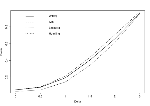
Figure 4: Power ($\alpha=0.05$) simulation results of the WTPS, ATS, Lecoutre and Hotelling for normal distribution and $t=4$ repeated measures under a trend alternative $\boldsymbol{\mu}=(\boldsymbol{\mu}_{1}^{\prime},\boldsymbol{\mu}_{2}^{\prime})^{\prime}=({\bf 0}^{\prime},\delta\boldsymbol{c}^{\prime})^{\prime}$ with $\delta=\{0,0.5,1,1.5,2,3\}$ and $c_{s}=\frac{s}{t},s=1,\ldots,t$.

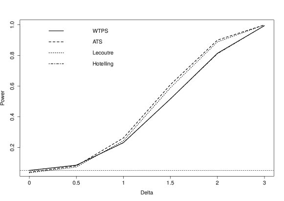
Figure 5: Power ($\alpha=0.05$) simulation results of the WTPS, ATS, Lecoutre and Hotelling for normal distribution and $t=8$ repeated measures under a trend alternative $\boldsymbol{\mu}=(\boldsymbol{\mu}_{1}^{\prime},\boldsymbol{\mu}_{2}^{\prime})^{\prime}=({\bf 0}^{\prime},\delta\boldsymbol{c}^{\prime})^{\prime}$ with $\delta=\{0,0.5,1,1.5,2,3\}$ and $c_{s}=\frac{s}{t},s=1,\ldots,t$.

Figure 6: Power ($\alpha=0.05$) simulation results of the WTPS, ATS, Lecoutre and Hotelling for log-normal distribution and $t=4$ repeated measures under a trend alternative $\boldsymbol{\mu}=(\boldsymbol{\mu}_{1}^{\prime},\boldsymbol{\mu}_{2}^{\prime})^{\prime}=({\bf 0}^{\prime},\delta\boldsymbol{c}^{\prime})^{\prime}$ with $\delta=\{0,0.5,1,1.5,2,3\}$ and $c_{s}=\frac{s}{t},s=1,\ldots,t$.

Figure 7: Power ($\alpha=0.05$) simulation results of the WTPS, ATS, Lecoutre and Hotelling for log-normal distribution and $t=8$ repeated measures under a trend alternative $\boldsymbol{\mu}=(\boldsymbol{\mu}_{1}^{\prime},\boldsymbol{\mu}_{2}^{\prime})^{\prime}=({\bf 0}^{\prime},\delta\boldsymbol{c}^{\prime})^{\prime}$ with $\delta=\{0,0.5,1,1.5,2,3\}$ and $c_{s}=\frac{s}{t},s=1,\ldots,t$.

12 Analysis of the data example: Comparing the different approaches

We again consider the data example from Section 5 on the oxygen consumption of leukocytes. First of all, we notice that the empirical covariance matrices of the two groups appear to be quite different. The empirical covariance matrix in the Placebo-group (rounded to three digits) is given as

$$\left(\begin{array}[]{cccccc}0.025&-0.022&-0.004&0.009&0.015&0.025\\ -0.022&0.092&-0.005&-0.001&-0.024&-0.035\\ -0.004&-0.005&0.081&-0.013&-0.010&-0.004\\ 0.009&-0.001&-0.013&0.037&0.044&0.038\\ 0.015&-0.024&-0.010&0.044&0.069&0.063\\ 0.025&-0.035&-0.004&0.038&0.063&0.115\\ \end{array}\right)$$

whereas in the Verum-group we have

$$\left(\begin{array}[]{cccccc}0.043&0.012&0.046&0.033&0.014&0.055\\ 0.012&0.113&0.008&0.009&0.060&0.032\\ 0.046&0.008&0.065&0.041&0.005&0.066\\ 0.033&0.009&0.041&0.047&0.016&0.059\\ 0.014&0.060&0.005&0.016&0.058&0.047\\ 0.055&0.032&0.066&0.059&0.047&0.116\end{array}\right)$$

Thus, the assumption of homoscedasticity is not fulfilled in this data example.

The results of the analyses using the different methods are presented in the following table. The asymptotic results are again obtained by considering the corresponding $F(\hat{\nu},\infty)$-quantile for the ATS and the $\chi^{2}_{f}$-quantile for the WTS.

Table 14: p-values of the analysis of the $O_{2}$ consumption data.

	ATS			WTS
	asymptotic	PBS	NPBS	asymptotic	Permutation	PBS	NPBS
A	0.001	0.003	$<$0.001	0.001	0.002	0.004	0.005
B	$<$0.001	0.001	0.001	$<$0.001	$<$0.001	0.001	0.001
T	$<$0.001	$<$0.001	$<$0.001	$<$0.001	$<$0.001	$<$0.001	$<$0.001
AB	0.110	0.130	0.140	0.110	0.118	0.125	0.136
AT	0.009	0.012	0.005	$<$0.001	0.001	$<$0.001	$<$0.001
BT	0.094	0.088	0.103	0.115	0.147	0.161	0.157
ABT	0.117	0.154	0.116	0.116	0.162	0.153	0.141

For this data set, the results are similar for all resampling methods and the asymptotic approaches considered.

References

- Ahmad et al. (2008) Ahmad, M. R., Werner, C. and Brunner, E. (2008). Analysis of High Dimensional Repeated Measures Designs: The One Sample Case. Computational Statistics and Data Analysis, 53, 416–427.
- Box (1954) Box, G. E. P. (1954). Some theorems on quadratic forms applied in the study of analysis of variance problems, I. Effect of inequality of variance in the one-way classification. The Annals of Mathematical Statistics, 25, 290–302.
- Brombin et al. (2013) Brombin, C., Midena, E. and Salmaso, L. (2013). Robust non-parametric tests for complex-repeated measures problems in ophthalmology. Statistical Methods in Medical Research, 22, 643–660.
- Brunner (2001) Brunner, E. (2001). Asymptotic and Approximate Analysis of Repeated Measures Designs under Heteroscedasticity. In: Mathematical Statistics with Applications to Biometry, Eds: J. Kunert and G. Trenkler, Josef Eul Verlag, Köln.
- Brunner (2009) Brunner, E. (2009). Repeated Measures under Non-Sphericity. Proceedings of the 6th St.Petersburg Workshop on Simulation, 605–609.
- Brunner et al. (2012) Brunner, E., Bathke, A. C. and Placzek, M. (2012). Estimation of Box’s for low- and high-dimensional repeated measures designs with unequal covariance matrices. Biometrical Journal, 54, 301–316.
- Brunner et al. (2009) Brunner, E., Becker, B. M. and Werner, C. (2009). Approximate Distributions of Quadratic Forms in High-Dimensional Repeated-Measures Designs. Technical Report, Dept. Medical Statistics, University of Göttingen.
- Chi et al. (2012) Chi, Y.-Y., Gribbin, M., Lamers, Y., Gregory, J. F. and Muller, K. E. (2012). Global hypothesis testing for high-dimensional repeated measures outcomes. Statistics in Medicine, 31, 724–742.
- Chung and Romano (2013) Chung, E. and Romano, J. P. (2013). Exact and asymptotically robust permutation tests. The Annals of Statistics, 41, 484–507.
- Corain and Salmaso (2015) Corain, L. and Salmaso, L. (2015). Improving power of multivariate combination-based permutation tests. Statistics and Computing, 25, 203–214.
- Davis (2002) Davis, C.S. (2002). Statistical Methods for the Analysis of Repeated Measurements. Springer, New York.
- Friedrich et al. (2015) Friedrich, S., Konietschke, F. and Pauly, M. (2015). GFD: Tests for General Factorial Designs. R package version 0.2.2.
- Friedrich et al. (2016) Friedrich, S., Brunner, E. and Pauly, M. (2016). Supplement to Permuting Longitudinal Data Despite All The Dependencies.
- Geisser and Greenhouse (1958) Geisser, S. and Greenhouse, S. W. (1958). An Extension of Box’s Result on the Use of the Distribution in Multivariate Analysis. Annals of Mathematical Statistics, 29, 885–891.
- Greenhouse and Geisser (1959) Greenhouse, S. W. and Geisser, S. (1959). On Methods in the Analysis of Profile Data. Psychometrika, 24, 95–112.
- Hájek et al. (1999) Hájek, J. , Šidák, Z. and Sen, P. K. (1999). Theory of Rank Tests. Academic Press, San Diego.
- Hotelling (1931) Hotelling, H. (1931). A generalization of Student’s ratio. Annals of Mathematical Statistics, 2, 360–378.
- Huang et al. (2006) Huang, Y., Xu, H., Calian, V. and Hsu, J. C. (2006). To permute or not to permute. Bioinformatics, 22, 2244–2248.
- Huynh and Feldt (1976) Huynh, H. and Feldt, L. S. (1976). Estimation of the Box Correction for Degrees of Freedom From Sample Data in Randomized Block and Split-Plot Designs. Journal of Educational Statistics, 1, 69–82.
- Janssen (1997) Janssen, A. (1997). Studentized permutation tests for non-i.i.d. hypotheses and the generalized Behrens-Fisher problem. Statistics and Probability Letters, 36, 9–21.
- Janssen and Pauls (2003) Janssen, A. and Pauls, T. (2003). How do bootstrap and permutation tests work?. Annals of Statistics, 768–806.
- Janssen (2005) Janssen, A. (2005). Resampling Student’s t-Type Statistics. Annals of the Institute of Statistical Mathematics, 57, 507–529.
- Kenward and Roger (2009) Kenward, M.G., and Roger, J. H. (2009). An improved approximation to the precision of fixed effects from restricted maximum likelihood. Computational Statistics & Data Analysis 53, 2583–2595.
- Keselman et al. (2000) Keselman, H. J. et al. (2000). Testing treatment effects in repeated measures designs: Trimmed means and bootstrapping. British Journal of Mathematical and Statistical Psychology, 53, 175–191.
- Konietschke and Pauly (2014) Konietschke, F. and Pauly, M. (2014). Bootstrapping and permuting paired t-test type statistics. Statistics and Computing, 24, 283–296.
- Konietschke et al. (2015) Konietschke, F., Bathke, A. C., Harrar, S. W. and Pauly, M. (2015). Parametric and Nonparametric Bootstrap Methods for General MANOVA. Journal of Multivariate Analysis 140, 291–301.
- Lecoutre (1991) Lecoutre, B. (1991). A Correction for the Approximative Test in Repeated Measures Designs With Two or More Independent Groups. Journal of Educational Statistics, 16, 371–372.
- Mathai and Provost (1992) Mathai, A. M. and Provost, S. B. (1992). Quadratic Forms in Random Variables. Marcel Dekker Inc., New York.
- Mielke and Berry (2007) Mielke Jr., P. W. and Berry, K. J. (2007). Permutation Methods: A distance function Approach. Springer.
- Neuhaus (1993) Neuhaus, G. (1993). Conditional rank tests for the two-sample problem under random censorship. Annals of Statistics, 21, 1760–1779.
- Omelka and Pauly (2012) Omelka, M. and Pauly, M. (2012). Testing equality of correlation coefficients in an potentially unbalanced two-sample problem via permutation methods. Journal of Statistical Planning and Inference, 142, 1396–1406.
- Pauly (2011) Pauly, M. (2011). Weighted resampling of martingale difference arrays with applications. Electronic Journal of Statistics, 5, 41–52.
- Pauly et al. (2015a) Pauly, M., Brunner, E. and Konietschke, F. (2015a). Asymptotic Permutation Tests in General Factorial Designs. Journal of the Royal Statistical Society - Series B, 77, 461–473.
- Pauly et al. (2015b) Pauly, M., Ellenberger, D. and Brunner, E. (2015b). Analysis of High-Dimensional One Group Repeated Measures Designs. Statistics, 49(6), 1243–1261.
- Pesarin (2001) Pesarin, F. (2001). Multivariate permutation tests. With applications in biostatistics. Wiley Series in Probability and Statistics.
- Pesarin and Salmaso (2010a) Pesarin, F. and Salmaso, L. (2010a). Permutation Tests for Complex Data. Wiley Series in Probability and Statistics.
- Pesarin and Salmaso (2010b) Pesarin, F. and Salmaso, L. (2010b). Finite-sample consistency of combination-based permutation tests with application to repeated measures designs. Journal of Nonparametric Statistics, 22, 669–684.
- Pesarin and Salmaso (2012) Pesarin, F. and Salmaso, L. (2012). A review and some new results on permutation testing for multivariate problems. Statistics and Computing 22, 639–646.
- Rao and Mitra (1971) Rao, C. R. and Mitra, S. K. (1971). Generalized Inverse of Matrices and Its Applications. Wiley, New York.
- Suo et al. (2013) Suo, C., Toulopoulou, T., Bramon, E., Walshe, M., Picchioni, M., Murray, R. and Ott, J. (2013). Analysis of multiple phenotypes in genome-wide genetic mapping studies, BMC Bioinformatics, 14, 151.
- Vallejo and Ato (2006) Vallejo, G. and Ato, M. (2006). Modified Brown-Forsythe procedure for testing interaction effects in split-plot designs. Multivariate Behavioral Research, 41, 549-578.
- Verbeke (2009) Verbeke, G. and Molenberghs, G. (2009). Linear mixed models for longitudinal data. Springer Science Business Media.
- Verbeke (2012) Verbeke, G. and Molenberghs, G. (2012). Models for discrete longitudinal data. Springer Science Business Media.
- Werner (2004) Werner, C. (2004). Dimensionsstabile Approximation für Verteilungen von quadratischen Formen im Repeated-Measures-Design. Technical Report, Dept. Medical Statistics, University of Göttingen.
- Wilks (1932) Wilks, S. S. (1932). Certain generalizations in the analysis of variance. Biometrika, 24, 471–494.
- Xu and Cui (2008) Xu, J. and Cui, X. (2008). Robustified MANOVA with applications in detecting differentially expressed genes from oligonucleotide arrays. Bioinformatics, 24, 1056–1062.
Supplement To

References

- (1)
- Hájek et al. (1999) Hájek, J. , Šidák, Z. and Sen, P. K. (1999). Theory of Rank Tests. Academic Press, San Diego.
- Hotelling (1931) Hotelling, H. (1931). A generalization of Student’s ratio. Annals of Mathematical Statistics, 2, 360–378.
- Konietschke et al. (2015) Konietschke, F., Bathke, A. C., Harrar, S. W. and Pauly, M. (2015). Parametric and Nonparametric Bootstrap Methods for General MANOVA. Journal of Multivariate Analysis 140, 291–301.
- Lecoutre (1991) Lecoutre, B. (1991). A Correction for the Approximative Test in Repeated Measures Designs With Two or More Independent Groups. Journal of Educational Statistics, 16, 371–372.
- Pauly (2011) Pauly, M. (2011). Weighted resampling of martingale difference arrays with applications. Electronic Journal of Statistics, 5, 41–52.
- Pauly et al. (2015a) Pauly, M., Brunner, E. and Konietschke, F. (2015a). Asymptotic Permutation Tests in General Factorial Designs. Journal of the Royal Statistical Society - Series B, 77, 461–473.
- Rao and Mitra (1971) Rao, C. R. and Mitra, S. K. (1971). Generalized Inverse of Matrices and Its Applications. Wiley, New York.