Vanishing cycles and Cartan eigenvectors

Abstract

Using the ideas coming from the singularity theory, we study the eigenvectors of the Cartan matrices of finite root systems, and of $q$-deformations of these matrices.

March 10, 2024

1 Introduction

Let $A(R)$ be the Cartan matrix of a finite root system $R$. The coordinates of its eigenvectors have an important meaning in the physics of integrable systems; we will say more on this below.

The aim of this note is to study these numbers and their $q$-deformations, using some results coming from the singularity theory.

We discuss three ideas:

(a) Cartan/Coxeter correspondence;

(b) Sebastiani - Thom product;

(c) Givental’s $q$-deformations.

Let us explain what we are talking about.

Let us suppose that $R$ is simply laced, i.e. of type $A,D$, or $E$. These root systems are in one-to-one correspondence with (classes of) simple singularities

$f:\mathbb{C}^{N}\to\mathbb{C}$, cf. AGV . Under this correspondence, the root lattice $Q(R)$ is identified with the lattice of vanishing cycles, and the Cartan matrix $A(R)$ is the intersection matrix with respect to a distinguished base. The action of the Weyl group on $Q(R)$ is realized by Gauss - Manin monodromies - this is the Picard - Lefschetz theory (for some details see §2 below).

Remarkably, this geometric picture provides a finer structure: namely, the symmetric matrix $A=A(R)$ comes equipped with a decomposition

$$A=L+L^{t}$$ (1)

where $L$ is a nondegenerate triangular ”Seifert form”, or ”variation matrix”. The matrix

$$C=-L^{-1}L^{t}$$ (2)

represents a Coxeter element of $R$; geometrically it is the operator of ”classical monodromy”.

We call the relation (1) - (2) between the Cartan matrix and the Coxeter element the Cartan/Coxeter correspondence. It works more generally for non-symmetric $A$ (in this case (1) should be replaced by

$$A=L+U$$ (3)

where $L$ is lower triangular and $U$ is upper triangular), and is due to Coxeter, cf. Co , no. 1, p. 767, see §3 below.

In a particular case (corresponding to a bipartition of the Dynkin graph) this relation is equivalent to an observation by R.Steinberg, cf. Stein , cf. §3.3 below.

This corresppondence allows one to relate the eigenvectors of $A$ and $C$, cf. Theorem 1.

A decomposition (1) will be called a polarization of the Cartan matrix $A$. In 4.1 below we introduce an operation of Sebastiani - Thom, or joint product $A*B$ of Cartan matrices (or of polarized lattices) $A$ and $B$. The root lattice of $A*B$ is the tensor product of the root lattice of $A$ and the root lattice of $B$. With respect to this operation the Coxeter eigenvectors factorize very simply.

For example, the lattices $E_{6}$ and $E_{8}$ decompose into three ”quarks”:

$$E_{6}=A_{3}*A_{2}*A_{1}$$ (4)

$$E_{8}=A_{4}*A_{2}*A_{1}$$ (5)

These decompositions are the main message from the singularity theory, and we discuss them in detail in this note.

We use (4), (5), and the Cartan/Coxeter correspondence to get expressions for all Cartan eigenvectors of $E_{6}$ and $E_{8}$; this is the first main result of this note, see 4.9, 4.11 below.

(An elegant expression for all the Cartan eigenvectors of all finite root systems was given by P.Dorey, cf. D (a), Table 2 on p. 659.)

In the paper Giv , A. Givental has proposed a $q$-twisted version of the Picard - Lefschetz theory, which gave rise to a $q$-deformation of $A$,

$$A(q)=L+qL^{t}.$$ (6)

Again, as Givental remarked, the decomposition (3) allows us to drop the assumption of symmetry in the definition above. In the last section, §5, we calculate the eigenvalues and eigenvectors of $A(q)$ in terms of the eigenvalues and eigenvectors of $A$. This is the second main result of this note.

It turns out that if $\lambda$ is an eigenvalue of $A$ then

$$\lambda(q)=1+(\lambda-2)\sqrt{q}+q$$ (7)

will be an eigenvalue of $A(q)$. The coordinates of the corresponding eigenvector $v(q)$ are obtained from the coordinates of $v=v(1)$ by multiplication by appropriate powers of $q$; this is related to the fact that the Dynkin graph of $A$ is a tree, cf. 5.2. For an example of $E_{8}$, see (26).

In physics, the coordinates of the Perron - Frobenius Cartan eigenvectors appear as particle masses in affine Toda field theories, cf. D ; F and the Section LABEL:toda below.

In a pioneering paper Z , A. B. Zamolodchikov has discovered an octuplet of particles of $E_{8}$ symmetry in the two-dimensional critical Ising model in a magnetic field, and calculated their masses, cf. the Sections 4.10 and LABEL:sub64.

The Appendix outlines some of the results of a neutron scattering experiment Coldea , where the two lowest-mass $E_{8}$ particles of the Zamolodchikov’s theory may have been observed.

2 Recollections from the singularity theory

Here we recall some classical constructions and statements, cf. AGV .

2.1 Lattice of vanishing cycles

Let $f:\ (\mathbb{C}^{N},0)\to(\mathbb{C},0)$ be the germ of a holomorphic function with an isolated critical point at $0$, with $f(0)=0$. We will be interested only in polynomial functions (from the list below, cf. §2.4), so $f\in\mathbb{C}[x_{1},\ldots,x_{N}]$. The Milnor ring of $f$ is defined by

$$\operatorname{Miln}(f,0)=\mathbb{C}[[x_{1},\ldots,x_{N}]]/(\partial_{1}f,\ldots,\partial_{N}f)$$

where $\partial_{i}:=\partial/\partial x_{i}$; it is a finite-dimensional commutative $\mathbb{C}$-algebra. (In fact, it is a Frobenius, or, equivalently, a Gorenstein algebra.) The number

$$\mu:=\dim_{\mathbb{C}}\operatorname{Miln}(f,0)$$

is called the multiplicity or Milnor number of $(f,0)$.

A Milnor fiber is

$$V_{z}=f^{-1}(z)\cap\bar{B}_{\rho}$$

where

$$\bar{B}_{\rho}=\{(x_{1},\ldots,x_{N})|\ \sum|x_{i}|^{2}\leq\rho\}$$

for $1\gg\rho\gg|z|>0$.

For $z$ belonging to a small disc $D_{\epsilon}=\{z\in\mathbb{C}|\ |z|<\epsilon\}$, the space $V_{z}$ is a complex manifold with boundary, homotopically equivalent to a bouquet $\vee S^{N-1}$ of $\mu$ spheres, M .

The family of free abelian groups

$$Q(f;z):=\tilde{H}_{N-1}(V_{z};\mathbb{Z})\overset{\sim}{=}\mathbb{Z}^{\mu},\ z\in\overset{\bullet}{D}_{\epsilon}:=D_{\epsilon}\setminus\{0\},$$ (8)

($\tilde{H}$ means that we take the reduced homology for $N=1$), carries a flat Gauss - Manin conection.

Take $t\in\mathbb{R}_{>0}\cap\overset{\bullet}{D}_{\epsilon}$; the lattice $Q(f;t)$ does not depend, up to a canonical isomorphism, on the choice of $t$. Let us call this lattice $Q(f)$. The linear operator

$$T(f):Q(f)\overset{\sim}{\longrightarrow}Q(f)$$ (9)

induced by the path $p(\theta)=e^{i\theta}t,\ 0\leq\theta\leq 2\pi$, is called the classical monodromy of the germ $(f,0)$.

In all the examples below $T(f)$ has finite order $h$. The eigenvalues of $T(f)$ have the form $e^{2\pi ik/h},\ k\in\mathbb{Z}$. The set of suitably chosen $k$’s for each eigenvalue are called the spectrum of our singularity.

2.2 Morse deformations

The $\mathbb{C}$-vector space $\operatorname{Miln}(f,0)$ may be identified with the tangent space to the base $B$ of the miniversal defomation of $f$. For

$$\lambda\in B^{0}=B\setminus\Delta$$

where $\Delta\subset B$ is an analytic subset of codimension $1$, the corresponding function $f_{\lambda}:\mathbb{C}^{N}\to\mathbb{C}$ has $\mu$ nondegenerate Morse critical points with distinct critical values, and the algebra $\operatorname{Miln}(f_{\lambda})$ is semisimple, isomorphic to $\mathbb{C}^{\mu}$.

Let $0\in B$ denote the point corresponding to $f$ itself, so that $f=f_{0}$, and pick $t\in\mathbb{R}_{>0}\cap\overset{\bullet}{D}_{\epsilon}$ as in §2.1.

Afterwards pick $\lambda\in B^{0}$ close to $0$ in such a way that the critical values $z_{1},\ldots z_{\mu}$ of $f_{\lambda}$ have absolute values $\ll t$.

As in §2.1, for each

$$z\in\tilde{D}_{\epsilon}:=D_{\epsilon}\setminus\{z_{1},\ldots z_{\mu}\}$$

the Milnor fiber $V_{z}$ has the homotopy type of a bouquet $\vee S^{N-1}$ of $\mu$ spheres, and we will be interested in the middle homology

$$Q(f_{\lambda};z)=\tilde{H}_{N-1}(V_{z};\mathbb{Z})\overset{\sim}{=}\mathbb{Z}^{\mu}$$

The lattices $Q(f_{\lambda};z)$ carry a natural bilinear product induced by the cup product in the homology which is symmetric (resp. skew-symmetric) when $N$ is odd (resp. even).

The collection of these lattices, when $z\in\tilde{D}_{\epsilon}$ varies, carries a flat Gauss - Manin connection.

Consider an ”octopus”

$$Oct(t)\subset\mathbb{C}$$

with the head at $t$: a collection of non-intersecting paths $p_{i}$ (”tentacles”) connecting $t$ with $z_{i}$ and not meeting the critical values $z_{j}$ otherwise. It gives rise to a base

$$\{b_{1},\ldots,b_{\mu}\}\subset Q(f_{\lambda}):=Q(f_{\lambda};t)$$

(called ”distinguished”) where $b_{i}$ is the cycle vanishing when being transferred from $t$ to $z_{i}$ along the tentacle $p_{i}$, cf. Gab , AGV .

The Picard - Lefschetz formula describes the action of the fundamental group $\pi_{1}(\tilde{D}_{\epsilon};t)$ on $Q(f_{\lambda})$ with respect to this basis. Namely, consider a loop $\gamma_{i}$ which turns around $z_{i}$ along the tentacle $p_{i}$, then the corresponding transformation of $Q(f_{\lambda})$ is the reflection (or transvection) $s_{i}:=s_{b_{i}}$, cf. Lef , Théorème fondamental, Ch. II, p. 23.

The loops $\gamma_{i}$ generate the fundamental group $\pi_{1}(\tilde{D}_{\epsilon})$. Let

$$\rho:\ \pi_{1}(\tilde{D}_{\epsilon};t)\to GL(Q(f_{\lambda}))$$

denote the monodromy representation. The image of $\rho$, denoted by $G(f_{\lambda})$ and called the monodromy group of $f_{\lambda}$, lies inside the subgroup
$O(Q(f_{\lambda}))\subset GL(Q(f_{\lambda}))$ of linear transformations respecting the above mentioned bilinear form on $Q(f_{\lambda})$.

The subgroup $G(f_{\lambda})$ is generated by $s_{i},1\leq i\leq\mu$.

As in §2.1, we have the monodromy operator

$$T(f_{\lambda})\in G(f_{\lambda}),$$

the image by $\rho$ of the path $p\subset\tilde{D}_{\epsilon}$ starting at $t$ and going around all points $z_{1},\ldots,z_{\mu}$.

This operator $T(f_{\lambda})$ is now a product of $\mu$ simple reflections

$$T(f_{\lambda})=s_{1}s_{2}\ldots s_{\mu},$$

- this is because the only critical value $0$ of $f$ became $\mu$ critical values $z_{1},\ldots,z_{\mu}$ of $f_{\lambda}$.

One can identify the relative (reduced) homology $\tilde{H}_{N-1}(V_{t},\partial V_{t};\mathbb{Z})$ with the dual group $\tilde{H}_{N-1}(V_{t};\mathbb{Z})^{*}$, and one defines a map

$$\text{var}:\tilde{H}_{N-1}(V_{t},\partial V_{t};\mathbb{Z})\to\tilde{H}_{N-1}(V_{t};\mathbb{Z}),$$

called a variation operator, which translates to a map

$$L:Q(f_{\lambda})^{*}\overset{\sim}{\longrightarrow}Q(f_{\lambda})$$

(”Seifert form”) such that the matrix $A(f_{\lambda})$ of the bilinear form in the distinguished basis is

$$A(f_{\lambda})=L+(-1)^{N-1}L^{t},$$

and

$$T(f_{\lambda})=(-1)^{N-1}LL^{-t}.$$

A choice of a path $q$ in $B$ connecting $0$ with $\lambda$, enables one to identify $Q(f)$ with $Q(f_{\lambda})$, and $T(f)$ will be identified with $T(f_{\lambda})$.

The image $G(f)$ of the monodromy group $G(f_{\lambda})$ in $GL(Q(f))\overset{\sim}{=}GL(Q(f_{\lambda}))$ is called the monodromy group of $f$; it does not depend on a choice of a path $q$.

2.3 Sebastiani - Thom factorization

If $g\in\mathbb{C}[y_{1},\ldots,y_{M}]$ is another function, the sum, or join of two singularities $f\oplus g:\ \mathbb{C}^{N+M}\to\mathbb{C}$ is defined by

$$(f\oplus g)(x,y)=f(x)+g(y)$$

Obviously we can identify

$$\operatorname{Miln}(f\oplus g)\overset{\sim}{=}\operatorname{Miln}(f)\otimes\operatorname{Miln}(g)$$

Note that the function $g(y)=y^{2}$ is a unit for this operation.

It follows that the singularities $f(x_{1},\ldots,x_{N})$ and

$$f(x_{1},\ldots,x_{N})+x_{M+1}^{2}+\ldots+x^{2}_{N+M}$$

are ”almost the same”. In order to have good signs (and for other purposes) it is convenient to add some squares to a given $f$ to get $N\equiv 3\mod(4)$.

The fundamental Sebastiani - Thom theorem, ST , says that there exists a natural isomorphism of lattices

$$Q(f\oplus g)\overset{\sim}{=}Q(f)\otimes_{\mathbb{Z}}Q(g),$$

and under this identification the full monodromy decomposes as

$$T_{f\oplus g}=T_{f}\otimes T_{g}$$

Thus, if

$$\operatorname{Spec}(T_{f})=\{e^{\mu_{p}\cdot 2\pi i/h_{1}}\},\ \operatorname{Spec}(T_{f})=\{e^{\nu_{q}\cdot 2\pi i/h_{2}}\}$$

then

$$\operatorname{Spec}(T_{f\oplus g})=\{e^{(\mu_{p}h_{2}+\nu_{q}h_{1})\cdot 2\pi i/h_{1}h_{2}}\}$$

2.4 Simple singularities

Cf. AGV (a), 15.1. They are:

$$x^{n+1},\ n\geq 1,$$

$$x^{2}y+y^{n-1},\ n\geq 4$$

$$x^{4}+y^{3}$$

$$xy^{3}+x^{3}$$

$$x^{5}+y^{3}$$

Their names come from the following facts:

— their lattices of vanishing cycles may be identified with the corresponding root lattices;

— the monodromy group is identified with the corresponding Weyl group;

— the classical monodromy $T_{f}$ is a Coxeter element, therefore its order $h$ is equal to the Coxeter number, and

$$\operatorname{Spec}(T_{f})=\{e^{2\pi ik_{1}/h},\ldots,e^{2\pi ik_{r}/h}\}$$

where the integers

$$1=k_{1}<k_{2}<\ldots<k_{r}=h-1,$$

are the exponents of our root system.

We will discuss the case of $E_{8}$ in some details below.

3 Cartan - Coxeter correspondence

3.1 Lattices, polarization, Coxeter elements

Let us call a lattice a pair $(Q,A)$ where $Q$ is a free abelian group, and

$$A:Q\times Q\to\mathbb{Z}$$

a symmetric bilinear map (”Cartan matrix”). We shall identify $A$ with a map

$$A:Q\to Q^{\vee}:=Hom(Q,\mathbb{Z}).$$

A polarized lattice is a triple $(Q,A,L)$ where $(Q,A)$ is a lattice, and

$$L:\ Q\overset{\sim}{\longrightarrow}Q^{\vee}$$

(”variation”, or ”Seifert matrix”) is an isomorphism such that

$$A=A(L):=L+L^{\vee}$$ (10)

where

$$L^{\vee}:Q=Q^{\vee\vee}\overset{\sim}{\longrightarrow}Q^{\vee}$$

is the conjugate to $L$.

The Coxeter automorphism of a polarized lattice is defined by

$$C=C(L)=-L^{-1}L^{\vee}\in GL(Q).$$ (11)

We shall say that the operators $A$ and $C$ are in a Cartan - Coxeter correspondence.

Example Let $(Q,A)$ be a lattice, and $\{e_{1},\ldots,e_{n}\}$ an ordered $\mathbb{Z}$-base of $Q$. With respect to this base $A$ is expressed as a symmetric matrix $A=(a_{ij})=A(e_{i},e_{j})\in\mathfrak{gl}_{n}(\mathbb{Z})$. Let us suppose that all $a_{ii}$ are even. We define the matrix of $L$ to be the unique upper triangular matrix $(\ell_{ij})$ such that $A=L+L^{t}$ (in particular $\ell_{ii}=a_{ii}/2$; in our examples we will have $a_{ii}=2$.) We will call $L$ the standard polarization associated to an ordered base. $\square$

Polarized lattices form a groupoid:

an isomorphosm of polarized lattices $f:\ (Q_{1},A_{1},L_{1})\overset{\sim}{\longrightarrow}(Q_{2},A_{2},L_{2})$ is by definition an isomorphism of abelian groups $f:Q_{1}\overset{\sim}{\longrightarrow}Q_{2}$ such that

$$L_{1}(x,y)=L_{2}(f(x),f(y))$$

(and whence $A_{1}(x,y)=A_{2}(f(x),f(y))$).

3.2 Orthogonality

Lemma 1

(i) (orthogonality)

$$A(x,y)=A(Cx,Cy).$$

(ii) (gauge transformations) For any $P\in GL(Q)$

$$A(P^{\vee}LP)=P^{\vee}A(L)P,\ C(P^{\vee}LP)=P^{-1}C(L)P.$$

$\square$

3.3 Black/white decomposition and a Steinberg’s theorem

Cf. Stein , C . Let $\alpha_{1},\ldots,\alpha_{r}$ be a base of simple roots of a finite reduced irreducible root system $R$ (not necessarily simply laced).

Let

$$A=(a_{ij})=(\langle\alpha_{i},\alpha_{j}^{\vee}\rangle)$$

be the Cartan matrix.

Choose a black/white coloring of the set of vertices of the corresponding Dynkin graph $\Gamma(R)$ in such a way that any two neighbouring vertices have different colours; this is possible since $\Gamma(R)$ is a tree (cf. 5.2).

Let us choose an ordering of simple roots in such a way that the first $p$ roots are black, and the last $r-p$ roots are white. In this base $A$ has a block form

$$A=\left(\begin{matrix}2I_{p}&X\\ Y&2I_{r-p}\end{matrix}\right)$$

Consider a Coxeter element

$$C=s_{1}s_{2}\ldots s_{r}=C_{B}C_{W},$$ (12)

where

$$C_{B}=\prod_{i=1}^{p}s_{i},\ C_{W}=\prod_{i=p+1}^{r}s_{i}.$$

Here $s_{i}$ denotes the simple reflection corresponding to the root $\alpha_{i}$.

The matrices of $C_{B},C_{W}$ with respect to the base $\{\alpha_{i}\}$ are

$$C_{B}=\left(\begin{matrix}-I&-X\\ 0&I\end{matrix}\right),C_{W}=\left(\begin{matrix}I&0\\ -Y&-I\end{matrix}\right),$$

so that

$$C_{B}+C_{W}=2I-A.$$ (13)

This is an observation due to R.Steinberg, cf. Stein , p. 591.

We can also rewrite this as follows. Set

$$L=\left(\begin{matrix}I&0\\ Y&I\end{matrix}\right),\ U=\left(\begin{matrix}I&X\\ 0&I\end{matrix}\right).$$

Then $A=L+U$, and one checks easily that

$$C=-U^{-1}L,$$ (14)

so we are in the situation 3.1. This explains the name ”Cartan - Coxeter coresspondence”.

3.4 Eigenvectors’ correspondence

Theorem 3.1

Let

$$L=\left(\begin{matrix}I_{p}&0\\ Y&I_{r-p}\end{matrix}\right),\ U=\left(\begin{matrix}I_{p}&X\\ 0&I_{r-p}\end{matrix}\right)\$$

be block matrices. Set

$$A=L+U,\ C=-U^{-1}L.$$

Let $\mu\neq 0$ be a complex number, $\sqrt{\mu}$ be any of its square roots, and

$$\lambda=2-\sqrt{\mu}-1/\sqrt{\mu}.$$ (15)

Then a vector $v_{C}=\left(\begin{matrix}v_{1}\\ v_{2}\end{matrix}\right)$ is an eigenvector of $C$ with eigenvalue $\mu$ if and only if

$$v_{A}=\left(\begin{matrix}v_{1}\\ \sqrt{\mu}v_{2}\end{matrix}\right)$$

is an eigenvector of $A$ with the eigenvalue $\lambda$.

Proof: a direct check. $\square$

3.4.1 Remark

Note that the formula (15) gives two possible values of $\lambda$ corresponding to $\pm\sqrt{\mu}$. On the other hand, $\lambda$ does not change if we replace $\mu$ by $\mu^{-1}$.

In the simplest case of $2\times 2$ matrices the eigenvalues of $A$ are $2\pm(\sqrt{\mu}+\sqrt{\mu^{-1}})$, whereas the eigenvalues of $C$ are $\mu^{\pm 1}$.

Corollary 1

In the notations of 3.1, a vector

$$x=\sum x_{j}\alpha_{j}$$

is an eigenvector of $A$ with the eigenvalue $2(1-\cos\theta)$ iff the vector

$$x_{c}:=\sum e^{\pm i\theta/2}x_{j}\alpha_{j}$$

where the sign in $e^{\pm i\theta/2}$ is plus if $i$ is a white vertex, and minus otherwise, is an eigenvector of $C$ with eigenvalue $e^{2i\theta}$.

Cf. F.

Proof

Without loss of generality, we can suppose that $A$ is expressed in a basis of simple roots such that the first $r-p$ ones are white, and the last $p$ roots are black.

Then $A$ has a block form

$$A=\begin{pmatrix}2I_{r-p}&X\\ Y&2I_{p}\end{pmatrix}=\begin{pmatrix}I_{r-p}&0\\ Y&I_{p}\end{pmatrix}+\begin{pmatrix}I_{r-p}&X\\ 0&I_{p}\end{pmatrix}=L+U$$

Applying Theorem 1 with

$$v_{1}=\begin{pmatrix}e^{i\theta/2}x_{1}\\ ..\\ e^{i\theta/2}x_{r-p}\end{pmatrix}\text{ and }v_{2}=\begin{pmatrix}e^{-i\theta/2}x_{r-p+1}\\ ..\\ e^{-i\theta/2}x_{r}\end{pmatrix}$$

and the well-known eigenvalues of the Cartan matrix $A$,

$$\lambda=2-2\cos\theta_{k},\text{ with }\theta_{k}=2\pi k/h,k\in\operatorname{Exp}(R)$$

we obtain : $x_{c}:=\sum e^{\pm i\theta/2}x_{j}\alpha_{j}$ is an eigenvector of $C$ with the eigenvalue $e^{2i\theta_{k}}$ iff $e^{i\theta_{k}}x=e^{i\theta_{k}}\sum x_{j}\alpha_{j}$ is an eigenvector of $A$ with the eigenvalue $2-2\cos\theta_{k}$. $\square$

3.5 Example: the root systems $A_{n}$.

We consider the Dynkin graph of $A_{n}$ with the obvious numbering of the vertices.

The Coxeter number $h=n+1$, the set of exponents:

$$\operatorname{Exp}(A_{n})=\{1,2,\ldots,n\}$$

The eigenvalues of any Coxeter element are $e^{i\theta_{k}}$, and the eigenvalues of the Cartan matrix $A(A_{n})$ are $2-2\cos\theta_{k}$, $\theta_{k}=2\pi k/h$, $k\in\operatorname{Exp}(A_{n})$.

An eigenvector of $A(A_{n})$ with the eigenvalue $2-2\cos\theta$ has the form

$$x(\theta)=(\sum_{k=0}^{n-1}e^{i(n-1-2k)\theta},\sum_{k=0}^{n-2}e^{i(n-2-2k)\theta},\ldots,1)$$ (16)

Denote by $C(A_{n})$ the Coxeter element

$$C(A_{n})=s_{1}s_{2}\ldots s_{n}$$

Its eigenvector with the eigenvalue $e^{2i\theta}$ is:

$$X_{C(A_{n})}=(\sum_{k=0}^{n-j}e^{2ik\theta})_{1\leq j\leq n}$$

For example, for $n=4$:

$$C_{A_{4}}=\begin{pmatrix}0&0&0&-1\\ 1&0&0&-1\\ 0&1&0&-1\\ 0&0&1&-1\end{pmatrix}\text{ and }X_{C(A_{4})}=\begin{pmatrix}1+e^{2i\theta}+e^{4i\theta}+e^{6i\theta}\\ 1+e^{2i\theta}+e^{4i\theta}\\ 1+e^{2i\theta}\\ 1\end{pmatrix}$$

is an eigenvector with eigenvalue $e^{2i\theta}$.

Similarly, for $n=2$:

$$C_{A_{2}}=\begin{pmatrix}0&-1\\ 1&-1\end{pmatrix},\ X_{C(A_{2})}=\begin{pmatrix}1+e^{2i\gamma}\\ 1\end{pmatrix}$$

$\square$

4 Sebastiani - Thom product; factorization of $E_{8}$ and $E_{6}$

4.1 Join product

Suppose we are given two polarized lattices $(Q_{i},A_{i},L_{i})$, $i=1,2$.

Set $Q=Q_{1}\otimes Q_{2}$, whence

$$L:=L_{1}\otimes L_{2}:Q\overset{\sim}{\longrightarrow}Q^{\vee},$$

and define

$$A:=A_{1}*A_{2}:=L+L^{\vee}:Q\overset{\sim}{\longrightarrow}Q^{\vee}$$

The triple $(Q,A,L)$ will be called the join, or Sebastiani - Thom, product of the polarized lattices $Q_{1}$ and $Q_{2}$, and denoted by $Q_{1}*Q_{2}$.

Obviously

$$C(L)=-C(L_{1})\otimes C(L_{2})\in GL(Q_{1}\otimes Q_{2}).$$

It follows that if $\operatorname{Spec}(C(L_{i}))=\{e^{2\pi ik_{i}/h_{i}},\ k_{i}\in K_{i}\}$ then

$$\operatorname{Spec}(C(L))=\{-e^{2\pi i(k_{1}/h_{1}+k_{2}/h_{2})},\ (k_{1},k_{2})\in K_{1}\times K_{2}\}$$ (17)

4.2 $E_{8}$ versus $A_{4}*A_{2}*A_{1}$: elementary analysis

The ranks:

$$r(E_{8})=8=r(A_{4})r(A_{2})r(A_{1});$$

the Coxeter numbers:

$$h(E_{8})=h(A_{4})h(A_{2})h(A_{1})=5\cdot 3\cdot 2=30.$$

It follows that

$$|R(E_{8})|=240=|R(A_{4})||R(A_{2})||R(A_{1})|.$$

The exponents of $E_{8}$ are:

$$1,7,13,19,11,17,23,29.$$

All these numbers, except $1$, are primes, and these are all primes $\leq 30$, not dividing $30$.

They may be determined from the formula

$$\frac{i}{5}+\frac{j}{3}+\frac{1}{2}=\frac{30+k(i,j)}{30},\ 1\leq i\leq 4,\ 1\leq j\leq 2,$$

so

$$k(i,1)=1+6(i-1)=1,7,13,19;\$$

$$k(i,2)=1+10+6(i-1)=11,17,23,29.$$

This shows that the exponents of $E_{8}$ are the same as the exponents of
$A_{4}*A_{2}*A_{1}$.

The following theorem is more delicate.

4.3 Decomposition of $Q(E_{8})$

Theorem 4.1

(Gabrielov, cf. Gab , Section 6, Example 3). There exists a polarization of the root lattice $Q(E_{8})$ and an isomorphism of polarized lattices

$$\Gamma:Q(A_{4})*Q(A_{2})*Q(A_{1})\overset{\sim}{\longrightarrow}Q(E_{8}).$$ (18)

In the left hand side $Q(A_{n})$ means the root lattice of $A_{n}$ with the standard Cartan matrix and the standard polarization

$$A(A_{n})=L(A_{n})+L(A_{n})^{t}$$

where the Seifert matrix $L(A_{n})$ is upper triangular.

In the process of the proof, given in §4.4 - 4.6 below, the isomorphism $\Gamma$ will be written down explicitly.

4.4 Beginning of the proof

For $n=4,2,1$, we consider the bases of simple roots $e_{1},\ldots,e_{n}$ in $Q(A_{n})$, with scalar products given by the Cartan matrices $A(A_{n})$.

The tensor product of three lattices

$$Q_{*}=Q(A_{4})\otimes Q(A_{2})\otimes Q(A_{1})$$

will be equipped with the ”factorizable” basis in the lexicographic order:

$$(f_{1},\ldots,f_{8}):=(e_{1}\otimes e_{1}\otimes e_{1},e_{1}\otimes e_{2}\otimes e_{1},e_{2}\otimes e_{1}\otimes e_{1},e_{2}\otimes e_{2}\otimes e_{1},$$

$$e_{3}\otimes e_{1}\otimes e_{1},e_{3}\otimes e_{2}\otimes e_{1},e_{4}\otimes e_{1}\otimes e_{1},e_{4}\otimes e_{2}\otimes e_{1}).$$

Introduce a scalar product $(x,y)$ on $Q_{*}$ given, in the basis $\{f_{i}\}$, by the matrix

$$A_{*}=A_{4}*A_{2}*A_{1}.$$

4.5 Gabrielov - Picard - Lefschetz transformations $\alpha_{m},\beta_{m}$

Let $(Q,(,))$ be a lattice of rank $r$. We introduce the following two sets of transformations $\{\alpha_{m}\},\{\beta_{m}\}$ on the set $Bases-cycl(Q)$ of cyclically ordered bases of $Q$.

If $x=(x_{i})_{i\in\mathbb{Z}/r\mathbb{Z}}$ is a base, and $m\in\mathbb{Z}/r\mathbb{Z}$, we set

$$(\alpha_{m}(x))_{i}=\left\{\begin{matrix}x_{m+1}+(x_{m+1},x_{m})x_{m}\ &\text{if}\ i=m\\ x_{m}&\text{if}\ i=m+1\\ x_{i}&\text{otherwise}\end{matrix}\right.$$

and

$$(\beta_{m}(x))_{i}=\left\{\begin{matrix}x_{m}&\text{if}\ i=m-1\\ x_{m-1}+(x_{m-1},x_{m})x_{m}\ &\text{if}\ i=m\\ x_{i}&\text{otherwise}\end{matrix}\right.$$

We define also a transformation $\gamma_{m}$ by

$$(\gamma_{m}(x))_{i}=\left\{\begin{matrix}-x_{m}&\text{if}\ i=m\\ x_{i}&\text{otherwise}\end{matrix}\right.$$

4.6 Passage from $A_{4}*A_{2}*A_{1}$ to $E_{8}$

Consider the base $f=\{f_{1},\ldots f_{8}\}$ of the lattice $Q_{*}:=Q(A_{4})\otimes Q(A_{2})\otimes Q(A_{1})$ described in §4.4, and apply to it the following transformation

$$G^{\prime}=\gamma_{2}\gamma_{1}\beta_{4}\beta_{3}\alpha_{3}\alpha_{4}\beta_{4}\alpha_{5}\alpha_{6}\alpha_{7}\alpha_{1}\alpha_{2}\alpha_{3}\alpha_{4}\beta_{6}\beta_{3}\alpha_{1},$$ (19)

cf. Gab , Example 3. Note that

$$\gamma_{2}\gamma_{1}=\alpha_{1}^{6},$$ (20)

cf. Br .

Then the base $G^{\prime}(f)$ has the intersection matrix given by the Dynkin graph of $E_{8}$, with the ordering indicated in Figure 1 below.

$$1\ -\ 2\ -\ 3\ -\ 5\ -\ 6\ -\ 7\ -8$$

$$|\ \ \ \ \ \ \ \ \ \ \ \ \$$

$$4\ \ \ \ \ \ \ \ \ \ \ \ \$$

Figure 1: Gabrielov’s ordering of $E_{8}$.

This concludes the proof of Theorem 4.1 $\square$

4.7 The induced map of root sets

By definition, the isomorphism of lattices $\Gamma$, (22), induces a bijection between the bases

$$g:\ \{f_{1},\ldots,f_{8}\}\overset{\sim}{\longrightarrow}\{\alpha_{1},\ldots,\alpha_{8}\}\subset R(E_{8}).$$

where in the right hand side we have the base of simple roots, and a map

$$G:\ R(A_{4})\times R(A_{2})\times R(A_{1})\to R(E_{8}),\ G(x,y,z)=\Gamma(x\otimes y\otimes z)$$

of sets of the same cardinality $240$ which is not a bijection however: its image consists of $60$ elements.

Note that the set of vectors $\alpha\in Q(E_{8})$ with $(\alpha,\alpha)=2$ coincides with the root system $R(E_{8})$, cf. Serre , Première Partie, Ch. 5, 1.4.3.

4.8 Passage to Bourbaki ordering

The isomorphism $G^{\prime}$ (19) is given by a matrix $G^{\prime}\in GL_{8}(\mathbb{Z})$ such that

$$A_{G}(E_{8})=G^{\prime t}A_{*}G^{\prime}$$

where we denoted

$$A_{*}=A(A_{4})*A(A_{2})*A(A_{1}),$$

the factorized Cartan matrix, and $A_{G}$ denotes the Cartan matrix of $E_{8}$ with respect to the numbering of roots indicated on Figure 1.

Now let us pass to the numbering of vertices of the Dynkin graph of type $E_{8}$ indicated in B (the difference with Gabrielov’s numeration is in three vertices $2,3$, and $4$).

$$1\ -\ 3\ -\ 4\ -\ 5\ -\ 6\ -\ 7\ -8$$

$$|\ \ \ \ \ \ \ \ \ \ \ \ \$$

$$2\ \ \ \ \ \ \ \ \ \ \ \ \$$

Figure 2: Bourbaki ordering of $E_{8}$.

The Gabrielov’s Coxeter element (the full monodromy) in the Bourbaki numbering looks as follows:

$$C_{G}(E_{8})=s_{1}\circ s_{3}\circ s_{4}\circ s_{2}\circ s_{5}\circ s_{6}\circ s_{7}\circ s_{8}$$

Lemma 2

Let $A(E_{8})$ be the standard Cartan matrix of $E_{8}$ from [B]:

$$A(E_{8})=\begin{pmatrix}2&0&-1&0&0&0&0&0\\ 0&2&0&-1&0&0&0&0\\ -1&0&2&-1&0&0&0&0\\ 0&-1&-1&2&-1&0&0&0\\ 0&0&0&-1&2&-1&0&0\\ 0&0&0&0&-1&2&-1&0\\ 0&0&0&0&0&-1&2&-1\\ 0&0&0&0&0&0&-1&2\end{pmatrix}.$$

Then

$$A(E_{8})=G^{t}A_{*}G$$

and

$$C_{G}(E_{8})=G^{-1}C_{*}G$$

where

$$C_{*}=C(Q(A_{4})*Q(A_{2})*Q(A_{1}))=C(A_{4})\otimes C(A_{2})\otimes C(A_{1}),$$

is the factorized Coxeter element, and

$$G=\begin{pmatrix}0&0&0&1&-1&0&0&0\\ -1&1&0&0&0&0&0&0\\ 0&0&-1&1&0&0&0&0\\ -1&1&-1&0&0&1&0&0\\ 0&1&-1&0&0&0&1&0\\ -1&1&-1&0&0&0&1&0\\ 0&1&-1&0&0&0&0&1\\ 0&1&-1&0&0&0&0&0\end{pmatrix}$$

Here

$$G=G^{\prime}P$$

where $P$ is the permutation matrix of passage from the Gabrielov’s ordering in Figure 1 to the Bourbaki ordering in Figure 2

4.9 Cartan eigenvectors of $E_{8}$

To obtain the Cartan eigenvectors of $E_{8}$, one should pass from $C_{G}(E_{8})$ to the ”black/white” Coxeter element (as in §3.3)

$$C_{BW}(E_{8})=s_{1}\circ s_{4}\circ s_{6}\circ s_{8}\circ s_{2}\circ s_{3}\circ s_{5}\circ s_{7}$$

Any two Coxeter elements are conjugate in the Weyl group $W(E_{8})$.

The elements $C_{G}(E_{8})$ and $C_{BW}(E_{8})$ are conjugate by the following element of $W(E_{8})$:

$$C_{G}(E_{8})=w^{-1}C_{BW}(E_{8})w$$

where

$$w=s_{7}\circ s_{5}\circ s_{3}\circ s_{2}\circ s_{6}\circ s_{4}\circ s_{5}\circ s_{1}\circ s_{3}\circ s_{2}\circ s_{4}\circ s_{1}\circ s_{3}\circ s_{2}\circ s_{1}\circ s_{2}$$

This expression for $w$ can be obtained using an algorithm described in C , cf. also Br .

Thus, if $x_{*}$ is an eigenvector of $C_{*}(E_{8})$ then

$$x_{BW}=wG^{-1}x_{*}$$

is an eigenvector of $C_{BW}(E_{8})$. But we know the eigenvectors of $C_{*}(E_{8})$, they are all factorizable.

This provides the eigenvectors of $C_{BW}(E_{8})$, which in turn have very simple relation to the eigenvectors of $A(E_{8})$, due to Theorem 1.

Conclusion: an expression for the eigenvectors of $A(E_{8})$.

Let $\theta=\frac{a\pi}{5},\ 1\leq a\leq 4$, $\gamma=\frac{b\pi}{3},\ 1\leq b\leq 2$, $\delta=\frac{\pi}{2}$,

$$\alpha=\theta+\gamma+\delta=\pi+\frac{k\pi}{30},$$

$$k\in\{1,7,11,13,17,19,23,29\}.$$

The $8$ eigenvalues of $A(E_{8})$ have the form

$$\lambda(\alpha)=\lambda(\theta,\gamma)=2-2\cos\alpha$$

An eigenvector of $A(E_{8})$ with the eigenvalue $\lambda(\theta,\gamma)$ is

$$X_{E_{8}}(\theta,\gamma)=\begin{pmatrix}\cos(\gamma+\theta-\delta)+\cos(\gamma-3\theta-\delta)+\cos(\gamma-\theta-\delta)\\ \cos(2\gamma+2\theta)\\ \cos(2\gamma)+\cos(2\gamma+2\theta)+\cos(2\gamma-2\theta)+\cos(4\theta)+\cos(2\theta)\\ \cos(\gamma+3\theta-\delta)+\cos(\gamma+\theta-\delta)+\cos(-\gamma+3\theta-\delta)\\ 2\cos(2\gamma)+2\cos(2\gamma+2\theta)+\cos(2\gamma-2\theta)+\cos(2\gamma+4\theta)+\cos(4\theta)+2\cos(2\theta)+1\\ \cos(\gamma+3\theta-\delta)+\cos(\gamma+\theta-\delta)\\ \cos(2\gamma)+\cos(2\theta-2\delta)\\ \cos(\gamma-\theta-\delta)\end{pmatrix}$$

One can simplify it as follows:

$$X_{E_{8}}(\theta,\gamma)=-\begin{pmatrix}2\cos(4\theta)\cos(\gamma-\theta-\delta)\\ -\cos(2\gamma+2\theta)\\ 2\cos^{2}(\theta)\\ -2\cos(\gamma)\cos(3\theta-\delta)-\cos(\gamma+\theta-\delta)\\ -2\cos(2\gamma+3\theta)\cos(\theta)+\cos(2\gamma)\\ -2\cos\theta\cos(\gamma+2\theta-\delta)\\ -2\cos(\gamma+\theta-\delta)\cos(\gamma-\theta+\delta)\\ -\cos(\gamma-\theta-\delta)\end{pmatrix}$$ (21)

4.10 Perron - Frobenius and all that

The Perron - Frobenius eigenvector corresponds to the eigenvalue

$$2-2\cos\frac{\pi}{30},$$

and may be chosen as

$$v_{PF}=\begin{pmatrix}2\cos\frac{\pi}{5}\cos\frac{11\pi}{30}\\ \cos\frac{\pi}{15}\\ 2\cos^{2}\frac{\pi}{5}\\ 2\cos\frac{2\pi}{30}\cos\frac{\pi}{30}\\ 2\cos\frac{4\pi}{15}\cos\frac{\pi}{5}+\frac{1}{2}\\ 2\cos\frac{\pi}{5}\cos\frac{7\pi}{30}\\ 2\cos\frac{\pi}{30}\cos\frac{11\pi}{30}\\ \cos\frac{11\pi}{30}\end{pmatrix}$$

Ordering its coordinates in the increasing order, we obtain

$$v_{PF<}=\begin{pmatrix}\cos\frac{11\pi}{30}\\ 2\cos\frac{\pi}{5}\cos\frac{11\pi}{30}\\ 2\cos\frac{\pi}{30}\cos\frac{11\pi}{30}\\ \cos\frac{\pi}{15}\\ 2\cos\frac{\pi}{5}\cos\frac{7\pi}{30}\\ 2\cos^{2}\frac{\pi}{5}\\ 2\cos\frac{4\pi}{15}\cos\frac{\pi}{5}+\frac{1}{2}\\ 2\cos\frac{2\pi}{30}\cos\frac{\pi}{30}\end{pmatrix}$$

In the Ref. Z , A. B. Zamolodchikov obtains the following expression for the PF vector:

$$v_{Zam}(m)=\begin{pmatrix}m\\ 2m\cos\frac{\pi}{5}\\ 2m\cos\frac{\pi}{30}\\ 4m\cos\frac{\pi}{5}\cos\frac{7\pi}{30}\\ 4m\cos\frac{\pi}{5}\cos\frac{2\pi}{15}\\ 4m\cos\frac{\pi}{5}\cos\frac{\pi}{30}\\ 8m\cos^{2}\frac{\pi}{5}\cos\frac{7\pi}{30}\\ 8m\cos^{2}\frac{\pi}{5}\cos\frac{2\pi}{15}\end{pmatrix}$$

Setting $m=\cos\frac{11\pi}{30}$, we find indeed :

$$v_{PF<}=v_{Zam}(\cos\frac{11\pi}{30})$$

4.11 Factorization of $E_{6}$

Theorem 4.2

(Gabrielov, cf. Gab , Section 6, Example 2). There exists a polarization of the root lattice $Q(E_{6})$ and an isomorphism of polarized lattices

$$\Gamma_{E_{6}}:Q(A_{3})*Q(A_{2})*Q(A_{1})\overset{\sim}{\longrightarrow}Q(E_{6}).$$ (22)

The proof is exactly the same as for $Q(E_{8})$. The passage from $A_{3}*A_{2}*A_{1}$ to $E_{6}$ is obtained by the following transformation

$$G^{\prime}_{E_{6}}=\gamma_{4}\gamma_{1}\alpha_{1}\alpha_{2}\alpha_{3}\alpha_{4}\beta_{6}\beta_{3}\alpha_{1}$$

cf. Gab , Example 2.

After a passage from Gabrielov’s ordering to Bourbaki’s, we obtain a transformation

$$G_{E_{6}}=\begin{pmatrix}0&-1&1&0&0&0\\ -1&0&1&0&0&0\\ 0&-1&0&1&0&0\\ -1&0&0&0&1&0\\ 0&0&0&0&0&1\\ -1&0&0&0&0&1\end{pmatrix}\in GL_{6}(\mathbb{Z})$$

such that

$$A(E_{6})=G_{E_{6}}^{t}A_{*}G_{E_{6}}\text{ and }C_{G}(E_{6})=G_{E_{6}}^{-1}C_{*}G_{E_{6}}$$

where $A_{*}=A(A_{3})*A(A_{2})*A(A_{1})$ and $C_{*}=C(A_{3})\otimes C(A_{2})\otimes C(A_{1})$ and

$$C_{G}(E_{6})=s_{1}\circ s_{3}\circ s_{4}\circ s_{2}\circ s_{5}\circ s_{6}$$

$C_{G}(E_{6})$ is the Gabrielov’s Coxeter element in the Bourbaki numbering, cf. B .

Let $C_{BW}(E_{6})=s_{1}\circ s_{4}\circ s_{6}\circ s_{2}\circ s_{3}\circ s_{5}$ be the "black/white" Coxeter element. $C_{G}(E_{6})$ and $C_{BW}(E_{6})$ are conjugated by the following element of the Weyl group $W(E_{6})$ :

$$v=s_{5}\circ s_{3}\circ s_{2}\circ s_{4}\circ s_{1}\circ s_{3}\circ s_{3}\circ s_{1}\circ s_{2}$$

Thus, if $x_{*}$ is an eigenvector of $C_{*}(E_{6})$ then $x_{BW}=vG^{-1}_{E_{6}}x_{*}$ is an eigenvector of $C_{BW}(E_{6})$.

Finally, let $\theta=\frac{a\pi}{4},1\leq a\leq 3$, $\gamma=\frac{b\pi}{3},1\leq b\leq 2$, $\delta=\frac{\pi}{2}$ and

$$\alpha=\theta+\gamma+\delta$$

The 6 eigenvalues of $A(E_{6})$ have the form $\lambda(\alpha)=\lambda(\theta,\gamma)=2-2\cos\alpha$. An eigenvector of $A(E_{6})$ with the eigenvalue $\lambda(\alpha)$ is

$$X_{E_{6}}(\theta,\lambda)=\begin{pmatrix}\cos\left(3\gamma+3\theta-\delta\right)\\ 2\cos^{2}\theta\\ -2\cos\left(3\gamma+3\theta-\delta\right)\cos\left(\gamma+\theta-\delta\right)\\ -4\cos^{2}\theta\cos\left(\gamma+\theta-\delta\right)\\ 1-2\cos\left(2\gamma+3\theta\right)\cos\theta\\ -2\cos(\gamma)\cos\left(\theta-\delta\right)\end{pmatrix}$$

5 Givental’s $q$-deformations

5.1 $q$-deformations of Cartan matrices

Let $A=(a_{ij})$ be a $n\times n$ complex matrix. We will say that $A$ is a generalized Cartan matrix if

(i) for all $i\neq j$, $a_{ij}\neq 0$ implies $a_{ji}\neq 0$;

(ii) all $a_{ii}=2$.

If only (i) is fulfilled, we will say that $A$ is a pseudo-Cartan matrix.

We associate to a pseudo-Cartan matrix $A$ an unoriented graph $\Gamma(A)$ with vertices $1,\ldots,n$, two vertices $i$ and $j$ being connected by an edge $e=(ij)$ iff $a_{ij}\neq 0$.

Let $A$ be a generalized Cartan matrix. There is a unique decomposition

$$A=L+U$$

where $L=(\ell_{ij})$ (resp. $U=(u_{ij})$) is lower (resp. upper) triangular, with $1$’s on the diagonal.

We define a $q$-deformed Cartan matrix by

$$A(q)=qL+U$$

This definition is inspired by the $q$-deformed Picard - Lefschetz theory developed by Givental, Giv .

Theorem 5.1

Let $A$ be a generalized Cartan matrix such that $\Gamma(A)$ is a tree.

(i) The eigenvalues of $A(q)$ have the form

$$\lambda(q)=1+(\lambda-2)\sqrt{q}+q$$ (23)

where $\lambda$ is an eigenvalue of $A$.

(ii) There exist integers $k_{1},\ldots,k_{n}$ such that if $x=(x_{1},\ldots,x_{n})$ is an eigenvector of $A$ for the eigenvalue $\lambda$ then

$$x(q)=(q^{k_{1}/2}x_{1},\ldots,q^{k_{n}/2}x_{n})$$ (24)

is an eigenvector of $A(q)$ for the eigenvalue $\lambda(q)$.

The theorem will be proved after some preparations.

5.2

Let $\Gamma$ be an unoriented tree with a finite set of vertices $I=V(\Gamma)$.

Let us pick a root of $\Gamma$, and partially order its vertices by taking the minimal vertex $i_{0}$ to be the bottom of the root, and then going ”upstairs”. This defines an orientation on $\Gamma$.

Lemma 3

Suppose we are given a nonzero complex number $b_{ij}$ for each edge $e=(ij),i<j$ of $\Gamma$. There exists a collection of nonzero complex numbers $\{c_{i}\}_{i\in I}$ such that

$$b_{ij}=c_{j}/c_{i},\ i<j.$$

for all edges $(ij)$.

We can choose the numbers $c_{i}$ in such a way that they are products of some numbers $b_{pq}$.

Proof. Set $c_{i_{0}}=1$ for the unique minimal vertex $i_{0}$, and then define the other $c_{i}$ one by one, by going upstairs, and using as a definition

$$c_{j}:=b_{ij}c_{i},\ i<j.$$

Obviously, the numbers $c_{i}$ defined in such a way, are products of $b_{pq}$. $\square$

Lemma 4

Let $A=(a_{ij})$ and $A^{\prime}=(a^{\prime}_{ij})$ be two pseudo-Cartan matrices with $\Gamma(A)=\Gamma(A^{\prime})$. Set $b_{ij}:=a^{\prime}_{ij}/a_{ij}$. Suppose that

$$b_{ij}=b_{ji}^{-1}.$$ (25)

for all $i\neq j$, and $a_{ii}=a^{\prime}_{ii}$ for all $i$. Then there exists a diagonal matrix

$$D=\operatorname{Diag}(c_{1},\ldots,c_{r})$$

such that $A^{\prime}=D^{-1}AD$.

Moreover, the numbers $c_{i}$ may be chosen to be products of some $b_{pq}$.

Proof. Let us choose a partial order $<_{p}$ on the set of vertices $V(\Gamma)$ as in 5.2.

Warning. This partial order differs in general from the standard total order on $\{1,\ldots,n\}$.

Let us apply Lemma 3 to the collection of numbers $\{b_{ij},\ i<_{p}j\}$. We get a sequence of numbers $c_{ij}$ such that

$$b_{ij}=c_{j}/c_{i}$$

for all $i<_{p}j$. The condition (25) implies that this holds true for all $i\neq j$.

By definition, this is equivalent to

$$a^{\prime}_{ij}=c_{i}^{-1}a_{ij}c_{j},$$

i.e. to $A^{\prime}=D^{-1}AD$. $\square$

5.3 Proof of Theorem 5.1.

Let us consider two matrices: $A(q)=(a(q)_{ij})$ with $a(q)_{ii}=1+q$

$$a(q)_{ij}=\left\{\begin{matrix}a_{ij}&\text{if\ }i<j\\ qa_{ij}&\text{if\ }i>j\end{matrix}\right.$$

and

$$A^{\prime}(q)=\sqrt{q}A+(1-\sqrt{q})^{2}I=(a(q)^{\prime}_{ij})$$

with $a(q)^{\prime}_{ii}=1+q$ and $a(q)^{\prime}_{ij}=\sqrt{q}a(q)_{ij}$, $i\neq j$.

Thus, we can apply Lemma 4 to $A(q)$ and $A^{\prime}(q)$. So, there exists a diagonal matrix $D$ as above such that

$$A(q)=D^{-1}A^{\prime}(q)D.$$

But the eigenvalues of $A^{\prime}(q)$ are obviously

$$\lambda(q)=\sqrt{q}\lambda+(1-\sqrt{q})^{2}=1+(\lambda-2)\sqrt{q}+q.$$

If $v$ is an eigenvector of $A$ for $\lambda$ then $v$ is an eigenvector of $A^{\prime}(q)$ for $\lambda(q)$, and $Dv$ will be an eigenvector of $A(q)$ for $\lambda(q)$. $\square$

5.4 Remark (M.Finkelberg)

The expression (23) resembles the number of points of an elliptic curve $X$ over a finite field $\mathbb{F}_{q}$. To appreciate better this resemblance, note that in all our examples $\lambda$ has the form

$$\lambda=2-2\cos\theta,$$

so if we set

$$\alpha=\sqrt{q}e^{i\theta}$$

(”a Frobenius root”) then $|\alpha|=\sqrt{q}$, and

$$\lambda(q)=1-\alpha-\bar{\alpha}+q,$$

cf. IR , Chapter 11, §1, Kn , Chapter 10, Theorem 10.5.

So, the Coxeter eigenvalues $e^{2i\theta}$ may be seen as analogs of ”Frobenius roots of an elliptic curve over $\mathbb{F}_{1}$”.

5.5 Examples.

5.5.1 Standard deformation for $A_{n}$

Let us consider the following $q$-deformation of $A=A(A_{n})$:

$$A(q)=\left(\begin{matrix}1+q&-1&0&\ldots&0\\ -q&1+q&-1&\ldots&0\\ \ldots&\ldots&\ldots&\ldots&\ldots\\ 0&\ldots&0&-q&1+q\end{matrix}\right)$$

Then

$$\operatorname{Spec}(A(q))=\{\lambda(q):=1+(\lambda-2)\sqrt{q}+q|\ \lambda\in\operatorname{Spec}(A(1))\}.$$

If $x=(x_{1},\ldots,x_{n})$ is an eigenvector of $A=A(1)$ with eigenvalue $\lambda$ then

$$x(q)=(x_{1},q^{1/2}x_{2},\ldots,q^{(n-1)/2}x_{n})$$

is an eigenvector of $A(q)$ with eigenvalue $\lambda(q)$.

5.5.2 Standard deformation for $E_{8}$

A $q$-deformation:

$$A_{E_{8}}(q)=\begin{pmatrix}1+q&0&-1&0&0&0&0&0\\ 0&1+q&0&-1&0&0&0&0\\ -q&0&1+q&-1&0&0&0&0\\ 0&-q&-q&1+q&-1&0&0&0\\ 0&0&0&-q&1+q&-1&0&0\\ 0&0&0&0&-q&1+q&-1&0\\ 0&0&0&0&0&-q&1+q&-1\\ 0&0&0&0&0&0&-q&1+q\end{pmatrix}$$

Its eigenvalues are

$$\lambda(q)=1+q+(\lambda-2)\sqrt{q}=1+q-2\sqrt{q}\cos\theta$$

where $\lambda=2-2\cos\theta$ is an eigenvalue of $A(E_{8})$.

If $X=(x_{1},x_{2},x_{3},x_{4},x_{5},x_{6},x_{7},x_{8})$ is an eigenvector of $A(E_{8})$ for the eigenvalue $\lambda$, then

$$X=(x_{1},\sqrt{q}x_{2},\sqrt{q}x_{3},qx_{4},q\sqrt{q}x_{5},q^{2}x_{6},q^{2}\sqrt{q}x_{7},q^{3}x_{8})$$ (26)

is an eigenvector of $A_{E_{8}}(q)$ for the eigenvalue $\lambda(q)$.

6 A physicist’s appendix: cobalt niobate producing an $E_{8}$ chord

In this Section, we briefly describe the relation of Perron-Frobenius components, in the case of $R=E_{8}$, to the physics of certain magnetic systems as anticipated in a pioneering theoretical work Z and possibly observed in a beautiful neutron scattering experiment Coldea .

6.1 One-dimensional Ising model in a magnetic field

(a) The Ising Hamiltonian

Let $W=\mathbb{C}^{2}$. Recall three Hermitian Pauli matrices:

$$\sigma^{x}=\left(\begin{matrix}0&1\\ 1&0\end{matrix}\right),\,\,\sigma^{y}=\left(\begin{matrix}0&-i\\ i&0\end{matrix}\right),\,\,\sigma^{z}=\left(\begin{matrix}1&0\\ 0&-1\end{matrix}\right).$$

The $\mathbb{C}$-span of $\sigma^{x},\sigma^{y},\sigma^{z}$ inside $End(W)$ is a complex Lie algebra $\mathfrak{g}=\mathfrak{sl}(2,\mathbb{C})$; the $\mathbb{R}$-span of the anti-Hermitian matrices $i\sigma^{x},i\sigma^{y},i\sigma^{z}$ is a real Lie subalgebra $\mathfrak{k}=\mathfrak{su}(2)\subset\mathfrak{g}$. The resulting representation of $\mathfrak{g}$ (or $\mathfrak{k}$) on $W$ is what physicists refer to as the “spin-$\frac{1}{2}$ representation”.

For a natural $N$, consider a $2^{N}$-dimensional tensor product

$$V=\otimes_{n=1}^{N}W_{n}$$

with all $W_{n}=W$. We are interested in the spectrum of the following linear operator $H$ acting on $V$:

$$H=H(J,h_{z},h_{x})=-J\sum_{n=1}^{N}\sigma^{z}_{n}\sigma^{z}_{n+1}-h_{z}\sum_{n=1}^{N}\sigma^{z}_{n}-h_{x}\sum_{n=1}^{N}\sigma^{x}_{n},$$ (27)

where $J,h_{x},h_{z}$ are positive real numbers. Here for $A:\ W\longrightarrow W$, $A_{n}:V\longrightarrow V$ denotes an operator acting as $A$ on the $n$-th tensor factor and as the identity on all the other factors. By definition, $A_{N+1}:=A_{1}$.

In keeping with the conditions of the experiment Coldea , everywhere below we assume that $N$ is very large ($N>>1$), and that $0<h_{z}<<J$.

The space $V$ arises as the space of states of a quantum-mechanical model describing a chain of $N$ atoms on the plane $\mathbb{R}^{2}$ with coordinates $(x,z)$. The chain is parallel to the $z$ axis, and is subject to a magnetic field with a component $h_{z}$ along the chain, and a component $h_{x}$ along the $x$-axis. The $W_{n}$ is the space of states of the $n$-th atom. Only the nearest-neighbor atoms interact, and the $J$ parameterizes the strength of this interaction.

The operator $H$ in the Eq. (27) is called the Hamiltonian, and its eigenvalues $\epsilon$ correspond to the energy of the system. It is an Hermitian operator (with respect to an obvious Hermitian scalar product on $V$), thus all its eigenvalues are real.

Consider also the translation operator $T$, acting as follows:

$$T(v_{1}\otimes v_{2}\otimes\ldots\otimes v_{N})=v_{2}\otimes v_{3}\otimes\ldots\otimes v_{N}\otimes v_{1},$$ (28)

The operator $T$ is unitary, and commutes with $H$.

An eigenvector $v_{0}\in V$ of $H$ with the lowest energy eigenvalue $\epsilon_{0}$ is called the ground state.

What happens as $h_{x}$ varies, at fixed $J$ and $h_{z}$? When $h_{x}<<J$, the ground state $v_{0}$ is close to the ground state $v_{J}$ of the operator $H_{J}=H(J,0,0)$:

$$v_{J}=\otimes_{n=1}^{N}v_{n}^{z},$$

where $v^{z}_{n}$ is an eigenvector of $\sigma^{z}$ in $W_{i}$ with eigenvalue $1$. Thus, the state $v_{J}$ is interpreted as “all the spins pointing along the $z$-axis”.

In the opposite limit, when $h_{x}>>J$, the ground state $v_{0}$ is close to the ground state $v_{x}$ of the operator $H_{x}=H(0,0,h_{x})$:

$$v_{x}=\otimes_{n=1}^{N}v_{n}^{x},$$

where $v^{x}_{n}$ is an eigenvector of $\sigma^{x}$ in $W_{n}$ with eigenvalue $1$. Thus, the state $v_{x}$ is interpreted as “all the spins pointing along the $x$-axis”.

As a function of $h_{x}$ at fixed $J$ and $h_{z}$, the system has two phases. There is a critical value $h_{x}=h_{c}$, of the order of $J/2$ : for $h_{x}<h_{c}$, the ground state $v_{0}$ is close to $v_{J}$, and one says that the chain is in the ferromagnetic phase. By contrast, for $h_{x}>h_{c}$, the ground state $v_{0}$ is close to $v_{x}$, and one says that the chain is in the paramagnetic phase. (The transition between the two phases is far less trivial than the spins simply turning to follow the field upon increasing $h_{x}$: to find out more, curious reader is encouraged to consult the Ref. Chakrabarti .)

(b) Elementary excitations at $h_{x}=h_{c}$

Zamolodchikov’s theory, Z , says something spectacularly precise about the next few, after $\epsilon_{0}$, eigenvalues (“energy levels”) of a nearly-critical Hamiltonian $H_{c}:=H(J,h_{z}<<J,h_{c})$. To see this, notice that the possible eigenvalues of the translation operator $T$ have the form $e^{2\pi ik/N}$, with $-N/2\leq k\leq N/2$; let us call the number

$$p=2\pi k/N$$

the momentum of an eigenstate. Since $H$ commutes with $T$, each eigenspace
$V_{\epsilon}:=\{v\in V|\ H_{c}v=\epsilon v\}$ decomposes further as per

$$V_{\epsilon}=\oplus_{p}\ V_{p,\epsilon},$$

where

$$V_{p,\epsilon}:=\{v\in V|\ H_{c}v=\epsilon v,Tv=e^{ip}v\}$$

Let us add a constant to $H_{c}$ in such a way that the ground state energy $\epsilon_{0}$ becomes $0$ and, on the plane $P$ with coordinates $(p,\epsilon)$, let us mark all the points, for which $V_{p,\epsilon}\neq 0$.

Zamolodchikov predicted Z , that there exist $8$ numbers $0<m_{1}<\ldots<m_{8}$ with the following property. Let us draw on $P$ eight hyperbolae

$$\operatorname{Hyp}_{i}:\ \epsilon=\sqrt{m_{i}^{2}+p^{2}},\ 1\leq i\leq 8.$$ (29)

All the marked points will be located:

—- either in a vicinity of one of the hyperbolae $\operatorname{Hyp}_{i}$ (in the limit $N\longrightarrow\infty$ they will all lie on these hyperbolae).

—- or in a shaded region separated from these hyperbolae as shown in the Fig. 3.

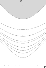
Figure 3: The expected joint spectrum of the operators $T,H$.

The states $v\in V_{p,\epsilon}$ with $(p,\epsilon)\in\operatorname{Hyp}_{i}$ are called elementary excitations. The numbers $m_{i}$ are called their masses.

The vector

$$\vec{m}=(m_{1},\ldots,m_{8})$$ (30)

is proportional to the Perron - Frobenius $v_{PF<}$ for $E_{8}$ from 4.10, whose normalized approximate value is

$$v_{PF<}=(1,1.62,1.99,2.40,2.96,3.22,3.89,4.78)$$ (31)

These low-lying excitations (hyperbolae) are observable: one may be able to see them

(a) in a computer simulation, or

(b) in a neutron scattering experiment.

6.2 Neutron scattering experiment

The paper Coldea reports the results of a magnetic neutron scattering experiment on cobalt niobate CoNb₂O₆, a material that can be pictured as a collection of parallel non-interacting one-dimensional chains of atoms. We depict such a chain as a straight line, parallel to the $z$-axis in our physical space $\mathbb{R}^{3}$ with coordinates $x,y,z$.

The sample, at low temperature $T<2.95$K (Kelvin), was subject to an external magnetic field with components $(h_{z},h_{z})$, with the $h_{x}$ at the critical value $h_{x}=h_{c}$, and with $h_{z}<<h_{c}$. The system may be described as the Ising chain with a nearly-critical Hamiltonian $H=H(J,h_{z}<<h_{c},h_{c})$ of the Eq. (27). The experiment Coldea may be interpreted with the help of the following (oversimplified) theoretical picture.

Consider a neutron scattering off the sample. If the incident neutron has energy $\epsilon$ and momentum $p$, and scatters off with energy $\epsilon^{\prime}$ and momentum $p^{\prime}$, the energy and momentum conservation laws imply that the differences, called energy and momentum transfers $\omega=\epsilon-\epsilon^{\prime},q=p-p^{\prime}$, are absorbed by the sample.

The energy transfer cannot be arbirtary. Suppose that, prior to scattering the neutron, the sample was in the ground state $v_{0}$; upon scattering the neutron, it undergoes a transition to a state that is a linear combination of the eight elementary excitations $v\in V_{p,\epsilon}$.

We will be interested in neutrons that scatter off with zero momentum transfer. The Zamolodchikov theory Z predicted, that the neutron scattering intensity $\mathcal{S}(0,\omega)$ should have peaks at $\omega=m_{a}$, ($a=1,...,8$) of the Eq. (31). At zero momentum transfer, a neutron scattering experiment would measure the proportion of neutrons that scattered off with the energies $m_{1},\ldots,m_{8}$: the resulting $\mathcal{S}(0,\omega)$ would look as in the schematic Fig. 4. Metaphorically speaking, the crystal would thus “sound” as a “chord” of eight “notes”: the eigenfrequencies $m_{i}$.

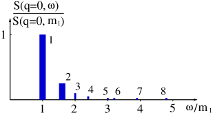
Figure 4: A sketch of the scattering intensity $\mathcal{S}(0,\omega)$ at zero momentum peaks relative to $\mathcal{S}(0,m_{1})$, against the $\omega/m_{1}$ ratio. The two leftmost peaks shown by thick lines correspond to the excitations with the masses $m_{1}$ and $m_{2}$, that were resolved in the experiment Coldea . The experimentally found mass ratio $m_{2}/m_{1}$ is consistent with $\frac{m_{2}}{m_{1}}=\frac{1+\sqrt{5}}{2}$, as per the expression for the $v_{Zam}(m)$ in the Subsection 4.10.

At the lowest temperatures, and in the immediate vicinity of $h_{x}=h_{c}$, the experiment Coldea succeeded to resolve the first two excitations, and to extract their masses $m_{1}$ and $m_{2}$. The mass ratio $m_{2}/m_{1}$ was found to be $\frac{m_{2}}{m_{1}}=1.6\pm 0.025$, consistent with $\frac{m_{2}}{m_{1}}=\frac{1+\sqrt{5}}{2}\approx 1.618$ of the expression for the $v_{Zam}(m)$ in the Subsection 4.10. In other words, the experimentalists were able to hear two of the eight notes of the Zamolodchikov $E_{8}$ chord.

A reader wishing to find out more about various facets of the story is invited to turn to the references Rajaraman ; Delfino ; Goss ; Borthwick .

- (1) V.Arnold, S.Gusein-Zade, A,Varchenko, Singularities of differentiable maps, vol. II, Monodrmomy and asymptotic of integrals.
- (2) N.Bourbaki, Groupes et algèbres de Lie, Chapitres IV - VI.
- (3) E.Brieskorn, Automorphic sets and braids and singularities, Contemp. Math. 78 (1988), 45 - 115.
- (4) B.Casselman, Essays on Coxeter groups. Coxeter elements in finite Coxeter groups, https://www.math.ubc.ca/ cass/research/pdf/Element.pdf
- (5) H.S.M.Coxeter, The product of the generators of a finite group generated by reflections, Duke Math. J. 18 (1951), 765 - 782.
- (6) P.Dorey, (a) Root systems and purely elastic -matrices, Nucl. Phys. B358 (1991), 654 - 676. (b) The exact -matrices of affine Toda field theories, Durham PhD thesis (1990).
- (7) A.Gabrielov, Intersection matrices for some singularities.Functional Analysis and Its Applications, July 1973, Volume 7, Issue 3, pp 182-193
- (8) A.Givental, Twisted Picard - Lefschetz formulas. Functional Analysis and Its Applications, January 1988, Volume 22, Issue 1, pp 10-18
- (9) K.Ireland, M.Rosen, A classical introduction to modern Number theory.
- (10) A.Knapp, Elliptic curves, Princeton University Press
- (11) B.Kostant, (a) The principal three-dimensional subgroup and the Betti numbers of a complex simple Lie group, Amer. J. Math. 81 (1959), 973 - 1032; see (6.5.1). (b) Experimental evidence for the occuring of in nature and Gosset circles, Selecta Math. 16 (2010), 419 - 438.
- (12) K.Lamotke, Die Homologie isolierter Singularitäten, Math. Z. 143 (1975), 27 - 44.
- (13) S.Lefschetz, L’analysis situs et la géométrie algébrique, Gauthier-Villars, 1950.
- (14) J.Milnor, Singular points of complex hypersurfaces.
- (15) A.V.Mikhailov, M.A.Olshanetsky, A.M.Perelomov, Two-dimensional generalized Toda lattice, Commun. Math. Phys. 79 (1981), 473 - 488.
- (16) M.Sebastiani, R.Thom, Un résultat sur la monodromie, Inv. Math. 13 (1971), 90 - 96.
- (17) J.-P.Serre, Cours d’arithmétique.
- (18) R.Steinberg, Finite subgroups of , Dynkin diagrams and affine Coxeter elements, Pacific J. Math. 118 (1985), 587 - 598.
- (19) A. B. Zamolodchikov, (a) Integrable field theory from Conformal field theory, in: Integrable Systems in Quantum Field Theory and Statistical Mechanics, Adv. Studies in Pure Math. 19 (1989), 641 - 674. (b) Integrals of motion and -matrix of the (scaled) Ising model with magnetic field, Int. J. Mod. Phys. A 4 (1989) 4235 - 4248.
- (20) R. Coldea, D. A. Tennant, E. M. Wheeler, E. Wawrzynska, D. Prabhakaran, M. Telling, K. Habicht, P. Smeibidl, K. Kiefer, Quantum Criticality in an Ising Chain: Experimental Evidence for Emergent Symmetry, Science 327 (2010), 177-180.
- (21) B. K. Chakrabarti, A. Dutta, P. Sen, Quantum Ising Phases and Transitions in Transverse Ising Models, Springer Lecture Notes in Physics, 1996.
- (22) R. Rajaraman, Solitons and instantons, North-Holland Publishing Company, 1989.
- (23) G. Delfino, Integrable field theory and critical phenomena: the Ising model in a magnetic field, J. Phys. A: Math. Gen. 37 (2004) R45 - R78.
- (24) B. Goss Levi, A complex symmetry arises at a spin chain’s quantum critical point, Physics Today 63 (3), 13 (2010); doi: 10.1063/1.3366227 View online: http://dx.doi.org/10.1063/1.3366227 .
- (25) D. Borthwick, S. Garibaldi, Did a 1-Dimensional Magnet Detect a 248-Dimensional Lie Algebra?, AMS Notices 58 (2011), 1055 - 1065.