Partitioning Graph Drawings
and Triangulated Simple Polygons
into Greedily Routable Regions

Abstract

A greedily routable region (GRR) is a closed subset of $\mathbb{R}^{2}$, in which any destination point can be reached from any starting point by always moving in the direction with maximum reduction of the distance to the destination in each point of the path. Recently, Tan and Kermarrec proposed a geographic routing protocol for dense wireless sensor networks based on decomposing the network area into a small number of interior-disjoint GRRs. They showed that minimum decomposition is -hard for polygonal regions with holes.

We consider minimum GRR decomposition for plane straight-line drawings of graphs. Here, GRRs coincide with self-approaching drawings of trees, a drawing style which has become a popular research topic in graph drawing. We show that minimum decomposition is still -hard for graphs with cycles and even for trees, but can be solved optimally for trees in polynomial time, if we allow only certain types of GRR contacts. Additionally, we give a 2-approximation for simple polygons, if a given triangulation has to be respected.

Keywords:

Greedy region decomposition; increasing-chord drawings; decomposing graph drawings; greedy routing in wireless sensor networks.

1 Introduction

Geographic or geometric routing is a routing approach for wireless sensor networks that became popular recently. It uses geographic coordinates of sensor nodes to route messages between them. One simple routing strategy is greedy routing. Upon receipt of a message, a node tries to forward it to a neighbor node that is closer to the destination than itself. However, delivery cannot be guaranteed, since a message may get stuck in a local minimum or void. Another local routing strategy is compass routing. It forwards the message to a neighbor, such that the direction from the node to this neighbor is closest to the direction from the node to the destination. Kranakis et al. [15] showed that compass routing can produce loops even in plane triangulations. They also showed that compass routing is always successful on Delaunay triangulations. More advanced geometric routing protocols employ strategies like face routing [2] and related techniques based on planar graphs to get out of local minima; see [17, 5] for an overview.

An alternative approach is to decompose the network into components such that in each of them greedy routing is likely to perform well [10, 21, 23]. A global data structure of preferably small size is used to store interconnectivity between components. One such network decomposition approach has been recently proposed by Tan and Kermarrec [22]. They assume that global connectivity irregularities, i.e, large holes in the network and the network boundary, are the main source of local minima in which greedy routing between a pair of sensor nodes might get stuck. They note that in practical sensor networks, local connectivity irregularity normally has low impact on the cost of routing and the quality of the resulting paths, since the local minima in this context can be overcome by simple and light-weight techniques; see [22] for a list of such strategies. With this reasoning, Tan and Kermarrec model the network as a polygonal region with obstacles or holes inside it and consider greedy routing inside this continuous domain. Local minima now only appear on the boundaries of the polygonal region. In this work, we use the same model.

Tan and Kermarrec [22] try to partition this region into a minimum number of polygons, in which greedy routing works between any pair of points. They call such components greedily routable regions (GRRs). For intercomponent routing, region adjacencies are stored in a graph. The protocol is able to guarantee finding paths of bounded stretch, i.e., the length of such a path exceeds the distance between its endpoints only by a constant factor.

For routing in the underlying network of sensor nodes corresponding to discrete points inside the polygonal region, greedy routing is used if the source and the destination nodes are in the same component, and existing techniques are used to overcome local minima. For inter-component routing, each node stores a neighbor on a shortest path to each component. This path is used to get to the component of the destination, and then intra-component routing is used.

Tan and Kermarrec [22] emphasize the importance for the nodes to store as small routing tables as possible and note that the number of network components in a decomposition directly reflects the number of nonlocal routing states of a node. This number determines the size of the node’s routing table. Therefore, the goal is to partition the network into a minimum number of GRRs. In this work, we focus on the problem of partitioning a polygonal region or a graph drawing (for which we extend the notion of a GRR) into a minimum number of GRRs. For a detailed description of an actual routing protocol based on GRR decompositions, see the original work of Tan and Kermarrec [22].

The authors prove that partitioning a polygon with holes into a minimum number of regions is -hard and they propose a simple heuristic. Its solution may strongly deviate from the optimum even for very simple polygons; see Fig. 2a.

Some real-world instances from the work of Tan and Kermarrec [22, Fig. 17] are networks of sensor nodes distributed on roads of a city. The resulting polygonal regions are very narrow and strongly resemble plane straight-line graph drawings. Therefore, considering plane straight-line graph drawings in addition to polygonal regions is a natural adjustment of the minimum GRR partition problem.

In this paper, we approach the problem of finding minimum or approximately minimum GRR decompositions by first considering the special case of partitioning drawings of graphs, which can be interpreted as very thin polygonal regions. We notice that in this scenario, GRRs coincide with increasing-chord drawings of trees as studied by Alamdari et al. [1].

A self-approaching curve is a curve, where for any point $t^{\prime}$ on the curve, the Euclidean distance to $t^{\prime}$ decreases continuously while traversing the curve from the start to $t^{\prime}$ [12]. An increasing-chord curve is a curve that is self-approaching in both directions. The name is motivated by their equivalent characterization as those curves, where for any four points $a,b,c,d$ in this order along the curve, $|bc|\leq|ad|$, where $|pq|$ denotes the Euclidean distance from point $p$ to point $q$.

A graph drawing is self-approaching or increasing-chord if every pair of vertices is joined by a self-approaching or increasing-chord path, respectively. The study of self-approaching and increasing-chord graph drawings was initiated by Alamdari et al. [1]. They studied the problem of recognizing whether a given graph drawing is self-approaching and gave a complete characterization of trees admitting self-approaching drawings. In our own previous work [19], we studied self-approaching and increasing-chord drawings of triangulations and 3-connected planar graphs. Furthermore, the problem of connecting given points to form an increasing-chord drawing has been investigated [1, 9].

Contributions.

First, we show that partitioning a plane graph drawing into a minimum number of increasing-chord components is -hard. This extends the result of Tan and Kermarrec [22] for polygonal regions with holes to plane straight-line graph drawings. Next, we consider plane drawings of trees. We show that the problem remains -hard even for trees, if arbitrary types of GRR contacts are allowed. For a restriction on the types of GRR contacts, we show how to model the decomposition problem using Minimum Multicut, which provides a polynomial-time 2-approximation. We then solve the partitioning problem for trees and restricted GRR contacts optimally in polynomial time using dynamic programming. Finally, we use the insights gained for decomposing graphs and apply them to the problem of minimally decomposing simple triangulated polygons into GRRs. We provide a polynomial-time 2-approximation for decompositions that are formed along chords of the triangulation.

2 Preliminaries

In the following, let $\mathcal{P}$ be a polygonal region, and let $\partial\mathcal{P}$ denote its boundary. For $p\in\mathcal{P}$, let $V(p)$ denote the visibility region of $p$, i.e., the set of points $q\in\mathcal{P}$ such that the line segment $pq$ lies inside $\mathcal{P}$. For directions $\vv{d_{1}}$ and $\vv{d_{2}}$, let $\angle(\vv{d_{1}},\vv{d_{2}})\leq 180^{\circ}$ denote the angle between them. For points $p,q$, $p\neq q$, let $\textnormal{ray}(p,q)$ denote the ray with origin $p$ and direction $\vv{pq}$.

Definition 1.

For an $s$-$t$-path $\rho$ and a point $p\neq t$ on $\rho$, we define the forward tangent on $\rho$ in $p$ as the direction $\vv{d}=\lim_{\varepsilon\rightarrow 0}\{\vv{pq}\mid q\textnormal{ succeeds }p\textnormal{ on }\rho\textnormal{, and }|pq|=\varepsilon\}$.

Next, we formally define paths resulting from greedy routing inside $\mathcal{P}$. We call such paths greedy. Note that this definition of greediness is different from the one used in the context of greedy embeddings of graphs [20].

Definition 2.

For points $s,t\in\mathcal{P}$, an $s$-$t$-path $\rho$ is greedy if the distance to $t$ strictly decreases along $\rho$ and if for every point $s^{\prime}\neq t$ on $\rho$, the forward tangent $\vv{d}$ on $\rho$ in $s^{\prime}$ has the minimum angle with $\vv{s^{\prime}t}$ among all vectors $\vv{s^{\prime}q}$ for any $q\in V(s^{\prime})\setminus\{s^{\prime}\}$.

(a)

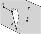
(b)

Figure 1: LABEL:sub@fig:greedy-path The thick $s$-$t$-path inside the polygonal region $\mathcal{P}$ (grey) is greedy. LABEL:sub@fig:greedy-path-alg If $t$ is not visible, a greedy path must trace an edge until the endpoint. If it is not possible, a local minimum must exist.

A greedy path is shown in Fig. 1a. Note that such paths are polylines. The way greedy paths are defined resembles compass routing [15].

2.1 Greedily Routable Regions.

Greedily Routable Regions were introduced by Tan and Kermarrec [22] as follows.

Definition 3 ( [22]).

A polygonal region $\mathcal{P}$ is a greedily routable region (GRR), if for any two points $s,t\in\mathcal{P}$, $s\neq t$, point $s$ can always move along a straight-line segment within $\mathcal{P}$ to some point $s^{\prime}$ such that $|s^{\prime}t|<|st|$.

Next we show that $\mathcal{P}$ is a GRR if and only if every pair of points in $\mathcal{P}$ is connected by a greedy path. Therefore, Definition 3 is equivalent to the one used in the abstract. We shall show that the following procedure produces a greedy path inside a GRR.

1 Set $p=s$.

2If $t$ is visible from $p$, move $p$ to $t$ and finish the procedure.

3Move $p$ to the first intersection of $pt$ and $\partial\mathcal{P}$. (Note that $p$ itself may be the first intersection.)

4If $p$ is in the interior of a boundary edge $v_{1}v_{2}$, consider the angle between $\vv{pv_{i}}$ and $\vv{pt}$, $i=1,2$. Let $v_{i}$ be the vertex minimizing $\angle(\vv{pv_{i}},\vv{pt})$, $i=1,2$ (break ties arbitrarily). If $v_{i}$ is the closest point to $t$ on the segment $pv_{i}$, move $p$ to $v_{i}$ and return to Step 2, otherwise, return failure.

5If $p$ coincides with the vertex $v_{2}$ incident to boundary edges $v_{1}v_{2}$ and $v_{2}v_{3}$, consider the angle between $\vv{pv_{i}}$ and $\vv{pt}$, $i=1,3$. Let $v_{i}$ be the vertex minimizing $\angle(\vv{pv_{i}},\vv{pt})$, $i=1,3$ (break ties arbitrarily). Again, if $v_{i}$ is the closest point to $t$ on the segment $pv_{i}$, move $p$ to $v_{i}$ and return to Step 2, otherwise, return failure.

Procedure 1 Constructing a greedy $s$-$t$-path inside a GRR.

Lemma 1.

A polygonal region $\mathcal{P}$ is a GRR if and only if for every $s,t\in\mathcal{P}$ there exists a greedy $s$-$t$-path $\rho\subseteq\mathcal{P}$. Procedure 1 produces such a greedy path.

Proof.

First, consider $s,t\in\mathcal{P}$ connected by a greedy $s$-$t$-path $\rho$. Then $s,t$ satisfy the condition in Definition 3 using the endpoint $s^{\prime}$ of the first segment $ss^{\prime}$ of $\rho$.

Conversely, let $\mathcal{P}$ be a GRR. Let $s,t$ be two distinct points in $\mathcal{P}$, and consider a path $\rho$ constructed by moving a point $p$ from $s$ to $t$ according to Procedure 1. We consider the segments of $\rho$ iteratively and show that each of them would be taken by a greedy path. Since $\mathcal{P}$ is a GRR, every point $p\in\mathcal{P}$ can get closer to $t$ by a linear movement. If all points on $\textnormal{ray}(p,t)$ sufficiently close to $p$ are in $\mathcal{P}$, a greedy path would move along $\textnormal{ray}(p,t)$, until it hits $\partial\mathcal{P}$. This shows that Step 3 of the procedure traces a greedy path.

Assume all points on $\textnormal{ray}(p,t)$ sufficiently close to $p$ are not in $\mathcal{P}$. Then, $p$ is on $\partial\mathcal{P}$. Let $\vv{d_{1}}$ and $\vv{d_{2}}$ be the two tangents in $p$ to the paths that start at $p$ and go along $\partial\mathcal{P}$. Let $\Lambda$ be the cone of directions spanned by $\vv{d_{1}}$ and $\vv{d_{2}}$, such that $\vv{pt}\notin\Lambda$. Then, $\Lambda$ contains the directions of all possible straight-line movements from $p$. By Definition 3, for some direction $\vv{d}\in\Lambda$, we have $\angle(\vv{pt},\vv{d})<90^{\circ}$. But then, $\min_{i=1,2}\angle(\vv{pt},\vv{d_{i}})\leq\angle(\vv{pt},\vv{d})<90^{\circ}$. Therefore, a greedy path would continue in the direction $\vv{d_{i}}$, as does $\rho$. Let $v_{i}$ be the endpoint of the edge containing $p$, such that $\vv{pv_{i}}=\vv{d_{i}}$. Therefore, $\angle tpv_{i}<90^{\circ}$. We must show that a greedy path is traced if $p$ follows $\vv{d_{i}}$ until $v_{i}$. We have $\angle pv_{i}t\geq 90^{\circ}$. Otherwise, the projection point $x$ of $t$ on the line through $pv_{i}$ lies in the interior of the segment $pv_{i}$ and is a local minimum with respect to the distance to $t$, which is not possible in a GRR; see Fig. 1b. Therefore, when $p$ moves in the direction $\vv{d_{i}}$ towards $v_{i}$, its distance to $t$ decreases continuously, and the forward tangent always has the minimum possible angle with respect to the direction towards $t$. This shows that Steps 4 and 5 of the procedure trace a greedy path and never return failure.

It follows that, when moving along $\rho$, point $p$ either moves directly to $t$ or slides along a boundary edge until it reaches one of the endpoints. Therefore, point $p$ never reenters an edge and must finally reach $t$. The forward tangent on $\rho$ always satisfies the condition of Definition 2, therefore, $\rho$ is a greedy $s$-$t$-path.

∎

A decomposition of a polygonal region $\mathcal{P}$ is a partition of $\mathcal{P}$ into polygonal regions $\mathcal{P}_{i}$ with no holes, $i=1,\dots,k$, such that $\bigcup_{i=1}^{k}\mathcal{P}_{i}=\mathcal{P}$ and no $\mathcal{P}_{i}$, $\mathcal{P}_{j}$ with $i\neq j$ share an interior point. Recall that GRRs have no holes. A decomposition of $\mathcal{P}$ is a GRR decomposition if each component $\mathcal{P}_{i}$ is a GRR. We shall use the terms GRR decomposition and GRR partition interchangeably. Using the concept of a conflict relationship between edges of a polygonal region (see Fig. 2b), Tan and Kermarrec give a convenient characterization of GRRs.

Definition 4 (Normal ray).

Let $\mathcal{P}$ be a polygonal region, $e=uv$ a boundary edge and $p$ an interior point of $uv$. Let $\textnormal{ray}_{uv}(p)$ denote the ray with origin in $p$ orthogonal to $uv$, such that all points on this ray sufficiently close to $p$ are not in the interior of $\mathcal{P}$.

(a)

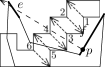
(b)

Figure 2: LABEL:sub@fig:heuristic-bad The heuristic in [22] splits a non-greedy region by a bisector at a maximum reflex angle. If the splits are chosen in order of their index, seven regions are created, although two is minimum (split only at 6). LABEL:sub@fig:conflict Normal ray $\textnormal{ray}_{f}(p)$ and a pair of conflicting edges $e$, $f$.

We restate the definition of conflicting edges from [22].

Definition 5 (Conflicting edges of a polygonal region).

Let $e$ and $f$ be two edges of a polygonal region $\mathcal{P}$. If for some point $p$ in the interior of $e$, $\textnormal{ray}_{e}(p)$ intersects $f$, then $e$ conflicts with $f$.

A polygonal region is a GRR if and only if it has no pair of conflicting edges; [22, Theorem 1]. Furthermore, GRRs are known to have no holes.

Now consider a plane straight-line drawing $\Gamma$ of a graph $G=(V,E)$. We identify the edges of $G$ with the corresponding line segments of $\Gamma$ and the vertices of $G$ with the corresponding points. Plane straight-line drawings can be considered as infinitely thin polygonal regions. The routing happens along the edges of $\Gamma$, and we define GRRs for graph drawings as follows.

Definition 6 (GRRs for plane straight-line drawings).

A plane straight-line graph drawing $\Gamma$ is a GRR if for any two points $s\neq t$ on $\Gamma$ there exists a point $s^{\prime}$ on an edge that also contains $s$, such that $|s^{\prime}t|<|st|$.

Note that for an interior point $p$ of an edge $e$ of $\Gamma$ there exist two normal rays at $p$ with opposite directions. Let $\textnormal{n}_{e}(p)$ denote the normal line to $e$ at $p$. We define conflicting edges of $\Gamma$ as follows.

Definition 7 (Conflicting edges of a plane straight-line drawing).

Let $e$ and $f$ be two edges of a plane straight-line drawing $\Gamma$. If for some point $p$ in the interior of $e$, $\textnormal{n}_{e}(p)$ intersects $f$, then $e$ conflicts with $f$.

Assume $\textnormal{n}_{e}(s)$ for an interior point $s$ on an edge $e$ of $\Gamma$ crosses another edge $f$ in point $t$. Then, any movement along $e$ starting from $s$ increases the distance to $t$. We call such edges conflicting. It is easy to see that $\Gamma$ is a GRR if it contains no pair of conflicting edges. Obviously, such a drawing $\Gamma$ contains no cycles. In fact, a straight-line drawing of a tree is increasing-chord if and only if it has no conflicting edges [1], which implies the following lemma.

Lemma 2.

The following two properties are equivalent for a straight-line drawing $\Gamma$ to be a GRR.

1. $\Gamma$ is connected and has no conflicting edges;

2. $\Gamma$ is an increasing-chord drawing of a tree.

Since every individual edge in a straight-line drawing is a GRR, the following observation can be made on the worst-case size of a minimum GRR partition.

Observation 1.

A plane straight-line drawing $\Gamma$ of graph $G=(V,E)$, $|E|=m$, has a GRR decomposition of size $m$.

Therefore, if $G$ is a tree, the drawing $\Gamma$ has a GRR partition of size $n-1$ for $n=|V|$.

2.2 Splitting graph drawings at non-vertices.

Note that in a GRR partition of a plane straight-line drawing $\Gamma$ of a graph $G=(V,E)$, an edge $e\in E$ does not necessarily lie in one GRR. Pieces of the same edge can be part of different GRRs. Allowing splitting edges at intermediate points might result in smaller GRR partitions; see Fig. 3. In this section, we discuss splitting $\Gamma$ at non-vertices. We will show that there are only a discrete set of $O(n^{2})$ points where we might need to split edges.

(a)

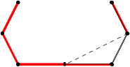
(b)

Figure 3: Splitting at non-vertices results in a smaller partition. LABEL:sub@fig:split-nonvertex:1 No pair of the thick red edges can be in the same GRR. Therefore, if no edge splits are allowed, every GRR partition has size at least 3. LABEL:sub@fig:split-nonvertex:2 Splitting the longest edge results in a GRR partition of size 2.

Definition 8 (Subdivided drawing $\Gamma_{s}$).

Let $\Gamma_{s}$ be the drawing created by subdividing edges of $\Gamma$ as follows. For every pair of original edges $u_{1}u_{2},u_{3}u_{4}\in E$, let $\ell_{i}$ be the normal to $u_{1}u_{2}$ at $u_{i}$, $i=1,2$. If $\ell_{i}$ intersects $u_{3}u_{4}$, we subdivide $u_{3}u_{4}$ at the intersection.

Since we consider only the original edges of $\Gamma$, the subdivision $\Gamma_{s}$ has $O(n^{2})$ vertices.

Lemma 3.

Any GRR decomposition of $\Gamma$ with potential edge splits can be transformed into a GRR decomposition of $\Gamma_{s}$ in which no edge of $\Gamma_{s}$ is split, such that the size of the decomposition does not increase.

Proof.

Consider edge $uv$ of the subdivision $\Gamma_{s}$, a point $x$ in its interior and assume an increasing-chord component $C$ (green in Fig. 4) contains $vx$, but not $ux$. We claim that we can reassign $ux$ to $C$. Note that iterative application of this claim implies the lemma.

(a)

Figure 4: Proof of Lemma 3. Segment $ux$ can be added to the thick green GRR $C$, such that the entire edge $uv$ of $\Gamma_{s}$ is in one GRR.

For points $p,q\in\mathbb{R}^{2},p\neq q$, let $l_{pq}^{+}$ denote the halfplane not containing $p$ bounded by the line through $q$ orthogonal to the segment $pq$. Note that if segment $pq$ is on the path from vertex $p$ to vertex $r$ in an increasing-chord tree drawing then $r\in l_{pq}^{+}$ [1].

Let $u_{2}v_{2}$ be an original edge of $\Gamma$ such that $v_{2}$ is in $C$, as well as a subsegment $yv_{2}$ of $u_{2}v_{2}$ with a non-zero length containing $v_{2}$. Since segment $yv_{2}$ is on the $y$-$v$-path in $C$, the halfplane $l_{u_{2}v_{2}}^{+}=l_{yv_{2}}^{+}$ contains $v$, and its boundary does not cross $uv$ by the construction of $\Gamma_{s}$. Thus, $l_{u_{2}v_{2}}^{+}$ contains $uv$. In this way, we have shown that no normal ray of an edge of $C$ crosses $uv$.

Furthermore, $l_{uv}^{+}=l_{xv}^{+}$. Since $C-xv$ lies entirely in $l_{xv}^{+}=l_{uv}^{+}$, this shows that no normal of $uv$ crosses another edge of $C$. It follows that the union of $C$ and $ux$ contains no conflicting edges and, therefore, is increasing-chord by Lemma 2.

Finally, removing $ux$ from the component $C^{\prime}$ containing it doesn’t disconnect them, since no edge or edge part is attached to $x$ (or an interior point of $ux$). Since $C^{\prime}-ux$ is connected and $C^{\prime}$ is a GRR, $C^{\prime}-ux$ is also a GRR. ∎

2.3 Types of GRR contacts in plane straight-line graph drawings

We distinguish the types of contacts that two GRRs can have in a GRR partition of a plane straight-line graph drawing.

Definition 9 (Proper, non-crossing and crossing contacts).

Consider two drawings $\Gamma_{1}$, $\Gamma_{2}$ of trees with the only common point $p$.

1. $\Gamma_{1}$ and $\Gamma_{2}$ have a proper contact if $p$ is a leaf in at least one of them.

2. $\Gamma_{1}$ and $\Gamma_{2}$ have a non-crossing contact if in the clockwise ordering of edges of $\Gamma_{1}$ and $\Gamma_{2}$ incident to $p$, all edges of $\Gamma_{1}$ (and, thus, also of $\Gamma_{2}$) appear consecutively.

3. $\Gamma_{1}$ and $\Gamma_{2}$ are crossing or have a crossing contact if in the clockwise ordering of edges of $\Gamma_{1}$ and $\Gamma_{2}$ incident to $p$, edges of $\Gamma_{1}$ (and, thus, also of $\Gamma_{2}$) appear non-consecutively.

The first part of Definition 9 allows GRRs to only have contacts as shown in Fig. 5a and forbids contacts as shown in Fig. 5b, 5c. The second part allows contacts as those in Fig. 5b, but forbids the contacts in Fig. 5c.

Note that a contact of two trees $\Gamma_{1},\Gamma_{2}$ with a single common point $p$ is either crossing or non-crossing. Moreover, if the contact of $\Gamma_{1}$ and $\Gamma_{2}$ is proper, then it is necessarily non-crossing, since for a proper contact, $\Gamma_{1}$ or $\Gamma_{2}$ has only one edge incident to $p$, therefore, all edges of $\Gamma_{1}$ and of $\Gamma_{2}$ appear consecutively around $p$.

We shall show that for trees, restricting ourselves to GRR decompositions with only non-crossing contacts makes the otherwise -complete problem of finding a minimum GRR partition solvable in polynomial time.

(a)

(b)

(c)

Figure 5: LABEL:sub@fig:trees:proper Proper GRR contact; LABEL:sub@fig:trees:non-proper:non-crossing non-crossing contact which is not proper and LABEL:sub@fig:trees:non-proper:crossing crossing contact.

3 NP-completeness for graphs with cycles

We show that finding a minimum decomposition of a plane straight-line drawing $\Gamma$ into increasing-chord trees is -hard. This extends the -hardness result by Tan and Kermarrec [22] for minimum GRR decompositions of polygonal regions with holes to plane straight-line drawings.

Note that in the graph drawings used for our proof, all GRRs will have proper contacts; see Definition 9. Moreover, the graph drawings can be turned into thin polygonal regions in a natural way by making them slightly “thicker”, and the proof can be reused as another proof for the -hardness result in [22].

Both our -hardness proof and the proof in [22] are reductions from the -complete problem Planar 3SAT [16]. Recall that a Boolean 3SAT formula $\varphi$ is called planar, if the corresponding variable clause graph $G_{\varphi}$ having a vertex for each variable and for each clause and an edge for each occurrence of a variable (or its negation) in a clause is a planar graph. In fact, $G_{\varphi}$ can be drawn in the plane such that all variable vertices are aligned on a vertical line and all clause vertices lie either to the left or to the right of this line and connect to the variables via E- or $\exists$-shapes [14]; see Fig. 6.

Figure 6: An orthogonal graph drawing of the variable-clause graph $G_{\varphi}$ for a planar 3SAT formula $\phi=(w\vee x\vee z)\wedge~{}(\bar{x}\vee y\vee\bar{z})\wedge~{}(\bar{w}\vee\bar{x}\vee\bar{z})$.

The basic idea of the gadget proof is as follows. Using a number of building blocks, or gadgets, we construct a plane straight-line drawing $\Gamma_{\varphi}$, whose geometry mimics the variable-clause graph $G_{\varphi}$ drawn as described above. We construct $\Gamma_{\varphi}$ in a way such that its minimum GRR decompositions are in correspondence with the truth assignments of the Planar 3SAT formula $\varphi$.

The variable gadgets in [22] are cycles formed by T-shaped polygons which can be made arbitrarily thin. Thus, in the case of plane straight-line drawings we can use very similar variable gadgets (see Fig. 7). The clause gadgets in [22], however, are squares, at which three variable cycles meet. This construction cannot be adapted for straight-line plane drawings, and we have to construct a significantly different clause gadget; see Fig. 9.

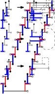
(a)

(b)

(c)

Figure 7: Variable gadget and the two possibilities to pair vertical and horizontal segments to make GRRs: LABEL:sub@fig:cycles:var-true true variable state: $\top$-shapes and $\bot$-shapes; LABEL:sub@fig:cycles:var-false false variable state: $\dashv$-shapes and $\vdash$-shapes. LABEL:sub@fig:cycles:var-arm-stubs Extending the variable gadgets to create the upper, middle and lower arm gadgets by substituting T-shapes of the variable gadget.

(a)

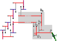
(b)

Figure 8: Variable gadget with a right upper positive arm (shaded region). LABEL:sub@fig:cycles:arm-pos-true true and LABEL:sub@fig:cycles:arm-pos-false false states.

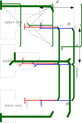
(a)

(b)

Figure 9: Clause gadget (thick green). (a) true and (b) false state of the involved literals.

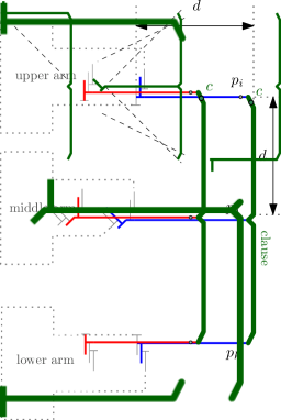
(a)

(b)

Figure 10: Merging the clause gadget with GRRs from the arm loops. (a) None of the three components is a GRR. (b)  All three components are GRRs; see the dashed normals.

We define a variable gadget as a cycle of alternating vertical and horizontal segments. The tip of each segment touches an interior point of the next segment. We can join pairs of consecutive segments into a GRR by assigning each vertical segment either to the next or to the previous horizontal segment on the cycle. In this way, the variable loop is partitioned either in $\top$-shapes and $\bot$-shapes or in $\dashv$-shapes and $\vdash$-shapes; see Fig. 7.

Consider a variable gadget consisting of $k$ T-shapes as shown in Fig. 7. On each T-shape we place one black and one white point as shown in the figure. The points are placed in such a way that neither two black points nor two white points can be in one increasing-chord component. Thus, a minimum GRR decomposition of a variable gadget contains at least $k$ components. If it contains exactly $k$ components, then each component must contain one black and one white point, and there are exactly two possibilities. Each black point has exactly two white points it can share a GRR with, and once one pairing is picked, it fixes all the remaining pairings. The corresponding possibilities are shown in Fig. 7a and 7b and will be used to encode the values true and false, respectively. For the pairing of the black and white points corresponding to the true state, the variable loop can be partitioned in $\top$-shapes and $\bot$-shapes, and for the pairing corresponding to the false state, it can be partitioned in $\dashv$-shapes and $\vdash$-shapes.

To pass the truth assignment of a variable to a clause it is part of, we use arm gadgets. Arm gadgets are extensions of the variable gadget. To add an arm gadget to the variable, we substitute several $\top$- or $\bot$-shapes from the variable loop by a more complicated structure. Fig. 7c shows such extensions for all arm types pointing to the right, the other case is symmetric. In this way, for a variable, we can create as many arms as necessary. Each variable loop will have one arm extension for each occurrence of the corresponding variable in a clause in $\varphi$. The working principle for the arm gadgets is the same as for the variable gadgets. The drawing created by the variable cycle and the arm extensions (the variable-arm loop) will once again contain distinguished black and white points, such that only one black and one white point can be in a GRR. However, for variable-arm loops, the cycles formed by segments of varying orientation are more complicated than the loop in Fig. 7. For example, for some arm types we use segments of slopes $\pm 1$ in addition to vertical and horizontal segments.

In total twelve variations of the arm gadget will be used, depending on the position of the literal in the clause, the position of the clause, and whether the literal is negated or not. Since in $G_{\varphi}$ each clause $c$ connects to three variables, we denote these variables or literals as the upper, middle, and lower variables of $c$ depending on the order of the three edges incident to $c$ in the one-bend orthogonal drawing of $G_{\varphi}$ used by Knuth and Raghunathan [14]; see Fig. 6. Similarly, an arm of $c$ is called an upper, middle, or lower arm if it belongs to a literal of the same type in $c$. An arm is called a right (resp. left) arm if it belongs to a clause that lies to the right (resp. to the left) of the vertical variable line. Finally, an arm of $c$ is positive if the corresponding literal is positive in $c$ and it is negative otherwise.

The basic principle of operation of any arm gadget is the same; as an example consider the right upper positive arm in Fig. 8. Figures 11, 12, 13 and the proof of Property 2 cover the remaining arm types.

The positive and the negative arms are differentiated by an additional structure that switches the pairing of the black and white points close to the part of the arm that touches the clause gadget; for example, compare Fig. 8b and 13a. By this inversion, for a fixed truth assignment of the variable, the $\top$- and $\bot$-shapes next to the clause are turned into $\vdash$- and $\dashv$-shapes, and vice versa. In this way, the inverted truth assignment of the corresponding variable is passed to the clause.

Note that each arm can be arbitrarily extended both horizontally and vertically to reach the required point of its clause gadget. We select again black and white points (also called distinguished points) on the line segments of the arm gadget.

The clause gadget (the thickest green polyline in Fig. 9, partly drawn in Fig. 8) is a polyline which consists of six segments. The first segment has slope 2, the second is vertical, the third has slope $-1$, the fourth has slope 1, the fifth is vertical, and the sixth has slope $-2$. Each clause gadget connects to the long horizontal segments of the arms of three variable gadgets. The three connecting points of the clause gadget are the start and end of the polyline as well as its center, which is the common point of the two segments with slopes $\pm 1$.

We shall prove the following property which is crucial for our construction.

Property 1.

1. Consider a drawing $\Gamma_{i}$ of a variable gadget together with all of its arms. Then, neither two black nor two white points on $\Gamma_{i}$ can be in one GRR. In a minimum GRR decomposition of $\Gamma_{i}$, each component has one black and one white point, and exactly two such pairings of points are possible, one for each truth assignment.

2. Consider two such drawings $\Gamma_{i}$, $\Gamma_{j}$ for two different variables. Then, no distinguished point of $\Gamma_{i}$ can be in the same GRR as a distinguished point of $\Gamma_{j}$.

Proof.

Part (1) of Property 1 extends the same property that we already showed for variable gadgets without arms to the case including all arms. It is an immediate consequence of the way we constructed the arm gadgets and placed the distinguished points; see Figures 8, 11, 12, 13.

Part (2) follows from the way the arms are connected by a clause, i.e., in Fig. 9 no pair of points from $p_{i}$, $p_{j}$, $p_{k}$ can be in the same GRR, since the three points lie on three horizontal segments and are vertically collinear. ∎

The clause gadget is connected to the arm by a horizontal segment with a distinguished point $p$ on its end, which is either black or white depending on the arm type. Each clause has one special point $c$ chosen as shown in Fig. 9.

We show that $c$ and $p$ can be in the same GRR in a minimum GRR decomposition if and only if the variable gadget containing $p$ is in the state that satisfies the clause.

Property 2.

1. In a minimum GRR decomposition, the special point $c$ of a clause gadget can share a GRR with a black or white point of an arm gadget if and only if the corresponding literal is in the true state.

2. If a variable assignment satisfies a clause, then its entire clause gadget can be contained in a GRR of an arm corresponding to a true literal.

Proof.

For each arm gadget we select a special red point $q$; see Fig. 8. Point $q$ is neither white nor black. By Property 1, in a minimum GRR decomposition, point $q$ must be in a GRR together with one black and one white point.

For the various arm types, if points $q$ and $p$ are in the same GRR, we shall show that this GRR cannot contain the entire clause gadget and, in particular, cannot contain point $c$. This is illustrated in Fig. 10a.

Furthermore, we shall show that if the literal is in the true state, then points $p$ and $q$ are in different GRRs, and the GRR containing $p$ can be merged with the entire clause gadget, including $c$. For example, in Fig. 9a, each variable is in a state that satisfies the clause. The lengths of the thick segments are chosen such that each thick blue component can be merged with the clause gadget (thickest green) into a single GRR, as shown in Fig. 10b.

$i)$ We first show the lemma for a positive right upper arm. We use the notation from Fig. 8 to refer to the distinguished points. In the true state of the variable (see Fig. 8a), points $w_{1}$, $b_{1}$ and $q$ are in the same GRR. Points $b_{2}$ and $p$ are in another GRR (e.g., the thickest green one in Fig. 8) which can contain the distinguished point $c$ of the clause.

In the false state of the variable (see Fig. 8b), the points $b_{1}$ and $p$ are in the same GRR. Moreover, point $q$ can share a GRR with exactly one point from $b_{1}$, $b_{2}$ or $b_{3}$. But if $q$ were with $b_{2}$ or $b_{3}$, then $b_{1}$ would be disconnected from any white point, a contradiction to the minimality of the decomposition. Thus, points $q$, $b_{1}$ and $p$ are in the same GRR, which cannot contain a point of the clause.

(a)

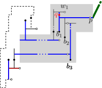
(b)

Figure 11: Right lower negative arm gadget. LABEL:sub@fig:cycles:arm-neg-false-2 false and LABEL:sub@fig:cycles:arm-neg-true-2 true variable state. Thin dashed lines indicate that the variable-arm loop continues.

$ii)$ We now show the lemma for a negative right lower arm. We use the notation from Fig. 11. In the false state of the variable (which corresponds to the true state of the considered literal), points $w_{1}$, $b_{1}$ and $q$ are in the same GRR; see Fig. 11a Points $b_{2}$ and $p$ are in another GRR (e.g., the very thick green one in Fig. 8) which can contain the entire clause; see the lower arm in Fig. 9 and the corresponding merged component in Fig. 10b.

Now consider a true state of the variable; see Fig. 11b. Point $q$ shares a GRR with exactly one point from $b_{1}$, $b_{2}$ or $b_{3}$. If $q$ is with $b_{2}$ or $b_{3}$, then $b_{1}$ is disconnected from any white point, a contradiction to the minimality of the decomposition. Thus, points $q$, $b_{1}$ and $p$ are in the same GRR, which cannot contain a point of the clause.

$iii)$ Next, consider a positive right middle arm; see Fig. 12. We identify points $p$ and $b_{1}$. Point $b_{1}$ is either with $w_{0}$ (true state of the variable) or $w_{1}$ (false state of the variable).

In the true state, points $b_{1}$ and $w_{0}$ are in one GRR, which cannot contain $q$. This GRR can be merged with the clause gadget; see Fig. 12a, 9 and 10b.

In the false state, points $b_{1}$, $w_{1}$ and $q$ are in one GRR, which cannot contain point $c$ of the clause.

(a)

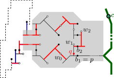
(b)

Figure 12: Right positive middle arm gadget. LABEL:sub@fig:cycles:arm-neg-true-3 true and LABEL:sub@fig:cycles:arm-neg-false-3 false variable state.

$iv)$ To construct the negative right upper arm, the positive right lower arm and the negative right middle arm, we invert the arm gadgets constructed before. The inverted gadgets are shown in Fig. 13. The proofs are analogous to the respective non-inverted cases.

$v)$ The left arms are constructed by mirroring. ∎

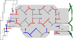
(a)

(b)

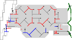
(c)

Figure 13: The remaining three right arms in the satisfying variable state. LABEL:sub@fig:cycles:arm-inv-1 negative right upper arm, LABEL:sub@fig:cycles:arm-inv-2 the positive right lower arm and LABEL:sub@fig:cycles:arm-inv-3 the negative right middle arm.

Finally, we can prove the -hardness result by showing that any satisfying truth assignment for a formula $\varphi$ yields a GRR decomposition into a fixed number $k$ of GRRs, where $k$ is the total number of black points in our construction. Likewise, using Property 1 and 2, we can show that any decomposition into $k$ GRRs necessarily satisfies each clause in $\varphi$.

Theorem 1.

For $k\in\mathbb{N}_{0}$, deciding whether a plane straight-line drawing can be partitioned into $k$ increasing-chord components is -complete.

Proof.

First, we show that the problem is in . Given a plane straight-line drawing $\Gamma$, we construct its subdivision $\Gamma_{s}$ as described in Section 2.2. By Lemma 3, it is sufficient to consider only partitions of edges in $\Gamma_{s}$ into $k$ components. To verify a positive instance, we non-deterministically guess the partition of the edges of $\Gamma_{s}$ into $k$ components. Testing if each component is a tree and if it is increasing-chord can be done in polynomial time.

Next, we show -hardness. Given a Planar 3SAT formula $\varphi$, we construct a plane straight-line drawing $\Gamma_{\varphi}$ using the gadgets described above. It is easy to see that $\Gamma_{\varphi}$ can be constructed on an integer grid of polynomial size and in polynomial time. Let $k$ be the number of black points produced by the construction. Note that $k$ is $O(m+n)$, where $n$ is the number of variables and $m$ the number of clauses in $\varphi$. We claim that $\Gamma_{\varphi}$ can be decomposed in $k$ GRRs if and only if $\varphi$ is satisfiable.

Consider a truth assignment of the variables satisfying $\varphi$. We decompose each variable gadget and the attached arms as intended in our gadget design, which yields exactly $k$ GRRs. By Property 2, each clause gadget can be merged with the GRR of the arm of a literal which satisfies the clause. Therefore, we have $k$ GRRs in total.

Conversely, consider a decomposition of $\Gamma_{\varphi}$ into $k$ GRRs. Then, each variable and the attached arms must be decomposed minimally and, by Property 1, must be either in the true or in the false state. Furthermore, each special point $c$ of a clause must be in a component belonging to one of the arms of the clause. But then, the corresponding variable must satisfy the clause by Lemma 2. This induces a satisfying variable assignment for $\varphi$. ∎

4 Trees

In this section we consider greedy tree decompositions, or GTDs. For trees, greedy regions correspond to increasing-chord drawings. Note that increasing-chord tree drawings are either subdivisions of $K_{1,4}$, subdivisions of the windmill graph (three caterpillars with maximum degree 3 attached at their “tails”) or paths; see the characterization by Alamdari et al. [1].

In the following, we consider a plane straight-line drawing $\Gamma$ of a tree $T=(V,E)$, with $|V|=n$. As before, we identify the tree with its drawing, the vertices with the corresponding points and the edges with the corresponding line segments. We want to partition it into a minimum number of increasing-chord subdrawings. In such a partition, each pair of components shares at most one point.

Recall that a contact of two trees $\Gamma_{1},\Gamma_{2}$ with a single common point $p$ is either crossing or non-crossing; see Definition 9. Also, recall that proper contacts are non-crossing. Let $\Pi_{\textnormal{all}}$ be the set of all GRR partitions of the plane straight-line tree drawing $\Gamma$. Let $\Pi_{nc}$ be the set of GRR partitions of $\Gamma$, in which every pair of GRRs has a non-crossing contact. Finally, let $\Pi_{p}$ be the set of GRR partitions of $\Gamma$, in which every pair of GRRs has a proper contact. It holds: $\Pi_{p}\subseteq\Pi_{nc}\subseteq\Pi_{\textnormal{all}}$. For minimum partitions $\pi_{p},\pi_{nc},\pi_{\textnormal{all}}$ from $\Pi_{p},\Pi_{nc},\Pi_{\textnormal{all}}$, respectively, we have $|\pi_{\textnormal{all}}|\leq|\pi_{nc}|\leq|\pi_{p}|$.

We show that finding a minimum GTD of a plane straight-line tree drawing is -hard; see Section 4.1. In Section 4.2, we show that the problem becomes polynomial if we consider GRR partitions in which GRRs have only non-crossing contacts, i.e., partitions from $\Pi_{nc}$. The same holds if we only consider GRR partitions in which GRRs only have proper contacts, i.e., partitions from $\Pi_{p}$.

4.1 NP-completeness

We show that if GRR crossings as in Definition 9 are allowed, deciding whether a partition of given size exists is NP-complete.

The problem Partition into Triangles (PIT) has been shown to be -complete by Ćustić et al. [8, Proposition 5.1] and will be useful for our hardness proof.

Problem 1 (PIT).

Given a tripartite graph $G=(V,E)$ with tripartition $V=V_{1}\mathbin{\mathchoice{\ooalign{$\displaystyle\cup$\cr$\displaystyle\cdot$}}{\ooalign{$\textstyle\cup$\cr$\textstyle\cdot$}}{\ooalign{$\scriptstyle\cup$\cr$\scriptstyle\cdot$}}{\ooalign{$\scriptscriptstyle\cup$\cr$\scriptscriptstyle\cdot$}}}V_{2}\mathbin{\mathchoice{\ooalign{$\displaystyle\cup$\cr$\displaystyle\cdot$}}{\ooalign{$\textstyle\cup$\cr$\textstyle\cdot$}}{\ooalign{$\scriptstyle\cup$\cr$\scriptstyle\cdot$}}{\ooalign{$\scriptscriptstyle\cup$\cr$\scriptscriptstyle\cdot$}}}V_{3}$, where $|V_{1}|=|V_{2}|=|V_{3}|=q$. Does there exist a set $T$ of $q$ triples in $V_{1}\times V_{2}\times V_{3}$, such that every vertex in $V$ occurs in exactly one triple and such that every triple induces a triangle in $G$?

It is easy to show that the following, similar problem Partition into Independent Triples (PIIT) is -complete as well.

Problem 2 (PIIT).

Given a tripartite graph $G=(V,E)$ with tripartition $V=V_{1}\mathbin{\mathchoice{\ooalign{$\displaystyle\cup$\cr$\displaystyle\cdot$}}{\ooalign{$\textstyle\cup$\cr$\textstyle\cdot$}}{\ooalign{$\scriptstyle\cup$\cr$\scriptstyle\cdot$}}{\ooalign{$\scriptscriptstyle\cup$\cr$\scriptscriptstyle\cdot$}}}V_{2}\mathbin{\mathchoice{\ooalign{$\displaystyle\cup$\cr$\displaystyle\cdot$}}{\ooalign{$\textstyle\cup$\cr$\textstyle\cdot$}}{\ooalign{$\scriptstyle\cup$\cr$\scriptstyle\cdot$}}{\ooalign{$\scriptscriptstyle\cup$\cr$\scriptscriptstyle\cdot$}}}V_{3}$, where $|V_{1}|=|V_{2}|=|V_{3}|=q$. Does there exist a set $T$ of $q$ triples in $V_{1}\times V_{2}\times V_{3}$, such that every vertex in $V$ occurs in exactly one triple and such that no two vertices of a triple are connected by an edge in $G$?

Lemma 4.

PIIT is -complete.

Proof.

It is easy to see that PIIT is in . For -hardness, consider a graph $G=(V,E)$ from an instance of PIT. We construct $G^{\prime}=(V,E^{\prime})$ with $E^{\prime}=\{uv\mid uv\not\in E,~{}u\in V_{i},~{}v\in V_{j},~{}i\neq j\textnormal{ for }i,j=1,2,3\}$. In this way, a triple from $V_{1}\times V_{2}\times V_{3}$ induces a triangle in $G$ if and only if it is independent in $G^{\prime}$. Therefore, PIT can be reduced to PIIT in polynomial time. ∎

We now show that deciding whether a GRR partition of a plane straight-line tree drawing of given size exists is -complete even for subdivisions of a star.

Theorem 2.

Given a plane straight-line drawing $\Gamma$ of a tree $T=(V,E)$, which is a subdivision of a star with $3q$ leaves, it is -complete to decide whether $\Gamma$ can be partitioned into $q$ GRRs.

Proof.

The proof that the problem is in is analogous to the corresponding proof of Theorem 1.

To prove -hardness, we present a polynomial-time reduction from PIIT. Consider the tripartite graph $G=(V,E)$ with tripartition $V=V_{1}\cup V_{2}\cup V_{3}$ from an instance $\Pi=(G,V_{1},V_{2},V_{3},q)$ of PIIT, where $|V_{1}|=|V_{2}|=|V_{3}|=q$. We may assume $q\geq 3$. We show how to construct a plane straight-line drawing $\Gamma$ of a subdivision of a star in polynomial time, such that $\Gamma$ can be partitioned into $q$ GRRs if and only if $\Pi$ is a yes-instance of PIIT. Figure 14 shows an example of such a construction for $q=3$.

Figure 14: Reduction from a PIIT instance with $q=3$ for the proof of Theorem 2.

We use the following basic ideas to construct the drawing $\Gamma$. Let $o$ be the center of $\Gamma$. Each vertex $v$ of $G$ corresponds to a leaf vertex $v^{\Gamma}$ of $\Gamma$. The leaves of $\Gamma$ are partitioned into three sets corresponding to $V_{1},V_{2},V_{3}$. Consider a pair of vertices $u\in V_{i}$, $v\in V_{j}$. If $i=j$, the angle that the $u^{\Gamma}$-$v^{\Gamma}$ path has at point $o$ in our construction is at most $12^{\circ}$. Therefore, $u$ and $v$ can not be in the same GRR. For $i\neq j$, however, the angle that the $u^{\Gamma}$-$v^{\Gamma}$ path has at point $o$ is between $106^{\circ}$ and $134^{\circ}$. We construct the $o$-$u^{\Gamma}$ and $o$-$v^{\Gamma}$ paths in such a way that the $u^{\Gamma}$-$v^{\Gamma}$ path is increasing-chord if and only if edge $uv$ is not in $G$.

The path from $o$ to $v^{\Gamma}$ takes a left turn of at most $12^{\circ}$ and then continues as a straight line, except for at most $q$ dents; see the left magnified part of Fig. 14. Each dent is used to realize exactly one edge from $G$. For a pair of vertices $u\in V_{i}$, $v\in V_{j}$, $j\equiv i+1~{}(\textrm{mod }3)$ with edge $uv$ in $G$, the $o$-$u^{\Gamma}$ path has a dent with a normal crossing the $o$-$v^{\Gamma}$ path. Furthermore, no normal to this dent crosses the $o$-$w^{\Gamma}$ path for any vertex $w\in V_{j}\cup V_{k}\setminus\{v\}$, for $k\equiv i+2~{}(\textrm{mod }3)$. Consider the example in Fig. 14. Assume that there is an edge $u_{3}v_{2}$ in $G$. Then, the $o$-$u_{3}^{\Gamma}$ path has a dent whose normal (dashed red) crosses the $o$-$v_{2}^{\Gamma}$ path, but not the paths from $o$ to $v_{1}^{\Gamma}$, $v_{3}^{\Gamma}$, $w_{1}^{\Gamma}$, $w_{2}^{\Gamma}$ and $w_{3}^{\Gamma}$.

(a)

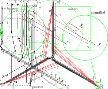
(b)

(c)

(d)

Figure 15: Constructing $\Gamma$ from $\Pi$ for the proof of Theorem 2.

We now describe the procedure to construct $\Gamma$ from $\Pi$ in detail. We will make sure that all vertices of $\Gamma$ have rational coordinates with numerators and denominators in $O(n^{2})$. Let $V_{1}=\{u_{1},\dots,u_{q}\}$, $V_{2}=\{v_{1},\dots,v_{q}\}$ and $V_{3}=\{w_{1},\dots,w_{q}\}$. For the construction, we introduce dummy points $u_{0}^{\Gamma}$, $u_{q+1}^{\Gamma}$, $v_{0}^{\Gamma}$, $v_{q+1}^{\Gamma}$, $w_{0}^{\Gamma}$, $w_{q+1}^{\Gamma}$, which do not lie on $\Gamma$. For all $i=0,\dots,q+1$, it will be $|ou_{i}^{\Gamma}|=|ov_{i}^{\Gamma}|=|ow_{i}^{\Gamma}|$.

We first show how to choose coordinates for points $o,u_{0}^{\Gamma},\dots,u_{q+1}^{\Gamma}$; see Fig. 15a. We approximate $120^{\circ}$ rotation using the angle $\alpha\approx 120.51^{\circ}$ with $\cos\alpha=-\frac{33}{65}$ and $\sin\alpha=\frac{56}{65}$. The points $v_{i}^{\Gamma}$ are acquired from $u_{i}^{\Gamma}$ by a clockwise rotation by $\alpha$ at $o$, and the points $w_{i}^{\Gamma}$ are acquired from $u_{i}^{\Gamma}$ by a counterclockwise rotation by $\alpha$ at $o$. Then, $\angle u_{i}^{\Gamma}ov_{i}^{\Gamma}=\angle u_{i}^{\Gamma}ow_{i}^{\Gamma}=\alpha$ and $\angle v_{i}^{\Gamma}ow_{i}^{\Gamma}=360^{\circ}-2\alpha\approx 118.98^{\circ}$.

Let point $o$ have coordinates $(0,0)$. For $i=1,\dots,q$, let the first segment of the $o$-$u_{i}^{\Gamma}$ path have its other endpoint in $(i,c_{1}q)$ for a constant $c_{1}$. For $i=0,\dots,i+1$, point $u_{i}^{\Gamma}$ has $x$-coordinate $i$. Let $y_{i}$ denote the $y$-coordinate of $u_{i}^{\Gamma}$. We set $y_{0}=c_{1}q+c_{2}q^{2}$ for a constant $c_{2}$. For $i=1,\dots,q$, we set $y_{i}=y_{i-1}+2q+1-i$; see Fig. 15a. Thus, for $i=0,\dots,q+1$, points $u_{i}^{\Gamma}$ lie on a parabola that opens down. Note that all vertices of $\Gamma$ constructed so far are integers in $O(n^{2})$. We set $c_{1}=5$ and $c_{2}=40$.

Next, we show how to construct the dents on the $o$-$u_{i}^{\Gamma}$ paths. For edge $u_{i}v_{j}$ in $G$, $i,j=1,\dots,q$, consider the straight line through $v_{j-1}^{\Gamma}v_{j+1}^{\Gamma}$; see the dashed red line in Fig. 15b for $j=3$. Consider the intersection of this line and the vertical line through $u_{i}^{\Gamma}$. The coordinates of that intersection are rational numbers with numerators and denominators in $O(n^{2})$. It is easy to show that this intersection has $y$-coordinates between $\frac{c_{2}}{2}q=20q$ and $\frac{6}{5}(c_{1}+c_{2}q+\frac{3}{2}(q+1))<8+50q$.

At the intersection, we place a dent consisting of two segments; see Fig. 15c. The first segment of the dent has positive slope and is orthogonal to $v_{j-1}^{\Gamma}v_{j+1}^{\Gamma}$. Its projection on the $x$ axis has length $\frac{1}{2}$. The second segment has the negative slope of $-5$. It is easy to verify that the line through $v_{j}^{\Gamma}v_{j+2}^{\Gamma}$ (the upper red dashed line in Fig. 15c) has distance at least $\frac{c_{2}}{8}=5$ from the lowest point of the dent. Therefore, the dent fits between the two dashed red lines. Note that all three vertices of the dent have coordinates that are rational numbers with numerators and denominators in $O(n^{2})$.

By the choice of the slopes, no normal to either one of the dent segments crosses $ow_{k}^{\Gamma}$ for $k=0,\dots,q+1$. Furthermore, no normal on the second segment crosses $ov_{k}^{\Gamma}$ for $k=0,\dots,q+1$, and a normal to the first segment only crosses $ov_{k}^{\Gamma}$ for $k=j$. In this way, the dent ensures that $u_{i}^{\Gamma}$ and $v_{j}^{\Gamma}$ can not be in the same GRR, and it does not prohibit any other vertex pair ($u_{k}^{\Gamma}$ and $v_{\ell}^{\Gamma}$, $v_{k}^{\Gamma}$ and $w_{\ell}^{\Gamma}$, $w_{k}^{\Gamma}$ and $v_{\ell}^{\Gamma}$, $k,\ell=1,\dots,q$) from being in the same GRR. Finally, for each leaf vertex $u_{i}^{\Gamma}$, we add the missing segments on the vertical line through $u_{i}^{\Gamma}$ to connect $o$ and $u_{i}^{\Gamma}$ by a path. Analogously, we construct the $o$-$v_{i}^{\Gamma}$ and the $o$-$w_{i}^{\Gamma}$ paths.

Note that by our construction, the dent normals do not cross other dents on the paths from $o$ to the leaves from another partition; see Fig. 15d, where the dents lie in the dark gray rectangles, and the crossings of dent normals and paths from $o$ to the leaves from another partition lie in the light gray rectangles. It follows that for $i,j=1,\dots,q$, the $o$-$u_{i}^{\Gamma}$ and the $o$-$v_{j}^{\Gamma}$ path can be merged into one GRR, if no dent corresponding to edge $u_{i}v_{j}$ in $G$ exists on the $o$-$u_{i}^{\Gamma}$ path in $\Gamma$.

From the construction of $\Gamma$, it follows that a pair of leaves $x^{\Gamma}$ and $y^{\Gamma}$ can be in the same GRR if and only if the corresponding vertices $x,y$ are in different partitions of $V$ and edge $xy$ is not in $G$. Therefore, triples of leaves $x^{\Gamma},y^{\Gamma},z^{\Gamma}$ for which $x^{\Gamma},y^{\Gamma},z^{\Gamma}$ can be in the same GRR, are in one to one correspondence to independent triples from $V_{1}\times V_{2}\times V_{3}$ in $G$. Therefore, $\Gamma$ can be partitioned into $q$ GRRs if and only if $\Pi$ is a yes-instance of PIIT. Note that $\Gamma$ can be constructed in polynomial time and that all coordinates of vertices in $\Gamma$ are rational numbers with numerators and denominators in $O(n^{2})$. ∎

4.2 Polynomial-time algorithms for restricted types of contacts

We now make a restriction by only allowing non-crossing contacts.

First, assume $T$ is split only at its vertices. As shown in Section 2.2, we can drop this restriction and adapt our algorithms to compute minimum or approximately minimum GRR decompositions of plane straight-line tree drawings which allow splitting tree edges at interior points. Note that the construction in the proof of Lemma 3 preserves the non-crossing property of GRR contacts.

We start in Section 4.2.1 and use the well-known problem Minimum Multicut to compute a 2-approximation for minimum GTDs for the scenario in which GRRs are only allowed to have proper contacts. A similar approach will be used in Section 5 to compute minimum GRR decompositions of triangulated polygons. After that, in Section 4.2.2, we present an exact, but more complex approach for computing GTDs, which also allows non-crossing contacts.

4.2.1 2-Approximation using Multicut

(a)

(b)

Figure 16: LABEL:sub@fig:trees:minmult-1 Tree drawing decomposed in GRRs. Edge pairs $\{e_{1},e_{2}\}$, …, $\{e_{4},e_{5}\}$, $\{e_{5},e_{1}\}$ as well as $\{e_{1},e_{6}\}$, $\{e_{4},e_{6}\}$ are conflicting. LABEL:sub@fig:trees:minmult-2 Minimum Multicut instance constructed according to the proof of Proposition 5. No edge orientation respecting all paths between the terminals exists. Dashed edges form a solution.

We show how to partition the edges of $T$ into a minimum number of increasing-chord components with proper contacts using Minimum Multicut on trees. Given an edge-weighted graph $G=(V,E)$ and a set of terminal pairs $\{(s_{1},t_{1})$, …,$(s_{k},t_{k})\}$, an edge set $S\subseteq E$ is a multicut if removing $S$ from $G$ disconnects each pair $s_{i},t_{i}$, $i=1,\dots,k$. A multicut is minimum if the total weight of its edges is minimum.

For the complexity of Minimum Multicut on special graph types, see the survey by Costa et al. [7]. Computing Minimum Multicut is $\NP$-hard even for unweighted binary trees [3], but has a polynomial-time 2-approximation for trees [11].

Consider a plane straight-line drawing of a tree $T=(V,E)$. We construct a tree $T_{M}$ by subdividing every edge of $T$ once as follows. Tree $T_{M}$ has a vertex $n_{v}$ for each vertex $v\in V$ and a vertex $n_{e}$ for each edge $e\in E$. For each $e=uv\in E$, edges $n_{u}n_{e}$ and $n_{e}n_{v}$ are in $T_{M}$. The set $X$ of terminal pairs contains a pair $(n_{e},n_{f})$ for each pair of conflicting edges $e,f$ of $T$. Let all edges of $T_{M}$ have weight 1.

Lemma 5.

Let $E^{\prime}$ be a Minimum Multicut of $T_{M}$ with respect to the terminal pairs $X$ and let $C_{1}^{M},\dots,C_{k}^{M}$ denote the connected components of $T_{M}-E^{\prime}$. Then, components $C_{i}=\{e\in E\mid n_{e}\in C_{i}^{M}\}$ form a minimum GRR decomposition of $T$.

Proof.

Consider a multicut $E^{\prime}$ of $T_{M}$, $|E^{\prime}|=k-1$. Consider a component $C_{i}^{M}$. Then, the edges in $C_{i}$ are conflict-free and form a connected subtree $T_{i}$ of $T$. Thus, $T_{i}$ is a GRR by Lemma 2.

Next, consider a GRR decomposition of $T$ into $k$ subtrees $T_{i}=(V_{i},E_{i})$ with proper contacts. We create an edge set $S$ as follows. Assume $T_{i}$, $T_{j}$ touch at vertex $v\in V$. Let edge $e=uv$ be in $T_{i}$, and let $v$ be a leaf in $T_{i}$. Then we add edge $n_{e}n_{v}$ of $T_{M}$ to set $S$; see Fig. 16a and 16b. It is $|S|=k-1$. After removing $S$ from $T_{M}$, no connected component contains vertices $n_{e_{1}},n_{e_{2}}$ for a pair of conflicting edges $e_{1}$, $e_{2}$. Thus, $S$ is a multicut.

We have shown that GRR decompositions of $T$ of size $k$ are in one-to-one correspondence with the multicuts of $T_{M}$ of size $k-1$. Therefore, minimum multicuts correspond to minimum GRR decompositions, and it follows that $C_{i}$ form a minimum GRR decomposition of $T$. ∎

Note that Minimum Multicut can be solved in polynomial time in directed trees [6], i.e., trees whose edges can be directed such that for each terminal pair $(s_{i},t_{i})$, the $s_{i}$-$t_{i}$ path is directed. We note that this result cannot be applied in our context, since we can get Minimum Multicut instances for which no such orientation is possible, see Fig. 16b. However, using the approximation algorithm from [11], we obtain the following result.

Corollary 1.

Given a plane straight-line drawing of a tree $T=(V,E)$, a partition of $E$ into $2\cdot\textnormal{OPT}-1$ increasing-chord subtrees of $T$ having only proper contacts can be computed in time polynomial in $n$, where OPT is the minimum size of such a partition.

4.2.2 Optimal solution

In the following we show how to find a minimum GRR partition with only non-crossing contacts in polynomial time. As is the case with minimum partitions of simple hole-free polygons into convex [4] or star-shaped [13] components, our algorithm is based on dynamic programming. We describe the dynamic program in detail and use it to find minimum GTDs for the setting as in Section 4.2.1, as well as for the setting in which non-proper, but non-crossing contacts of GRRs are allowed. First, we shall prove the following theorem.

Theorem 3.

Given a plane straight-line drawing of a tree $T=(V,E)$, a partition of $E$ into a minimum number of increasing-chord subtrees of $T$ (minimum GTD) having only non-crossing contacts can be computed in time $O(n^{6})$.

At the end of Section 4.2.2, we modify our dynamic program slightly to prove Theorem 4, which shows the same result for the setting in which only partitions with proper contacts are considered.

Theorem 4.

Given a plane straight-line drawing of a tree $T=(V,E)$, a partition of $E$ into a minimum number of increasing-chord subtrees of $T$ (minimum GTD) having only proper contacts can be computed in time $O(n^{6})$.

Let $T$ be rooted. For each vertex $u$ with parent $\pi_{u}$, let $T_{u}$ be the subtree of $u$ together with edge $\pi_{u}u$. We shall use the following definition.

Definition 10 (root component).

Given a GRR partition of the edges of a rooted tree $T^{\prime}$, we call all GRRs containing the root of $T^{\prime}$ the root components. If the root of $T^{\prime}$ has degree 1, every GRR partition of $T^{\prime}$ has one unique root component.

A minimum partition is constructed from the solutions of subinstances as follows. Let $u_{1},\dots,u_{d}$ be the children of $u$. For subtrees $T_{u_{1}}$, …, $T_{u_{d}}$ whose only common vertex is $u$, a minimum partition $P^{\prime}$ of $T^{\prime}=\bigcup_{i}T_{u_{i}}$ induces partitions $P_{i}$ of $T_{u_{i}}$. Furthermore, $P^{\prime}$ is created by choosing $P_{i}$ as partitions of $T_{u_{i}}$ and possibly merging some of the root components of $T_{u_{i}}$, $i=1,\dots,d$. Note that $P_{i}$ is not necessarily a minimum partition of $T_{u_{i}}$, if $P_{i}$ allows us to merge more root components than a minimum partition of $T_{u_{i}}$ would allow. Therefore, for every $u$ we shall store minimum partitions of $T_{u}$ for various possibilities of the root component of $T_{u}$. For the sake of uniformity, we choose a vertex with degree 1 as the root of $T$.

Given a tree root, the number of different subtrees it could be contained in may be exponential, e.g., it is $\Theta(2^{n})$ in a star. The key observation for our algorithm is that we do not need to store a partition for each possible root component. We require the following notation.

Definition 11 (Path clockwise between).

Consider directed non-crossing paths $\rho_{1}$, $\rho_{2}$, $\rho_{3}$ with common origin $r$, endpoints $t_{1}$, $t_{2}$, $t_{3}$ and, possibly, common prefixes. Let $V_{i}$ be vertices of $\rho_{i}$, $i=1,2,3$, and let $T$ be the tree formed by the union of $\rho_{1},\rho_{2}$ and $\rho_{3}$. We say that $\rho_{2}$ is clockwise between $\rho_{1}$ and $\rho_{3}$, if the clockwise traversal of the outer face of $T$ visits $t_{1}$, $t_{2}$, $t_{3}$ in this order; see Fig. 17a.

Note that in Definition 11 the three paths may (partially) coincide. Lemma 6 shows that to decide whether a union of two subtrees is increasing-chord, it is sufficient to consider only the two pairs of “outermost” root-leaf paths of each subtree. This result is crucial for limiting the number of representative decompositions that need to be considered during our dynamic programming approach. The statement of the lemma is illustrated in Fig. 17b.

(a)

(b)

Figure 17: LABEL:sub@fig:path-clockwise-between Path $\rho_{2}$ is clockwise between paths $\rho_{1}$ and $\rho_{3}$. LABEL:sub@fig:trees:combine:paths Statement of Lemma 6.

Lemma 6.

Let $T_{1}$, $T_{2}$ be increasing-chord trees sharing a single vertex $r$. Let all tree edges be directed away from $r$. Let paths $\rho_{1}$, $\rho_{2}$ in $T_{1}$ and $\rho_{3}$, $\rho_{4}$ in $T_{2}$ be paths from $r$ to a leaf, such that:

1. every directed path from $r$ in $T_{1}$ is clockwise between $\rho_{1}$ and $\rho_{2}$;

2. every directed path from $r$ in $T_{2}$ is clockwise between $\rho_{3}$ and $\rho_{4}$;

3. for $i=1,\dots,4$, path $\rho_{i}$ is clockwise between $\rho_{i-1}$ and $\rho_{i+1}$ (indices modulo 4).

Then, $\rho_{1}\cup\rho_{2}\cup\rho_{3}\cup\rho_{4}$ is increasing-chord if and only if $T_{1}\cup T_{2}$ is increasing-chord.

Proof.

Consider trees $T_{1}$, $T_{2}$ and paths $\rho_{1},\dots,\rho_{4}$ satisfying the condition of the lemma; see Fig. 17b for a sketch. Note that $\rho_{1}$ and $\rho_{2}$ may have common prefixes, and so may $\rho_{3}$ and $\rho_{4}$. Assume the four paths $\rho_{1},\dots,\rho_{4}$ are drawn with increasing chords, but the union $T^{\prime}$ of the trees $T_{1}$ and $T_{2}$ is not. Then, there exist edges $u_{1}v_{1}$ in $T_{1}$ and $u_{4}v_{4}$ in $T_{2}$, such that the normal $\ell$ to $u_{1}v_{1}$ at $u_{1}$ crosses edge $u_{4}v_{4}$.

(a)

(b)

Figure 18: Constructions in Lemma 6.

Claim 1.

Without loss of generality, we may assume the following; see Fig. 18. (i) Edge $u_{1}v_{1}$ points vertically upwards, (ii) edge $u_{4}v_{4}$ is the first edge on the $r$-$v_{4}$ path $\rho^{\prime\prime}$ crossed by $\ell$ and points upwards, (iii) vertex $u_{4}$ is on $\ell$ and to the right of $u_{1}$.

We ensure (i) by rotation. Then, point $r$ is below $\ell$ (or on it), since the $r$-$v_{1}$ path $\rho^{\prime}$ is increasing-chord. For (ii), we choose $u_{4}v_{4}$ as the first edge with this property. If it points downward, there is an edge on the $r$-$u_{4}$ path crossed by $\ell$. For (iii), if $\ell$ crosses $u_{4}v_{4}$ in an interior point $p$, we subdivide the edge at $p$ and replace $u_{4}v_{4}$ by $pv_{4}$. If $u_{4}$ is left of $u_{1}$, we mirror the drawing horizontally. This proves the claim.

First, assume that $v_{1}$, $v_{4}$ are not on paths $\rho_{1},\dots,\rho_{4}$. Recall that two of the paths $\rho_{1},\dots,\rho_{4}$ (without loss of generality, $\rho_{2}$ and $\rho_{3}$) are between $\rho^{\prime}$ and $\rho^{\prime\prime}$. Let $u_{2}v_{2}$ and $u_{3}v_{3}$ be the last two edges on $\rho_{2}$ and $\rho_{3}$, respectively. Note that $\textnormal{ray}(u_{1},v_{1})$ and $\textnormal{ray}(u_{2},v_{2})$ must diverge, and so must $\textnormal{ray}(u_{2},v_{2})$ and $\textnormal{ray}(u_{3},v_{3})$. If $u_{4}v_{4}$ points upwards and to the left as in Fig. 18a, then $\textnormal{ray}(u_{3},v_{3})$ and $\textnormal{ray}(u_{4},v_{4})$ must converge; a contradiction. Thus, $u_{2}v_{2}$, $u_{3}v_{3}$ and $u_{4}v_{4}$ point upwards and to the right; see Fig. 18b. Since $T_{1}$ as well as the union of $\rho_{1}$ and $\rho_{2}$ is increasing-chord, the angles $\angle v_{1}u_{1}u_{2}$, $\angle u_{1}u_{2}v_{2}$, $\angle v_{2}u_{2}u_{3}$ and $\angle u_{2}u_{3}v_{3}$ are between $90^{\circ}$ and $180^{\circ}$. Therefore, vertices $u_{2}$ and $u_{3}$ must lie below $\ell$. Let $\ell_{3}$ be the normal to $u_{3}v_{3}$ at $u_{3}$. Since $T_{2}$ is drawn with increasing chords, $u_{4}v_{4}$ must lie below $\ell_{3}$, a contradiction.

The proof works similarly if $u_{1}v_{1}$ is on $\rho_{2}$ (by identifying $u_{1}v_{1}$ and $u_{2}v_{2}$), and the remaining cases are symmetric. ∎

We now describe our dynamic programs for proper and non-crossing contacts in detail. We first give an overview of the general approach, then describe the non-crossing case and afterwards modify it for proper contacts. For a root component $R$ of $T_{u}$, let the leftmost path (or, respectively, the rightmost path) be the simple path in $R$ starting at $\pi_{u}$ which always chooses the next counterclockwise (clockwise) edge.

The basic idea of the dynamic program is as follows. For a given subtree $T_{u}$, we store the sizes of the minimum GTDs of $T_{u}$ for different possibilities of the root component. We combine these solutions to compute minimum GTDs of bigger subtrees. For this step, we must be able to test which root components can be merged into one GRR. Instead of storing the partition sizes for all possible root components, we only store the minimum partition size for each combination of the leftmost and rightmost path of the root component. Thus, for each $T_{u}$, we only store $O(n^{2})$ partition sizes. Note that this is sufficient, since by Lemma 6 the question whether two root components can be merged depends only on their leftmost and rightmost paths.

If $u$ is the root of a subtree $T^{\prime}$ and has degree 2 or greater in $T^{\prime}$, there might be several root components in a partition of $T^{\prime}$, i.e., GRRs containing $u$. Let $R$ be some fixed root component of the considered GTD. If $u$ has degree 2 or greater in $R$, then we need a reference direction to define the leftmost and rightmost paths of $R$. Let $\rho_{l}$ be the leftmost path of the rooted tree $R+\pi_{u}u$. Note that $\rho_{l}$ contains the edge $\pi_{u}u$. Then, the leftmost path of $R$ is $\rho_{l}-\pi_{u}u$. The rightmost path of $R$ is defined analogously.

Recall that $T_{u}$ is the subtree of $u$ together with edge $\pi_{u}u$. For each pair of vertices $t_{i},t_{j}$ in $T_{u}$, cell $\tau[u,t_{i},t_{j}]$ of a table $\tau$ stores the size of a minimum GRR decomposition of $T_{u}$, in which the root component has the $\pi_{u}$-$t_{i}$ path and the $\pi_{u}$-$t_{j}$ path as its leftmost and rightmost path, respectively. Cell $\tau[u]$ stores the size of a minimum GRR decomposition of $T_{u}$. It is $\tau[u]=\min_{t_{i},t_{j}}\tau[u,t_{i},t_{j}]$. For simplicity, we set $\min\emptyset=\infty$.

Clearly, for each leaf $u$, $\tau[u,u,u]=1$, and $\tau[u,t_{i},t_{j}]=\infty$ for all other values of $t_{i},t_{j}$. Let $v$ be the only neighbor of the root $r$ of the tree $T$. Then, $\tau[v]$ is the size of a minimum GRR decomposition of $T$. We show how to compute $\tau$ bottom-up.

For ease of presentation, we use the following notation. Vertex $u$ is not a leaf and has children $u_{1},\dots,u_{d}$. Let $\pi_{u}$, $u_{1}$, …, $u_{d}$ have this clockwise order around $u$. Let $t_{i}\neq u$ be a vertex in $T_{u_{i}}$. We define $t_{j},t_{k},t_{\ell}$ analogously for $1\leq i\leq j\leq k\leq\ell\leq d$. Let $\rho_{i}$ be the $u$-$t_{i}$ path.

We consider two settings: allowing arbitrary non-crossing contacts and allowing only proper contacts. The dynamic programs for the two cases are very similar, and the program for arbitrary non-crossing contacts is slightly more complex. To reduce duplication, we first present the program for arbitrary non-crossing contacts, and later show how to modify it for the case when only proper contacts are allowed.

4.2.3 Non-crossing contacts

Recall that vertex $u$ can live in a root component $R$ together with non-consecutive children $u_{i}$, $u_{\ell}$, $i<\ell$. If arbitrary non-crossing contacts are allowed, some nodes from $u_{i+1},\dots,u_{\ell-1}$ that are not in $R$ can also be in one GRR. Therefore, after choosing the root component $R$ of $T_{u}$, we must be able to recursively compute the minimum size of a partition of the union of $T_{u_{j}}$, $u_{j}\notin R$. We introduce additional tables for this purpose.

In addition to the table $\tau$ storing the values $\tau[u,t_{i},t_{j}]$, we use tables $\sigma_{\Delta}$ for $\Delta=1,\dots,4$, as well as tables $\sigma$ and $\sigma_{M}$. These additional tables will be used to formulate the recurrences for $\tau$. For fixed $u$, $i$, $j$, the corresponding values of $\sigma_{\Delta}$, $\sigma$ and $\sigma_{M}$ denote the sizes of minimum GTDs of $T_{u_{i}}\cup T_{u_{i+1}}\cup\dots\cup T_{u_{j}}$ with certain properties. Table $\sigma_{\Delta}$ considers different possibilities of the leftmost and rightmost paths of the root components as well as the degree $\Delta$ of $u$ in the root component. Recall that in an increasing-chord tree drawing, every vertex has degree at most 4. Formally, the value $\sigma_{\Delta}[u,t_{i},t_{j}]$ denotes the minimum number of GRRs in a GTD of the tree $T_{u_{i}}\cup T_{u_{i+1}}\cup\dots\cup T_{u_{j}}$, in which there exists a GRR $R$ with the rightmost path $u$-$t_{i}$ and leftmost path $u$-$t_{j}$ and in which $u$ has degree $\Delta$ in $R$.

For some recurrences, we need to aggregate the various possibilities stored in $\sigma_{\Delta}$. For this purpose, we use tables $\sigma$ and $\sigma_{M}$ as follows. The value $\sigma$ is the minimum of $\sigma_{\Delta}$ over all values of $\Delta$. We define $\sigma[u,t_{i},t_{j}]$ as $\sigma[u,t_{i},t_{j}]=\min_{\Delta=1,\dots,4}\sigma_{\Delta}[u,t_{i},t_{j}]$.

The value $\sigma_{M}$ stores the minimum over all combinations of the leftmost and rightmost paths. Thus, it stores the size of the minimum partition of $T_{u_{i}}\cup\dots\cup T_{u_{j}}$, regardless of the root component. Formally, $\sigma_{M}[u,i,j]$ denotes the minimum number of GRRs in a GTD of $T_{u_{i}}\cup\dots\cup T_{u_{j}}$. Note that the arguments of $\sigma_{M}[u,\cdot,\cdot]$ are indices $i$, $j$ of a pair of children of $u$, and the arguments of $\sigma_{\Delta}[u,\cdot,\cdot]$ and $\sigma[u,\cdot,\cdot]$ are a pair of vertices in $T_{u_{i}}\cup\dots\cup T_{u_{j}}$.

In the following recurrences, for a fixed pair of vertices $t_{i}$ and $t_{\ell}$, all possibilities for $t_{j}$ and $t_{k}$ are considered, such that both paths $\rho_{j}$ and $\rho_{k}$ are clockwise between $\rho_{i}$ and $\rho_{\ell}$. We test whether root components $R_{1}$ with the leftmost and rightmost paths $\rho_{i}$ and $\rho_{j}$ and $R_{2}$ with the leftmost and rightmost paths $\rho_{k}$ and $\rho_{\ell}$ can be merged to a single GRR. We show that this covers all representative possibilities for a root component of a GTD of $T_{u_{i}}\cup\dots\cup T_{u_{\ell}}$ to have the leftmost and rightmost paths $\rho_{i}$ and $\rho_{\ell}$, respectively.

Lemma 7.

We have the recurrences

1. $\sigma_{1}[u,t_{i},t_{j}]=\sigma[u,t_{i},t_{j}]=\tau[u_{i},t_{i},t_{j}]$ for all $t_{i},t_{j}\neq u$ in $T_{u_{i}}$, $i=1,\dots,d$;

2. $\sigma_{M}[u,i,i]=\tau[u_{i}]$ for all $i=1,\dots,d$;

3. $\sigma_{2}[u,t_{i},t_{\ell}]=\min_{t_{j},t_{k}}\{\sigma_{1}[u,t_{i},t_{j}]+\sigma_{M}[u,j+1,k-1]+\sigma_{1}[u,t_{k},t_{\ell}]-1\}$;

4. $\sigma_{3}[u,t_{i},t_{\ell}]=\min\{\min_{t_{j},t_{k}}\{\sigma_{2}[u,t_{i},t_{j}]+\sigma_{M}[u,j+1,k-1]+\sigma_{1}[u,t_{k},t_{\ell}]-1\},$

   $\min_{t_{j},t_{k}}\{\sigma_{1}[u,t_{i},t_{j}]+\sigma_{M}[u,j+1,k-1]+\sigma_{2}[u,t_{k},t_{\ell}]-1\}\}$;

5. $\sigma_{4}[u,t_{i},t_{\ell}]=\min_{t_{j},t_{k}}\{\sigma_{1}[u,t_{i},t_{i}]+\sigma_{M}[u,i+1,j-1]+\sigma_{1}[u,t_{j},t_{j}]$

   $+\sigma_{M}[u,j+1,k-1]+\sigma_{1}[u,t_{k},t_{k}]+\sigma_{M}[u,k+1,\ell-1]+\sigma_{1}[u,t_{\ell},t_{\ell}]\}-3$.

The minimizations in lines ((7)) and ((9)) only consider vertices $t_{j},t_{k}$, such that $\rho_{i}\cup\rho_{j}\cup\rho_{k}\cup\rho_{\ell}$ is increasing-chord.

(a)

(b)

(c)

Figure 19: Recurrences in Lemma 7. LABEL:sub@fig:noncrossing:rec:1 recurrence ((1)); LABEL:sub@fig:noncrossing:rec:2 recurrence ((5)) for the case $m=j$; LABEL:sub@fig:noncrossing:rec:2 recurrence ((5)) for the case $m=k$.

Proof.

Consider recurrence ((1)) and a GTD of $T_{u_{i}}\cup\dots\cup T_{u_{j}}$ of size $x$ with root component $R$, such that $R$ has $u$-$t_{i}$ and $u$-$t_{j}$ as its leftmost and rightmost paths, respectively. Since $u$ has degree $1$ in $R$, it must be $i=j$. Thus, this partition is a GTD of $T_{u_{i}}$ with $R$ as the root component, so by definition of $\tau$ we have $\tau[u,t_{i},t_{j}]\leq x$. Thus, we have $\sigma_{1}[u,t_{i},t_{j}]\geq\tau[u_{i},t_{i},t_{j}]$. Conversely, consider a GTD of $T_{u_{i}}$, such that its root component $R$ has $u$-$t_{i}$ and $u$-$t_{j}$ as its leftmost and rightmost paths. Thus, $t_{i}$ and $t_{j}$ are both in $T_{u_{i}}$, and vertex $u$ has degree $1$ in $R$. By the definition of $\sigma_{1}$, this partition has size at least $\sigma_{1}[u,t_{i},t_{j}]$. Thus, we have $\sigma_{1}[u,t_{i},t_{j}]\leq\tau[u_{i},t_{i},t_{j}]$. Finally, since for $i=j$ we have $T_{u_{i}}\cup\dots\cup T_{u_{j}}=T_{u_{i}}$, vertex $u$ can only have degree $1$ in the root component of a GTD, so we have $\sigma_{1}[u,t_{i},t_{j}]=\sigma[u,t_{i},t_{j}]$. Thus, recurrence ((1)) holds.

Recurrence ((3)) holds trivially, since by the definitions of $\sigma_{M}$ and $\tau[\cdot]$, both $\sigma_{M}[u,i,i]$ and $\tau[u_{i}]$ denote the size of the minimum GRR partition of $T_{u_{i}}$.

Consider recurrence ((5)) and a GTD $P$ of $T_{u_{i}}\cup\dots\cup T_{u_{\ell}}$ of size $x$ with root component $R$. Again, let $R$ have $u$-$t_{i}$ and $u$-$t_{\ell}$ as its leftmost and rightmost paths, respectively. Let $u$ have degree $2$ in $R$. Therefore, $i\neq\ell$, and $R$ only consists of two parts $R_{1},R_{2}$ (green and blue in Fig. 19a, respectively), such that $R_{1}$ is contained in $T_{u_{i}}$ and $R_{2}$ is contained in $T_{u_{\ell}}$. Partition $P$ induces a GTD $P_{1}$ of $T_{u_{i}}$ of size $x_{1}$, a GTD $P_{2}$ of $T_{u_{\ell}}$ of size $x_{2}$ and a GTD $P_{3}$ of $T_{u_{i+1}}\cup\dots\cup T_{u_{\ell-1}}$ of size $x_{3}$. Since $R_{1}\cup R_{2}=R$, we have $x=x_{1}+x_{2}+x_{3}-1$. Let $u_{j}$ be a vertex in $R_{1}$, such that $u$-$u_{j}$ is the rightmost path of $R_{1}$. Let $u_{k}$ be the vertex in $R_{2}$, such that $u$-$u_{k}$ is the leftmost path of $R_{2}$. The subtree $\rho_{i}\cup\rho_{j}\cup\rho_{k}\cup\rho_{\ell}$ is contained in $R$ and, therefore, is increasing-chord. By the definition of $\sigma_{1}$ and $\sigma_{M}$, we have $\sigma_{1}[u,t_{i},t_{j}]\leq x_{1}$, $\sigma_{1}[u,t_{k},t_{\ell}]\leq x_{2}$ and $\sigma_{M}[u,j+1,k-1]\leq x_{3}$. Thus, the right part of recurrence ((5)) is at most $x$, so the right side is upper bounded by the left side.

Conversely, let the right side of recurrence ((5)) be less than $\infty$. Let $j,k$, $t_{j},t_{k}$ be chosen such that the minimum on the right side is realized. Then, $\rho_{i}\cup\rho_{j}\cup\rho_{k}\cup\rho_{\ell}$ is increasing-chord. Let $\sigma_{1}[u,t_{i},t_{j}]=x_{1}$, and let $P_{1}$ be a GTD of size $x_{1}$ realizing the minimum in the definition of $\sigma_{1}[u,t_{i},t_{j}]$. Let $R_{1}$ be the root component of $P_{1}$. Then, $R_{1}$ has leftmost and rightmost paths $u$-$t_{i}$ and $u$-$t_{j}$ respectively. Analogously, let $\sigma_{1}[u,t_{k},t_{\ell}]=x_{2}$, and let $P_{2}$ be a GTD of size $x_{2}$ realizing the minimum in the definition of $\sigma_{1}[u,t_{k},t_{\ell}]$. Let $R_{2}$ be the root component of $P_{2}$. Then, $R_{2}$ has leftmost and rightmost paths $u$-$t_{k}$ and $u$-$t_{\ell}$ respectively. Finally, let $P_{3}$ be a GTD of size $x_{3}$ realizing the minimum in the definition of $\sigma_{M}[u,j+1,k-1]$. By Lemma 6, $R_{1}\cup R_{2}$ is increasing-chord. Consider the GTD $P$ formed by taking the union of $P_{1}$, $P_{2}$ and $P_{3}$ and merging $R_{1}$ and $R_{2}$. Partition $P$ has size $x_{1}+x_{2}+x_{3}-1$. Its root component $R$ has leftmost and rightmost paths $u$-$t_{i}$ and $u$-$t_{\ell}$ respectively, and $u$ has degree 2 in $R$. Thus, by the definition of $\sigma_{2}[u,t_{i},t_{\ell}]$, it is $\sigma_{2}[u,t_{i},t_{\ell}]\leq x_{1}+x_{2}+x_{3}-1$. Thus, the left side of recurrence ((5)) is upper bounded by its right side. Therefore, recurrence ((5)) holds.

Next, consider recurrence ((7)) and a GRR partition $P$ of $T_{u_{i}}\cup\dots\cup T_{u_{\ell}}$ of size $x$ with root component $R$. Once again, let $R$ have $u$-$t_{i}$ and $u$-$t_{\ell}$ as its leftmost and rightmost paths, respectively. Let $u$ have degree $3$ in $R$. Therefore, it is $i\neq\ell$. In addition to $u_{i}$ and $u_{\ell}$, the GRR $R$ must contain another child $u_{m}$ of $u$, such that $i<m<\ell$. We can partition $R$ into two GRRs $R_{1}$ and $R_{2}$, such that $u_{i}$ is in $R_{1}$, $u_{\ell}$ in $R_{2}$ and $u_{m}$ is either in $R_{1}$ or in $R_{2}$. First, assume $u_{m}$ is in $R_{1}$; see Fig. 19b. The other case is symmetric; see Fig. 19c. We choose $j=m$. Let $t_{j}$ be a vertex in $T_{u_{j}}$, such that $u$-$t_{j}$ is the rightmost path of $R_{1}$. Let $t_{k}$ be a vertex in $T_{u_{\ell}}$, such that $u$-$t_{k}$ is the leftmost path in $R_{2}$. Note that in this case, $t_{k}$ and $t_{\ell}$ are in the same subtree $T_{u_{k}}=T_{u_{\ell}}$. We can split the partition $P$ into GRR partitions $P_{1}$ of $T_{u_{i}}\cup\dots\cup T_{u_{j}}$ of size $x_{1}$, $P_{2}$ of $T_{u_{\ell}}$ of size $x_{2}$ and $P_{3}$ of $T_{u_{j+1}}\cup\dots\cup T_{u_{k-1}}$ of size $x_{3}$. It holds: $R=R_{1}\cup R_{2}$, and apart from $R$, no other GRR in $P$ is split, since the contacts are non-crossing. Thus, it is $x=x_{1}+x_{2}+x_{3}-1$. By definition, $\sigma_{2}[u,t_{i},t_{j}]\leq x_{1}$, $\sigma_{1}[u,t_{k},t_{\ell}]\leq x_{2}$ and $\sigma_{M}[u,j+1,k-1]\leq x_{3}$. Therefore, the right side of recurrence ((7)) is at most $x$. The same holds for the symmetric case in which $u_{m}$ is in $R_{2}$ by analogous arguments. Thus, the right side of recurrence ((7)) is upper bounded by its left side.

Conversely, let the right side of recurrence ((7)) be less than $\infty$. Let $j,k$, $t_{j},t_{k}$ be chosen such that the minimum on the right side is realized. First, assume it is realized by $\sigma_{2}[u,t_{i},t_{j}]+\sigma_{M}[u,j+1,k-1]+\sigma_{1}[u,t_{k},t_{\ell}]-1$. Then, $\rho_{i}\cup\rho_{j}\cup\rho_{k}\cup\rho_{\ell}$ is increasing-chord. Let $\sigma_{2}[u,t_{i},t_{j}]=x_{1}$, and let $P_{1}$ be a GRR partition of size $x_{1}$ realizing the minimum in the definition of $\sigma_{2}[u,t_{i},t_{j}]$. Let $R_{1}$ be the root component of $P_{1}$. Then, $R_{1}$ has leftmost and rightmost paths $u$-$t_{i}$ and $u$-$t_{j}$ respectively. The degree of $u$ in $R_{1}$ is $2$, and the vertices $t_{i}$ and $t_{j}$ must lie in different subtrees $T_{u_{i}}$ and $T_{u_{j}}$, respectively. Analogously, let $\sigma_{1}[u,t_{k},t_{\ell}]=x_{2}$, and let $P_{2}$ be a GRR partition of size $x_{2}$ realizing the minimum in the definition of $\sigma_{1}[u,t_{k},t_{\ell}]$. Let $R_{2}$ be the root component of $P_{2}$. Then, $R_{2}$ has leftmost and rightmost paths $u$-$t_{k}$ and $u$-$t_{\ell}$ respectively. Finally, let $P_{3}$ be a GRR partition of size $x_{3}$ realizing the minimum in the definition of $\sigma_{M}[u,j+1,k-1]$. By Lemma 6, $R_{1}\cup R_{2}$ is increasing-chord. Consider the GRR partition $P$ formed by taking the union of $P_{1}$, $P_{2}$ and $P_{3}$ and merging $R_{1}$ and $R_{2}$. Partition $P$ has size $x_{1}+x_{2}+x_{3}-1$. Its root component $R$ has leftmost and rightmost paths $u$-$t_{i}$ and $u$-$t_{\ell}$, respectively, and $u$ has degree 3 in $R$. Therefore, by the definition of $\sigma_{3}[u,t_{i},t_{\ell}]$, it is $\sigma_{3}[u,t_{i},t_{\ell}]\leq x_{1}+x_{2}+x_{3}-1$. Thus, the left side of recurrence ((5)) is upper bounded by its right side. The same holds for the symmetric case in which the minimum on the right side is realized by $\sigma_{1}[u,t_{i},t_{j}]+\sigma_{M}[u,j+1,k-1]+\sigma_{2}[u,t_{k},t_{\ell}]-1$. Therefore, recurrence ((7)) holds.

Finally, consider recurrence ((9)) and a GTD $P$ of $T_{u_{i}}\cup\dots\cup T_{u_{\ell}}$ of size $x$ with root component $R$. Once again, let $R$ have $u$-$t_{i}$ and $u$-$t_{\ell}$ as its leftmost and rightmost paths, respectively. Let $u$ have degree $4$ in $R$. Then, $R$ is a subdivision of $K_{1,4}$ [1]. Let $t_{j}$ and $t_{k}$ be the other two leaves of $R$ lying in the subtrees $T_{u_{j}}$ and $T_{u_{k}}$ respectively, for $1\leq i<j<k<\ell\leq d$. Then, we can split $P$ into $7$ GTDs $P_{1}$, …, $P_{7}$ as follows. Partitions $P_{1}$, $P_{2}$, $P_{3}$, $P_{4}$ are GTDs of subtrees $T_{u_{i}}$, $T_{u_{j}}$, $T_{u_{k}}$ and $T_{u_{\ell}}$, respectively, with the respective sizes $x_{1}$, $x_{2}$, $x_{3}$, $x_{4}$ and paths $u$-$u_{i}$, $u$-$u_{j}$, $u$-$u_{k}$ and $u$-$u_{\ell}$ as the respective root components. Partitions $P_{5}$, $P_{6}$, $P_{7}$ are GTDs of $T_{u_{i+1}}\cup\dots\cup T_{u_{j-1}}$, $T_{u_{j+1}}\cup\dots\cup T_{u_{k-1}}$ and $T_{u_{k+1}}\cup\dots\cup T_{u_{\ell-1}}$, respectively, with respective sizes $x_{5}$, $x_{6}$ and $x_{7}$. The root component $R$ is split into the four paths $u$-$u_{i}$, $u$-$u_{j}$, $u$-$u_{k}$ and $u$-$u_{\ell}$, and no other GRR is split, since the contacts in $P$ are non-crossing. Therefore, it is $x=x_{1}+\dots+x_{7}-3$. By the definition of $\sigma_{1}$, it is $\sigma_{1}[u,t_{i},t_{i}]\leq x_{1}$, $\sigma_{1}[u,t_{j},t_{j}]\leq x_{2}$, $\sigma_{1}[u,t_{k},t_{k}]\leq x_{3}$ and $\sigma_{1}[u,t_{\ell},t_{\ell}]\leq x_{4}$. By the definition of $\sigma_{M}$, $\sigma_{M}[u,i+1,j-1]\leq x_{5}$, $\sigma_{M}[u,j+1,k-1]\leq x_{6}$ and $\sigma_{M}[u,k+1,\ell-1]\leq x_{7}$. Thus, the right side of recurrence ((9)) is at most $x$, so the right side is upper bounded by the left side.

Conversely, let the right side of recurrence ((9)) be less than $\infty$. Let $j,k$, $t_{j},t_{k}$ be chosen such that the minimum on the right side is realized. Then, $\rho_{i}\cup\rho_{j}\cup\rho_{k}\cup\rho_{\ell}$ is increasing-chord. Let $\sigma_{1}[u,t_{i},t_{i}]=x_{1}$, $\sigma_{1}[u,t_{j},t_{j}]=x_{2}$, $\sigma_{1}[u,t_{k},t_{k}]=x_{3}$ and $\sigma_{1}[u,t_{\ell},t_{\ell}]=x_{4}$. Let $P_{1}$, $P_{2}$, $P_{3}$ and $P_{4}$ be GTDs realizing the minimum in the definitions of $\sigma_{1}[u,t_{i},t_{i}]$, $\sigma_{1}[u,t_{j},t_{j}]$, $\sigma_{1}[u,t_{k},t_{k}]$ and $\sigma_{1}[u,t_{\ell},t_{\ell}]$, respectively. Next, let $\sigma_{M}[u,i+1,j-1]=x_{5}$, $\sigma_{M}[u,j+1,k-1]=x_{6}$ and $\sigma_{M}[u,k+1,\ell-1]=x_{7}$. Let $P_{5}$, $P_{6}$ and $P_{7}$ be GTDs realizing the minima in the definitions of $\sigma_{M}[u,i+1,j-1]$, $\sigma_{M}[u,j+1,k-1]$ and $\sigma_{M}[u,k+1,\ell-1]$, respectively. The four paths $\rho_{i}$, $\rho_{j}$, $\rho_{k}$, $\rho_{\ell}$ can be merged into a single GRR $R$ with leftmost path $\rho_{i}$ and rightmost path $\rho_{\ell}$. Consider partition $P$ with root component $R$ formed by taking the union of $P_{1}$, …, $P_{7}$ and merging the four paths $\rho_{i}$, $\rho_{j}$, $\rho_{k}$, $\rho_{\ell}$. No more GRRs can be merged, since the contacts in $P_{1}$, …, $P_{7}$ are non-crossing. The GRR $R$ is the root component of $P$. It has leftmost and rightmost paths $u$-$t_{i}$ and $u$-$t_{\ell}$ respectively, and $u$ has degree $4$ in $R$. Thus, by the definition of $\sigma_{4}[u,t_{i},t_{\ell}]$, it is $\sigma_{4}[u,t_{i},t_{\ell}]\leq x_{1}+\dots+x_{7}-3$. Thus, the left side of recurrence ((9)) is upper bounded by its right side. Therefore, recurrence ((9)) holds. ∎

Lemma 8.

We have the following recurrence.

1. $\sigma_{M}[u,i,\ell]=\min_{t_{j},t_{k}}\{\sigma_{M}[u,i,j-1]+\sigma[u,t_{j},t_{k}]+\sigma_{M}[u,k+1,\ell]\}$,

   The minimization only considers $j,k$ for $i\leq j\leq k\leq\ell$ and vertices $t_{j},t_{k}$, such that $t_{j}$ is in $T_{u_{j}}$ and $t_{k}$ is in $T_{u_{k}}$.

Proof.

First, consider a GTD $P$ of $T_{u_{i}}\cup\dots\cup T_{u_{\ell}}$. Consider a GRR $R$ in $P$ containing $u$ with leftmost and rightmost paths $u$-$t_{j}$ and $u$-$t_{k}$, respectively, for some vertices $t_{j}$ in $T_{u_{j}}$ and $t_{k}$ in $T_{u_{k}}$. Additionally, let $R$ be chosen such that $k-j$ is maximized. Then, by the choice of $R$, no GRR in $P$ has vertices both in $T_{u_{i}}\cup\dots\cup T_{u_{j-1}}$ and in $T_{u_{k+1}}\dots T_{u_{\ell}}$. Therefore, we can split partition $P$ into GTDs $P_{1}$ of $T_{u_{i}}\cup\dots\cup T_{u_{j-1}}$ of size $x_{1}$, $P_{2}$ of $T_{u_{j}}\cup\dots\cup T_{u_{k}}$ of size $x_{2}$ and $P_{3}$ of $T_{u_{j+1}}\cup\dots\cup T_{u_{\ell}}$ size $x_{3}$, such that no GRR of $P$ is split. Thus, $x=x_{1}+x_{2}+x_{3}$. By the definition of $\sigma$ and $\sigma_{M}$, we have $\sigma_{M}[u,i,j-1]\leq x_{1}$, $\sigma[u,t_{j},t_{k}]\leq x_{2}$ and $\sigma_{M}[u,k+1,\ell]\leq x_{3}$. Therefore, the right side of recurrence ((11)) is at most $x$, so the right side is upper bounded by the left side.

Conversely, let the right side of recurrence ((11)) be less than $\infty$. Let $j,k$, $t_{j},t_{k}$ be chosen such that the minimum on the right side is realized. Let $P_{1}$, $P_{2}$, $P_{3}$ be GTDs of size $x_{1}$, $x_{2}$, $x_{3}$, respectively, realizing the minima in the definitions of $\sigma_{M}[u,i,j-1]$, $\sigma[u,t_{j},t_{k}]$ and $\sigma_{M}[u,k+1,\ell]$, respectively. The union of the three partitions is a GTD of $T_{u_{i}}\cup\dots\cup T_{u_{\ell}}$. Thus, by the definition of $\sigma_{M}[u,i,\ell]$, it is $\sigma_{M}[u,i,\ell]\leq x_{1}+x_{2}+x_{3}$, so the left side of recurrence ((11)) is upper bounded by its right side. Therefore, recurrence ((11)) holds. ∎

Lemma 9.

We have the following recurrences regarding $\tau$.

1. $\tau[u,u,u]=1+\sigma_{M}[1,d]$;

2. $\tau[u,t_{i},t_{j}]=\sigma_{M}[u,1,i-1]+\sigma[u,t_{i},t_{j}]+\sigma_{M}[u,j+1,d]$, if $\pi_{u}u+\rho_{i}\cup\rho_{j}$ is increasing-chord, and $\infty$ otherwise.

   In recurrence ((15)), vertex $t_{i}\neq u$ is in $T_{u_{i}}$ and vertex $t_{j}\neq u$ is in $T_{u_{j}}$.

Proof.

First, we prove recurrence ((13)). Let $P$ be a GTD of $T_{u}=\pi_{u}u+T_{u_{1}}\cup\dots\cup T_{u_{d}}$, such that the edge $\pi_{u}u$ is the root component of $P$. Then, the other GRRs of $P$ induce a partition $P_{1}$ of $T_{u_{1}}\cup\dots\cup T_{u_{d}}$. Let $x_{1}$ be the size of $P_{1}$. Then, $P$ has size $x_{1}+1$. Furthermore, by the definition of $\sigma_{M}$, $\sigma_{M}[u,1,d]\leq x_{1}$. Thus, the right side of recurrence ((13)) is at most $x_{1}+1$, so the right side is upper bounded by the left side.

Conversely, let the right side of recurrence ((13)) be less than $\infty$. Let $P_{1}$ be a GTD of $T_{u_{1}}\cup\dots\cup T_{u_{d}}$ size $x_{1}$. We add edge $\pi_{u}u$ as a new GRR to $P_{1}$ and get a partition $P$ of $T_{u}$ of size $x_{1}+1$ having $\pi_{u}u$ as its root component. Thus, the left side of recurrence ((13)) is at most $x_{1}+1$, so the left side is upper bounded by the right side. Therefore, recurrence ((13)) holds.

We now prove recurrence ((15)). Let $P$ be a GTD of $T_{u}$ of size $x$ with root component $R$, such that $R$ has $\pi_{u}$-$t_{i}$ and $\pi_{u}$-$t_{j}$ as its leftmost and rightmost paths, respectively. Then, no GRR of $P$ has edges both in $T_{u_{1}}\cup\dots\cup T_{u_{i-1}}$ and in $T_{u_{j+1}}\cup\dots\cup T_{u_{d}}$, since otherwise such a GRR would cross $R$. Thus, $P$ can be split into GTDs $P_{1}$ of $T_{u_{1}}\cup\dots\cup T_{u_{i-1}}$ of size $x_{1}$, $P_{2}$ of $\pi_{u}u+T_{u_{i}}\cup\dots\cup T_{u_{j}}$ of size $x_{2}$ and $P_{3}$ of $T_{u_{j+1}}\cup\dots\cup T_{u_{d}}$ of size $x_{3}$, such that $R$ is the root component of $P_{2}$ and such that it is $x=x_{1}+x_{2}+x_{3}$. By the definition of $\sigma$ and $\sigma_{M}$, we have $\sigma_{M}[u,1,i-1]\leq x_{1}$, $\sigma[u,t_{i},t_{j}]\leq x_{2}$ and $\sigma_{M}[u,j+1,\ell]\leq x_{3}$. Thus, the right side of recurrence ((15)) is at most $x$, so the right side is upper bounded by the left side.

Finally, let the right side of recurrence ((15)) be less than $\infty$. Let $P_{1}$ be a GTD of of $T_{u_{1}}\cup\dots\cup T_{u_{i-1}}$ of size $x_{1}$, let $P_{2}$ be a GTD of $T_{u_{i}}\cup\dots\cup T_{u_{j}}$ of size $x_{2}$ and $P_{3}$ a GTD of $T_{u_{j+1}}\cup\dots\cup T_{u_{d}}$ of size $x_{3}$, such that $R$ is the root component of $P_{2}$ having leftmost and rightmost paths $u$-$t_{i}$ and $u$-$t_{j}$, respectively. If $\pi_{u}u+\rho_{i}\cup\rho_{j}$ is increasing-chord, by Lemma 6, the subtree $R_{2}:=\pi_{u}u+R$ is also a GRR. By taking the union of $P_{1}$, $P_{2}$ and $P_{3}$ and merging $R$ and $\pi_{u}u$ into $R_{2}$, we get a GTD $P$ of $T_{u}$ of size $x:=x_{1}+x_{2}+x_{3}$ with the root component $R_{2}$, such that $R_{2}$ has the leftmost and rightmost paths $\pi_{u}t_{i}$ and $\pi_{u}t_{j}$, respectively. By the definition of $\tau$, it is $\tau[u,t_{i},t_{j}]\leq x$, so the left side of recurrence ((15)) is is upper bounded by the right side. Therefore, recurrence ((15)) holds. ∎

We can now use the above recurrences to fill the tables $\tau$, $\sigma$, $\sigma_{\Delta}$ and $\sigma_{M}$ in polynomial time. This proves Theorem 3.

Theorem 3.  Given a plane straight-line drawing of a tree $T=(V,E)$, a partition of $E$ into a minimum number of increasing-chord subtrees of $T$ (minimum GTD) having only non-crossing contacts can be computed in time $O(n^{6})$.

Proof.

For each pair $s,t\in V$, it can be tested in time $O(n)$ whether the path $s$-$t$ is increasing-chord [1]. We store the result for each pair $s,t\in V$, which allows us to query in time $O(1)$ whether any $s$-$t$ path is increasing-chord. This precomputation takes $O(n^{3})$ time.

We process the vertices $u\in V$ bottom-up and fill the tables $\tau[u,\cdot,\cdot]$, $\sigma[u,\cdot,\cdot]$, $\sigma_{\Delta}[u,\cdot,\cdot]$ and $\sigma_{M}[u,\cdot,\cdot]$. Consider a vertex $u\in V$ and assume all these values have been computed for all successors of $u$.

Using recurrences ((1)) and ((3)), we can compute all values of $\sigma_{1}[u,t_{i},t_{j}]$ and $\sigma_{M}[u,i,i]$ in $O(n^{2})$ time. We shall compute the remaining values $\sigma_{\Delta}[u,t_{i},t_{\ell}]$, $\sigma[u,t_{i},t_{\ell}]$ and $\sigma_{M}[u,i,\ell]$ by an induction over $\ell-i$. For a fixed $m\geq 0$, assume all these values have been computed for $\ell-i\leq m$. We show how to compute them for $\ell-i=m+1$.

First, we compute the new values $\sigma_{\Delta}[u,t_{i},t_{\ell}]$ from the already computed ones using recurrences ((5)), …, ((11)). This can be done in $O(n^{4})$ time by testing all combinations of $t_{i}$, $t_{j}$, $t_{k}$, $t_{\ell}$. Next, we compute $\sigma[u,t_{i},t_{\ell}]=\min_{\Delta=1,\dots,4}\sigma_{\Delta}[u,t_{i},t_{\ell}]$ in $O(n^{2})$ time. After that, the new values $\sigma_{M}[u,i,\ell]$ can be computed using recurrence ((11)). This can be done in $O(n^{4})$ time by testing all combinations of $i$, $\ell$, $t_{j}$, $t_{k}$.

In this way, we compute all values $\sigma_{\Delta}[u,t_{i},t_{\ell}]$, $\sigma[u,t_{i},t_{\ell}]$ and $\sigma_{M}[u,i,\ell]$, for all $\ell-i\leq d$, in $O(n^{5})$ time. Then, we compute $\tau[u,t_{i},t_{j}]$ using recurrences ((13)) and ((15)). This can be done in $O(n^{2})$ time by testing all combinations of $t_{i}$ and $t_{j}$. After that, we compute $\tau[u]$. It took us $O(n^{5})$ time to compute all the values for the vertex $u$.

Let $r$ be the root of $T$, and let $v$ be the only child of $r$. By the above procedure, we can compute $\tau[v]$ in $O(n^{6})$ time. Since $T=T_{v}$, $\tau[v]$ is the minimum size of a GTD of $T$. ∎

For partitions allowing edge splits, we use the results from Section 2.2 to reduce the problem to the scenario without edge splits.

Corollary 2.

An optimal partition of a plane straight-line tree drawing into GRRs with non-crossing contacts can be computed in $O(n^{6})$ time, if no edge splits are allowed, and in $O(n^{12})$ time, if edge splits are allowed.

4.2.4 Proper contacts

For GTDs allowing only proper contacts of GRRs, we can modify the above dynamic program. We redefine $\sigma_{M}[u,i,j]$ to be the size of a minimum GTD of $T_{u_{i}}\cup\dots\cup T_{u_{j}}$, in which no two edges $uu_{i},\dots,uu_{j}$ are in the same GRR. Furthermore, we replace two recurrences as follows.

Lemma 10.

For GTDs with proper contacts, the following recurrences replace recurrences ((11)) and ((13)).

1. $\sigma_{M}[u,i,j]=\sum_{m=i}^{j}\sigma_{1}[u,m,m]$;

2. $\tau[u,u,u]=1+\min_{t_{i},t_{j}}\{\sigma_{M}[u,1,i-1]+\sigma[u,t_{i},t_{j}]+\sigma_{M}[u,j+1,d]\}$.

   The minimization in recurrence ((8’)) only considers $i,j$ for $1\leq i\leq j\leq d$ and vertices $t_{i},t_{j}$, such that $t_{i}$ is in $T_{u_{i}}$ and $t_{j}$ is in $T_{u_{j}}$.

Recurrence ((6’)) follows trivially from the new definition of $\sigma_{M}$. The proof of recurrence ((8’)) is very similar to the proof of Lemma 8. Recurrences ((1)), …, ((9)) and ((15)) still hold and can be proved by reusing the proofs of Lemma 7 and 9. The runtime of the modified dynamic program remains the same. This proves Theorem 4.

Theorem 4.  Given a plane straight-line drawing of a tree $T=(V,E)$, a partition of $E$ into a minimum number of increasing-chord subtrees of $T$ (minimum GTD) having only proper contacts can be computed in time $O(n^{6})$.

Analogously as for non-crossing contacts, we use the results from Section 2.2 to extend the result to GTDs allowing edge splits.

Corollary 3.

An optimal partition of a plane straight-line tree drawing into GRRs with proper contacts can be computed in $O(n^{6})$ time, if no edge splits are allowed, and in $O(n^{12})$ time, if edge splits are allowed.

Note that Corollary 3 provides a better runtime than the dynamic program in the conference version of this paper [18].

5 Triangulations

In this section, we consider GRR partitions of polygonal regions. Recall that a polygonal region is a GRR if and only if it contains no pairs of conflicting edges. Further, recall that GRRs that are polygonal regions need not be convex and that they do not have holes [22]. Since partitioning polygonal regions into a minimum number of GRRs is -hard [22], we study special cases of this problem.

We consider partitioning a hole-free polygon $\mathcal{P}$ with a fixed triangulation into a minimum number of GRRs by cutting it along chords of $\mathcal{P}$ contained in the triangulation. For such decompositions we restrict the GRRs to consist of a group of triangles of the triangulation whose union forms a simple polygon without articulation points. Note that allowing articulation points makes the problem -hard. To prove this, we can easily turn the plane straight-line tree drawing $\Gamma$ from Section 4.1, which is a subdivision of a star, into a hole-free triangulated polygon with a single articulation point corresponding to the star center.

We reduce the problem to Minimum Multicut on trees and use it to give a polynomial-time $(2-1/\operatorname{OPT})$-approximation, where $\operatorname{OPT}$ is the number of GRRs in an optimal partition. Recall that a polygon is a GRR if and only if it has no conflict edges [22]. Let $\triangle_{uvw}$ be the triangle defined by three non-collinear points $u,v,w$.

Lemma 11.

Let $\mathcal{P}$ be a simple polygon, $uv$ an edge on its boundary and $w\notin\mathcal{P}$ another point, such that $\mathcal{P}\cap\triangle_{uvw}=uv$. If $\mathcal{P}$ is not a greedy region, neither is $\mathcal{P}\cup\triangle_{uvw}$.

Proof.

Polygon $\mathcal{P}^{\prime}=\mathcal{P}\cup\triangle_{uvw}$ can become greedy only if $uv$ is a conflict edge in $\mathcal{P}$. Then, either $uv$ is crossed by a normal ray to another edge, or a normal ray to $uv$ crosses another edge. In the former case, either $uw$ or $wv$ is crossed by a normal ray to another edge, a contradiction to the greediness of $\mathcal{P}\cup\triangle_{uvw}$.

In the latter case, there exists a point $p$ in the interior of $uv$, such that $\textnormal{ray}_{uv}(p)$ crosses the boundary $\partial\mathcal{P}$ of $\mathcal{P}$. Let $y$ be the first intersection point; see Fig. 20a. Then, either $\textnormal{ray}_{uv}(u)$ or $\textnormal{ray}_{uv}(v)$ must also cross $\partial\mathcal{P}$. Without loss of generality, there exists a point $x$ on $\partial\mathcal{P}$, such that: $vx$ and $uv$ are orthogonal, $vx\cap\mathcal{P}=\{v,x\}$, and adding edge $vx$ to $\mathcal{P}$ would create an inner face $f$, such that $u$ is not on the boundary of $f$; see Fig. 20a.

Let $\rho$ be the $v$-$x$ path on the boundaries of both $\mathcal{P}$ and $f$. Without loss of generality, let $uv$ point upwards, and let $x$ lie to the right of $uv$. Then, $w$ must lie to the right of the line through $uv$, and there must exist a point $q$ on $vw$, such that $\textnormal{ray}_{vw}(q)$ intersects $\rho$. ∎

(a)

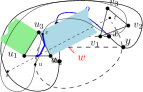
(b)

Figure 20: LABEL:sub@fig:add-deg-2 When adding triangles as in Lemma 11, $\mathcal{P}$ remains non-greedy. LABEL:sub@fig:confl-triang Conflicting triangles.

From now on, let triangles $\tau_{1},\dots,\tau_{n}$ form a triangulation of a simple hole-free polygon $\mathcal{P}$, and let $T$ be its corresponding dual binary tree. For simplicity we use $\tau_{i}$ to refer both to a triangle in $\mathcal{P}$ and its dual node in $T$.

Definition 12 (Projection of an edge).

For three non-collinear points $u_{1},u_{2},u_{3}$, let $\textnormal{proj}_{u_{1}}(u_{2}u_{3})$ denote the set of points covered by shifting $u_{2}u_{3}$ orthogonally to itself and away from $u_{1}$ (blue in Fig. 20b).

Definition 13 (Conflicting triangles).

Let $\tau_{i}=\triangle_{u_{1}u_{2}u_{3}}$ and $\tau_{j}=\triangle_{v_{1}v_{2}v_{3}}$ be two triangles such that the two edges dual to $u_{1}u_{2}$ and $v_{1}v_{2}$ are on the $\tau_{i}$-$\tau_{j}$ path in $T$. We call $\tau_{i}$, $\tau_{j}$ conflicting, if $\textnormal{proj}_{u_{1}}(u_{2}u_{3})\cup\textnormal{proj}_{u_{2}}(u_{1}u_{3})$ contains an interior point of $\tau_{j}$.

Lemma 12.

Let $T^{\prime}\subset T$ be a subtree of $T$ and let $\mathcal{P}^{\prime}$ be the corresponding simple polygon dual to $T^{\prime}$. Then $\mathcal{P}^{\prime}$ is a GRR if and only if no two triangles $\tau,\tau^{\prime}$ in $\mathcal{P}^{\prime}$ are conflicting.

Proof.

Assume there are two conflicting triangles $\tau_{i}=\triangle_{u_{1}u_{2}u_{3}},\tau_{j}=\triangle_{v_{1}v_{2}v_{3}}$ in $T^{\prime}$. Let $\mathcal{P}^{\prime\prime}$ denote the polygon defined by the $\tau_{i}$-$\tau_{j}$ path in $T^{\prime}$ and assume that the two edges dual to $u_{1}u_{2}$ and $v_{1}v_{2}$ are on the $\tau_{i}$-$\tau_{j}$ path. Since $\tau_{i}$ and $\tau_{j}$ are conflicting, there is, without loss of generality, a point $p$ on $u_{2}u_{3}$ such that $\textnormal{ray}_{u_{2}u_{3}}(p)$ intersects an edge of $\tau_{j}$. Hence, $\mathcal{P}^{\prime\prime}$ is not greedy. Moreover, $\mathcal{P}^{\prime}$ is obtained from $\mathcal{P}^{\prime\prime}$ by adding triangles. Thus Lemma 11 implies that $\mathcal{P}^{\prime}$ cannot be greedy.

Conversely, assume $\mathcal{P}^{\prime}$ is not greedy. There exists an outer edge $uv$ of $\mathcal{P}^{\prime}$ and a point $x$ in the interior of $uv$ such that $\textnormal{ray}_{uv}(x)$ crosses another boundary edge of $\mathcal{P}^{\prime}$ in a point $y$. Let $\tau_{x},\tau_{y}$ be the triangles with $x\in\tau_{x}$ and $y\in\tau_{y}$. Then $\tau_{x}$ and $\tau_{y}$ are conflicting. ∎

By Lemma 12, the decompositions of $\mathcal{P}$ in $k$ GRRs correspond bijectively to the multicuts $E^{\prime}$ of $T$ with $|E^{\prime}|=k-1$ where the terminal pairs are the pairs of conflicting triangles.

We now use the 2-approximation for Minimum Multicut on trees [11] to give a $(2-1/\operatorname{OPT})$-approximation for the minimum GRR decomposition of $\mathcal{P}$. Let $E^{\prime}$ be a 2-approximation of Minimum Multicut in $T$ with respect to the pairs of conflicting triangles. By the above observation the minimum multicut for $T$ has size $\operatorname{OPT}-1$, hence $|E^{\prime}|\leq 2\operatorname{OPT}-2$, which in turn yields a decomposition into $2\operatorname{OPT}-1$ regions. Thus the approximation guarantee is $2-1/\operatorname{OPT}$. We summarize this in Theorem 5.

Theorem 5.

There is a polynomial-time $(2-1/\operatorname{OPT})$-approximation for minimum GRR decomposition of triangulated simple polygons.

6 Conclusions

Motivated by a geographic routing protocol for dense wireless sensor networks proposed by Tan and Kermarrec [22], we further studied the problem of finding minimum GRR decompositions of polygons. We considered the special case of decomposing plane straight-line drawings of graphs, which correspond to infinitely thin polygons. For this case, we could apply insights gained from the study of self-approaching and increasing-chord drawings by the graph drawing community.

We extended the result of Tan and Kermarrec [22] for polygonal regions with holes by showing that partitioning a plane graph drawing into a minimum number of increasing-chord components is -hard. We then considered plane drawings of trees and showed how to model the decomposition problem using Minimum Multicut, which provided a polynomial-time 2-approximation. We solved the partitioning problem for trees optimally in polynomial time using dynamic programming. Finally, using insights gained from the decomposition of graph drawings, we gave a polynomial-time 2-approximation for decomposing triangulated polygons along their chords.

Open questions

For the -hard problem of decomposing plane drawings of graphs into the minimum number of GRRs, it is interesting to find approximation algorithms.

For decomposing polygons, many problems remain open. For example, one could investigate whether minimum decomposition is -hard for simple polygons for different types of allowed partition types. Is finding the optimum solution hard for partitioning triangulations as in Section 5? Is the minimum GRR decomposition problem hard if we allow cutting the polygon at any diagonal? Is it hard if arbitrary polygonal cuts are allowed, i.e., the partition can use Steiner points? Finally, are there approximations for partitioning polygons with and without holes into GRRs?

Acknowledgements

The second author thanks Jie Gao for pointing him to the topic of GRR decompositions.

References

- [1] S. Alamdari, T. M. Chan, E. Grant, A. Lubiw, and V. Pathak. Self-approaching graphs. In W. Didimo and M. Patrignani, editors, GD 2012, volume 7704 of LNCS, pages 260–271. Springer, 2013.
- [2] P. Bose, P. Morin, I. Stojmenović, and J. Urrutia. Routing with guaranteed delivery in ad hoc wireless networks. Wireless Networks, 7(6):609–616, 2001.
- [3] G. Calinescu, C. G. Fernandes, and B. Reed. Multicuts in unweighted graphs and digraphs with bounded degree and bounded tree-width. J. Algorithms, 48(2):333–359, 2003.
- [4] B. Chazelle and D. Dobkin. Optimal convex decompositions. In Computational Geometry, pages 63–133, 1985.
- [5] D. Chen and P. K. Varshney. A survey of void handling techniques for geographic routing in wireless networks. Commun. Surveys Tuts., 9(1):50–67, 2007.
- [6] M.-C. Costa, L. Létocart, and F. Roupin. A greedy algorithm for multicut and integral multiflow in rooted trees. Oper. Res. Lett., 31(1):21–27, 2003.
- [7] M.-C. Costa, L. Létocart, and F. Roupin. Minimal multicut and maximal integer multiflow: A survey. European Journal of Operational Research, 162(1):55 – 69, 2005.
- [8] A. Ćustić, B. Klinz, and G. J. Woeginger. Geometric versions of the three-dimensional assignment problem under general norms. Discrete Optimization, 18:38–55, 2015.
- [9] H. R. Dehkordi, F. Frati, and J. Gudmundsson. Increasing-chord graphs on point sets. J. Graph Algorithms Appl., 19(2):761–778, 2015.
- [10] Q. Fang, J. Gao, L. Guibas, V. de Silva, and L. Zhang. Glider: gradient landmark-based distributed routing for sensor networks. In INFOCOM 2005, pages 339–350. IEEE, 2005.
- [11] N. Garg, V. Vazirani, and M. Yannakakis. Primal-dual approximation algorithms for integral flow and multicut in trees. Algorithmica, 18(1):3–20, 1997.
- [12] C. Icking, R. Klein, and E. Langetepe. Self-approaching curves. Math. Proc. Camb. Phil. Soc., 125:441–453, 1999.
- [13] J. M. Keil. Decomposing a polygon into simpler components. SIAM Journal on Computing, 14(4):799–817, 1985.
- [14] D. E. Knuth and A. Raghunathan. The problem of compatible representatives. SIAM J. Discrete Math., 5(3):422–427, 1992.
- [15] E. Kranakis, H. Singh, and J. Urrutia. Compass routing on geometric networks. In Canadian Conference on Computational Geometry (CCCG’99), pages 51–54, 1999.
- [16] D. Lichtenstein. Planar formulae and their uses. SIAM Journal on Computing, 11(2):329–343, 1982.
- [17] M. Mauve, J. Widmer, and H. Hartenstein. A survey on position-based routing in mobile ad hoc networks. Network, IEEE, 15(6):30–39, 2001.
- [18] M. Nöllenburg, R. Prutkin, and I. Rutter. Partitioning graph drawings and triangulated simple polygons into greedily routable regions. In K. Elbassioni and K. Makino, editors, Algorithms and Computation (ISAAC’15), volume 9472, pages 637–649. Springer, 2015.
- [19] M. Nöllenburg, R. Prutkin, and I. Rutter. On self-approaching and increasing-chord drawings of 3-connected planar graphs. J. Comput. Geom., 7(1):47–69, 2016.
- [20] C. H. Papadimitriou and D. Ratajczak. On a conjecture related to geometric routing. Theoret. Comput. Sci., 344(1):3–14, 2005.
- [21] G. Tan, M. Bertier, and A.-M. Kermarrec. Convex partition of sensor networks and its use in virtual coordinate geographic routing. In INFOCOM 2009, pages 1746–1754. IEEE, 2009.
- [22] G. Tan and A.-M. Kermarrec. Greedy geographic routing in large-scale sensor networks: A minimum network decomposition approach. IEEE/ACM Transactions on Networking, 20(3):864–877, 2012.
- [23] X. Zhu, R. Sarkar, and J. Gao. Shape segmentation and applications in sensor networks. In INFOCOM 2007, pages 1838–1846. IEEE, 2007.