Asymptotic expressions for the hyperfine populations in the ground state of spin-1 condensates against a magnetic field

Abstract

Based on the perturbation theory up to the second order, analytical asymptotic expressions for the variation of the population of hyperfine component $\mu=0$ particles in the ground state of spin-1 condensates against a magnetic field $B$ has been derived. The ranges of $B$ in which the asymptotic expressions are applicable have been clarified via a comparison of the numerical results from the analytical expressions and from a diagonalization of the Hamiltonian in a complete spin-space. It was found that, For Rb, the two analytical expressions, one for a weak and the other one for a strong field, together cover the whole range of $B$ from 0 to infinite. For Na, the analytical expressions are valid only if $B$ is very weak or sufficiently strong.

.0.1 1, Introduction

The spinor condensates, as tunable systems with active spin-degrees of freedom, are rich in physics and promising in application. Since the pioneering experiment on spin-1 condensates ste the study of these systems becomes a hot topic.yka ; sta In general, in the study of spin-$f$ condensates, an important observable is the population of the particles lying in a given hyperfine-component $\mu=-f$ to $f$. These quantities are popularly measured in various experiments and are a key to relate experimental results to theories.ste ; dms ; hsc ; msc ; tku Hence, the theoretical study of these populations is desirable.

Let the hyperfine density of $\mu=0$ component in the ground state (g.s.) of spin-1 condensates be denoted as $\bar{\rho}_{0}$. When a magnetic field $B$ is applied, the variation of $\bar{\rho}_{0}$ as a function of $B$ is studied in this paper. A many-body theory, instead of the mean-field theory, is used so that the spin-degrees of freedom are treated rigorously. The emphasis is placed on the asymptotic behaviors of $\bar{\rho}_{0}$ when $B\rightarrow 0$ and $\rightarrow\infty$. Based on the second order perturbation theory analytical asymptotic expressions for $\bar{\rho}_{0}$ are derived. Numerical results from a diagonalization of the Hamiltonian are also obtained to compare with the results from the asymptotic expressions. In this way the effective ranges of $B$ wherein the asymptotic expressions are applicable are clarified. Thus, within the effective ranges, $\bar{\rho}_{0}$ can be quantitatively and accurately known, and in general the variation of $\bar{\rho}_{0}$ as a function of $B$ can be qualitatively understood.

.0.2 2, Hamiltonian in the spin-space

We consider $N$ spin-1 cold atoms trapped by an isotropic potential and subjected to a magnetic field. For spin-1 atoms the dipole-dipole interaction is extremely weak, and thus its effect on the coupling between the spatial- and spin-modes can be neglected (the quasi-spin-orbit coupling is not considered here). Let the total interaction $\hat{V}=\hat{V}_{0}+\hat{V}_{2}$, $\hat{V}_{0}=c_{0}\sum_{i<j}\delta(\mathbf{r}_{i}-\mathbf{r}_{j})$ and $\hat{V}_{2}=c_{2}\sum_{i<j}\delta(\mathbf{r}_{i}-\mathbf{r}_{j})\ \mathbf{f}_{i}\cdot\mathbf{f}_{j}$ where $\mathbf{f}_{i}$ is the spin-operator of the $i$-th particle.tlh ; ckl It was found that $|c_{2}/c_{0}|=0.0046$ for ⁸⁷Rb and 0.031 for ²³Na. Thus the spin-dependent force is nearly two order weaker than the central (spin-independent) force. Therefore, the spin-modes are much easier to get excited. Accordingly, the lowest lying levels would avoid spatial excitations but be dominated by spin-modes. With this in mind, it is assumed that the g.s. does not contain spatially excited modes, and all the particles fall into the same spatial state which is most advantageous to binding. This is the basic assumption of this paper.

The Hamiltonian $\hat{H}$ is

$$\hat{H}=\hat{H}_{0}+\hat{V}+q\Sigma_{i}f_{iz}^{2}$$ (1)

where $\hat{H}_{0}=\sum_{i}(-\frac{\hbar^{2}}{2m}\nabla_{i}^{2}+U(\mathbf{r}_{i}))$ includes the kinetic and trap energies, Since the Hamiltonian conserves the total magnetization $M$, the linear Zeeman term has been neglected. The third term at the right of eq.(1) is for the quadratic Zeeman energy, where $q$ is proportional to $B^{2}$.

When $B=0$, not only $M$, the total spin $S$ is also conserved. It has been proved that, for a spin-1 $N-body$ system, the all-symmetric spin-state with a pair of good quantum numbers $(S,M)$ is unique, where $N-S$ must be even.ka Let the total spin-state be denoted as $\vartheta_{SM}$. The set $\{\vartheta_{SM}\}$ form a complete set for all-symmetric spin-states. Thus, under the above basic assumption, the g.s. can be written in the form asbao3

$$\Phi_{\mathrm{gs}}=\Pi_{i}\phi(\mathbf{r}_{i})\vartheta_{S_{g}M}$$ (2)

where $\phi(\mathbf{r}_{i})$ is the common spatial state for all the particles, $S_{g}=N$ for Rb, and $S_{g}=M$ or ($M+1$) for Na if $N-M$ is even or (odd). In what follows $M\geq 0$ and $N-M$ being even are assumed for convenience.

When $B\neq 0$, $S$ is not conserved but $M$ is. Hence, different $\vartheta_{SM}$ having the same $M$ but distinct in $S$ are mixed up, and the g.s. can be in general written as

$$\Phi_{\mathrm{gs}}=\Pi_{i}\phi(\mathbf{r}_{i})\sum_{S}C_{S}\vartheta_{SM}\equiv\Pi_{i}\phi(\mathbf{r}_{i})\Theta_{gs}$$ (3)

Since the spatial degrees of freedom are considered as being frozen, the Schrödinger equation can be projected into the spin-space as

$$\int d\mathfrak{R}\Pi_{i}\phi^{\ast}(\mathbf{r}_{i})(H-E)\Psi=0$$ (4)

where the integration covers all the spatial degrees of freedom. Making use of the fact that $\sum_{i<j}\mathbf{f}_{i}\cdot\mathbf{f}_{j}=\frac{1}{2}\overset{\wedge}{S}^{2}-N$, where $\overset{\wedge}{S}$ is the operator of the total spin, the above equation becomes

$$(H^{\prime}-E^{\prime})\Theta_{gs}=0$$ (5)

Where $H^{\prime}=H_{0}^{\prime}+H_{1}^{\prime}$, $H_{0}^{\prime}=\frac{1}{2}Xc_{2}\overset{\wedge}{S}^{2}$, $H_{1}^{\prime}=q\Sigma_{i}f_{iz}^{2}$, $E^{\prime}=E-N\overset{\_}{h}-\frac{N(N-1)}{2}Xc_{0}+NXc_{2}$, $X\equiv\int d\mathbf{r}|\phi|^{4}$, and $\overset{\_}{h}=\langle\phi|-\frac{\hbar^{2}}{2m}\nabla_{i}^{2}+U(\mathbf{r}_{i})|\phi\rangle$. In what follows we work simply in the spin-space with the Hamiltonian $H^{\prime}$.

.0.3 3, Asymptotic behavior of the hyperfine density when $B\rightarrow 0$

When $B\rightarrow 0$, $H_{1}^{\prime}$ can be treated as a perturbation. Since $\vartheta_{SM}$ is an eigenstate of $H_{0}^{\prime}$ and the set $\{\vartheta_{SM}\}$ is complete, the perturbative states can be expanded in terms of $\{\vartheta_{SM}\}$. A crucial point is the calculation of the matrix element $\langle\vartheta_{S^{\prime}M}|H_{1}^{\prime}|\vartheta_{SM}\rangle\equiv Q_{S^{\prime}S}$. Making use of the fractional percentage coefficients by which the spin-state of a single particle can be extracted from $\vartheta_{SM}$,bao1 the general expression of $Q_{S^{\prime}S}$ can be obtained as given in eq.(2) to (7) of ref.bao2 . It turns out that $Q_{S^{\prime}S}$ can be nonzero only if $S^{\prime}=S$ or $S\pm 2$.

For Rb with $c_{2}<0$, the unperturbed g.s. in the spin-space is $\vartheta_{NM}$. Due to the limited choices of $S$ and $S^{\prime}$, the perturbative state up to the second order is

$$\Theta_{gs}\approx\vartheta_{NM}+\beta^{\prime}\vartheta_{N-2,M}+\beta\frac{Q_{N-4,N-2}}{Xc_{2}(4N-6)}\vartheta_{N-4,M}$$ (6)

where $\beta^{\prime}=\beta(1+\frac{Q_{N-2,N-2}-Q_{N,N}}{Xc_{2}(2N-1)})$, $\beta=\frac{Q_{N-2,N}}{Xc_{2}(2N-1)}$. From the general expression of $Q_{S^{\prime}S}$,

$$Q_{N,N}=q(M^{2}+N^{2}-N)/(2N-1),$$ (7)

$$Q_{N-2,N}=\frac{q}{2N-1}\left[\frac{2((N-1)^{2}-M^{2})(N^{2}-M^{2})}{(2N-3)}\right]^{\frac{1}{2}}$$ (8)

$$Q_{N-2,N-2}$$ (9)

$$= \frac{q[M^{2}(2N+3)+2N^{3}-7N^{2}+5N-2]}{(2N-1)(2N-5)}$$

and $Q_{N-4,N}=0$.

On the other hand, for any total spin-state, the operator $\Sigma_{i}f_{iz}^{2}$ is equivalent to $N-\overset{\wedge}{N_{0}}$, where $\overset{\wedge}{N_{0}}$ is the operator for the number of $\mu=0$ particles. Thus we have

$$\frac{\langle\Theta_{gs}|H_{1}^{\prime}|\Theta_{gs}\rangle}{q\langle\Theta_{gs}|\Theta_{gs}\rangle}=N-\frac{\langle\Theta_{gs}|\overset{\wedge}{N_{0}}|\Theta_{gs}\rangle}{\langle\Theta_{gs}|\Theta_{gs}\rangle}\equiv N-N\bar{\rho}_{0}$$ (10)

Inserting eq.(6) into (10), and making use of eq.(7) to (9), we have the hyperfine density with $\mu=0$ as

$$\bar{\rho}_{0} \approx (N^{2}-M^{2})/[N(2N-1)]$$

$$-\frac{1}{qN}(2\beta^{\prime}Q_{N-2,N}+(\beta^{\prime})^{2}(Q_{N-2,N-2}-Q_{NN}))$$

where the terms higher than $q^{2}$ are excluded. The first term is the $q\rightarrow 0$ limit of $\bar{\rho}_{0}$ for Rb and is denoted as $(\bar{\rho}_{0})_{q=0}$, which has been found before as given in eq.(18) of the ref.bao2 . Thus eq.(.0.3) is a generalization of the previous finding for magnetic field zero to nonzero. It turns out that $(N^{2}-M^{2})/[N(2N-1)]=(C_{1,0;N-1,M}^{N,M})^{2}$, where the Clebsch-Gordan coefficient is introduced. This is because, when $q=0$, the total spin of the g.s. $S_{g}=N$. Thus, each particle must couple to a $(N-1)-$body system with total spin $N-1$. Thus the probability of each single particle in $\mu=0$ is given by the above square.

It is notable that $(\bar{\rho}_{0})_{q=0}$ is irrelevant to dynamics but depends decisively on $M$. In particular, $(\bar{\rho}_{0})_{q=0}$ is close to 1/2 when $M$ is small, and is close to zero when $M\approx N$. Note that, for the frame upon it $M$ is defined, $M\approx 0$ implies that $S_{g}$ is lying close to the X-Y plane and therefore nearly half of the particles are in $\mu=0$. While the case $M\approx N$ implies that $S_{g}$ is lying close to the Z-axis and therefore the number of $\mu=0$ particles should be small. Note that the second term at the right of eq.(.0.3) is positive (because $\beta$ is negative when $c_{2}<0$). Thus, starting from $(\bar{\rho}_{0})_{q=0}$, $\bar{\rho}_{0}$ keeps increasing with $B$. This is natural because the g.s. would do its best to increase the number of $\mu=0$ particles so as to reduce the quadratic Zeeman energy.

For Na with $c_{2}>0$, the unperturbed g.s. is $\vartheta_{MM}$. The related matrix elements of $H_{1}^{\prime}$ are

$$Q_{MM}=q(2MN+2N+M)/(2M+3)$$ (12)

$$Q_{M+2,M}=\frac{2q}{2M+3}[\frac{(M+1)(N-M)(N+M+3)}{2M+5}]^{\frac{1}{2}}$$ (13)

$$Q_{M+2,M+2} = \frac{q}{(2M+3)(2M+7)}$$

$$[M^{2}(4N+2)+M(10N-5)+10N-6]$$

The perturbative state up to the second order is

$$\Theta_{gs}\approx\vartheta_{MM}+\gamma^{\prime}\vartheta_{M+2,M}-\gamma\frac{Q_{M+4,M+2}}{Xc_{2}(4M+10)}\vartheta_{M+4,M}$$ (15)

where $\gamma^{\prime}=\gamma(1+\frac{Q_{M+2,M+2}-Q_{MM}}{Xc_{2}(2N-1)})$, $\gamma=-\frac{Q_{M+2,M}}{Xc_{2}(2M+3)}$.

Inserting eq.(15) into eq.(10), we have

$$\bar{\rho}_{0} \approx (N-M)/[N(2M+3)]-\frac{1}{qN}(2\gamma^{\prime}Q_{M+2,M}$$ (16)

$$+(\gamma^{\prime})^{2}(Q_{M+2,M+2}-Q_{MM}))$$

where the terms higher than $q^{2}$ are excluded.. The first term is $(\bar{\rho}_{0})_{q=0}$ for Na. This form was first found in 2000 in the ref.tlh2 ; mko and also in bao2 derived in a different way later. Thus eq.(16) is a generalization of the previous finding from $B$ zero to nonzero. When $M=0$ the g.s. is in a pure polar phase and every particle is in a singlet pair. In this case the first term becomes 1/3 as stated in ref.sta ; bao2 and in the Theorem I of ref.tasa13 . Since the square of the Clebsch-Gordan coefficient for the singlet pair $(C_{1,\mu;1,-\mu}^{00})^{2}=1/3$, the probability of the particle in $\mu$ is therefore 1/3. This is the physical background of this value. When $M$ increases even a little from zero, the first term at the right of eq.(16) will decrease remarkably from 1/3 (say, when $M$ increases from 0 to $2$, $(\bar{\rho}_{0})_{q=0}$ decreases from 1/3 to $\sim 1/7$). This remarkable decrease arises from the factor $2M+3$ in the denominator. It implies that the appearance of a few polarized particles among the big group of singlet pairs could cause serious effect. Thus, for the case with $c_{2}>0$, the sensitivity against $M$ when $M$ is small is notable. Starting from $(\bar{\rho}_{0})_{q=0}$, $\bar{\rho}_{0}$ keeps increasing with $B$ (because $\gamma$ is negative) as in the previous case.

.0.4 4, Asymptotic behavior of the hyperfine density when $B\rightarrow\infty$

When $B\rightarrow\infty$, $H_{0}^{\prime}$, rather than $H_{1}^{\prime}$, can be treated as a perturbation. Since the Fock-state $|N_{1},N_{0},N_{-1}\rangle$, in which $N_{\mu}$ particles are in the $\mu$-component, is an eigenstate of $H_{1}^{\prime}$, the perturbative states can be expanded in terms of them. Since $N_{\pm 1}=(N-N_{0}\pm M)/2$, the Fock-state can be simply denoted as $|N_{0}\rangle$ when $M$ is fixed. Let $\langle N_{0}^{\prime}|H_{0}^{\prime}|N_{0}\rangle\equiv P_{N_{0}^{\prime}N_{0}}$. Making use of the formula, say, given in eq.(A5) of ref.ml , we have

$$P_{N_{0}N_{0}}=\frac{Xc_{2}}{2}(M^{2}+N+N_{0}+2NN_{0}-2N_{0}^{2})$$ (17)

$$P_{N_{0}-2,N_{0}}=\frac{Xc_{2}}{2}[N_{0}(N_{0}-1)((N-N_{0}+2)^{2}-M^{2})]^{\frac{1}{2}}$$ (18)

$$P_{N_{0}+2,N_{0}}=\frac{Xc_{2}}{2}[(N_{0}+1)(N_{0}+2)((N-N_{0})^{2}-M^{2})]^{\frac{1}{2}}$$ (19)

Otherwise, $P_{N_{0}^{\prime}N_{0}}=0$.

Note that, when $c_{2}\rightarrow 0$, the number of $\mu=0$ particles in the g.s. will be maximized so as to minimize the Zeeman energy. Thus, under the conservation of $M$, the leading term of $\Theta_{gs}$ should be $|N-M\rangle$. Accordingly, the perturbative state up to the second order is

$$\Theta_{gs}\approx |N-M\rangle+\delta^{\prime}|N-M-2\rangle$$ (20)

$$+ \delta\frac{P_{N-M-4,N-M-2}}{4q}|N-M-4\rangle$$

where $\delta^{\prime}=\delta(1+\frac{P_{N-M-2,N-M-2}-P_{N-M,N-M}}{2q})$, $\delta=\frac{P_{N-M-2,N-M}}{2q}$.

Inserting $\Theta_{gs}$ into eq.(10), we have

$$\bar{\rho}_{0}\approx\frac{N-M}{N}-\frac{2}{N}(\delta^{\prime})^{2}$$ (21)

where higher order terms have been neglected. This formula holds for both Rb and Na. Since the second term at the right of eq.(21) is negative, the first term appears as the upper bound.

.0.5 5, Applicability of the asymptotic expressions for c${}_{2}<0$

In order to clarify the applicability of the asymptotic expression, we have to find out the exact solutions of $H^{\prime}$. It is reminded that the set of eigenstates of $H_{0}^{\prime}$, $\{\vartheta_{SM}\}$, is complete for all the symmetric spin-states, therefore they can serve as the basis functions for the diagonalization of $H^{\prime}$ in the spin-space. The related matrix element $\langle\vartheta_{S^{\prime}M}|H^{\prime}|\vartheta_{SM}\rangle=\delta_{S^{\prime}S}\frac{Xc_{2}}{2}S(S+1)+Q_{S^{\prime}S}$, where $Q_{S^{\prime}S}$ is given in the ref.bao2 , and $X\equiv\int d\mathbf{r}|\phi|^{4}$ depends on the interaction and the trap. To obtain numerical results, $U(\mathbf{r})=\frac{1}{2}m\omega^{2}r^{2}$ is assumed. Note that $X$ does not appear in the leading terms of all the asymptotic expressions, and we consider only the cases with a large $N$. Thus, it is reasonable to evaluate $X$ under the Thomas-Fermi approximation (TFA). For details, we refer the reader to ref.TF . After the diagonalization one can extract $\bar{\rho}_{0}$ from the eigenstates of $H^{\prime}$ as given in eq.(9) of ref.bao2 . Numerical results of $\bar{\rho}_{0}$ from the asymptotic expressions and from the diagonalization are compared below.

It turns out that, when $q=0$ and $q=\infty$, the resultant $\bar{\rho}_{0}$ from the perturbative approach and from the exact diagonalization of $H^{\prime}$ are identical. Furthermore, we always have $(\bar{\rho}_{0})_{q\rightarrow\infty}\geq\bar{\rho}_{0}\geq$ $(\bar{\rho}_{0})_{q=0}$ (where the equality holds only if $M=N$). Thus the variation of $\bar{\rho}_{0}$ versus $q$ is strictly restricted in a domain which can be known in advance, and $\bar{\rho}_{0}$ keeps increasing with $q$ inside the domain. The increasing arises because the g.s. would like to have more $\mu=0$ particles to reduce the quadratic Zeeman energy. We introduce a ratio $\alpha$ so that $M=\alpha N$. For Rb, we know from eq. (.0.3) and (21) that $(\bar{\rho}_{0})_{q=0}\approx\frac{1}{2}(1-\alpha^{2})$ and $(\bar{\rho}_{0})_{q\rightarrow\infty}=1-\alpha$. In what follows, $\alpha$ is given at 1/2 and 0.001, respectively. Accordingly, the magnetization is half and nearly zero. The case $\alpha\simeq 1$ (corresponding to a nearly full magnetization) is trivial because both the lower and upper bounds are close to zero, and nearly no $\mu=0$ particles will emerge.

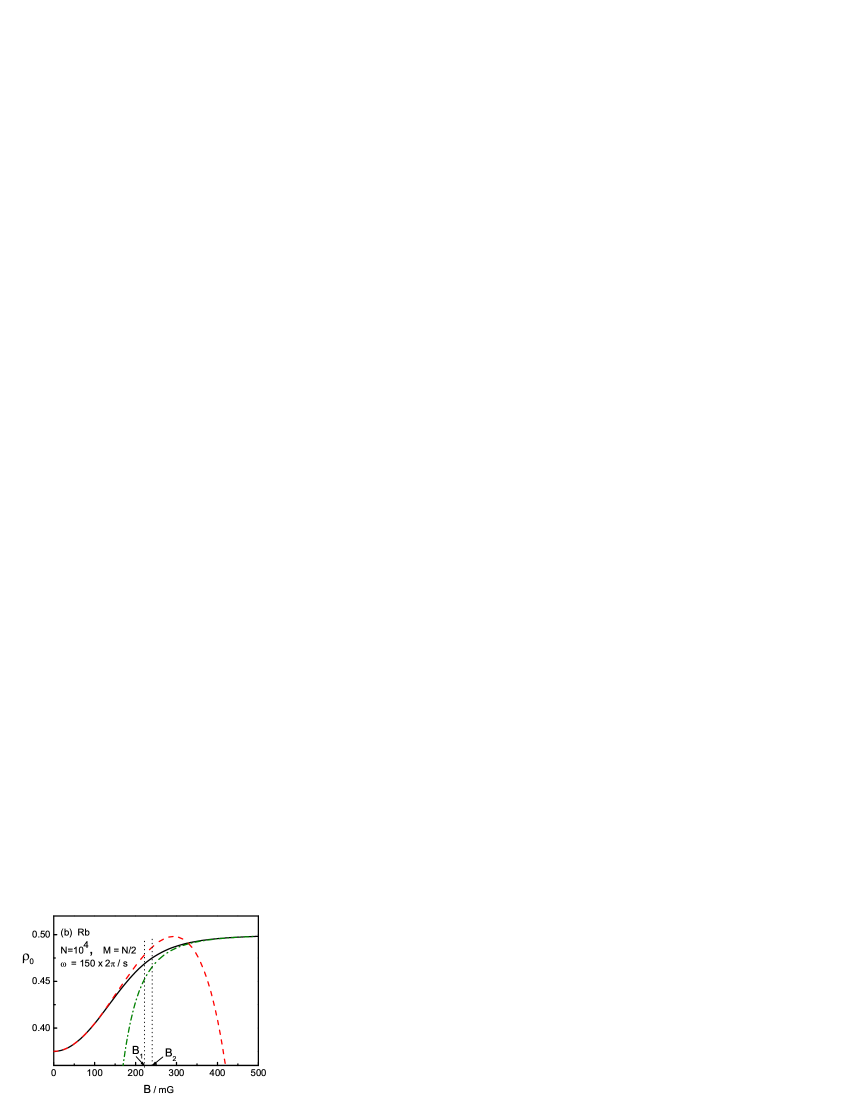
Figure 1: (Color online) The three densities $(\bar{\rho}_{0})_{exact}$ (solid), $(\bar{\rho}_{0})_{asym,1}$(dash), and $(\bar{\rho}_{0})_{asym,2}$(dash-dot) of Rb versus $B/mG$. $M=N/2$. The trap is assumed to be $\frac{1}{2}m\omega^{2}r^{2}$. $(\bar{\rho}_{0})_{asym,1}$ is effective (close to $(\bar{\rho}_{0})_{exact}$) when $B$ lies in $(0,B_{1})$, while $(\bar{\rho}_{0})_{asym,2}$ is effective in $(B_{2},\infty)$. $B_{1}$ and $B_{2}$ are marked by two vertical dotted lines. Note that the upper panel has a larger $\omega$, and accordingly the curves shift to the right. It implies that, for a stronger trap, a stronger $B$ is needed to raise up the number of $\mu=0$ particles.

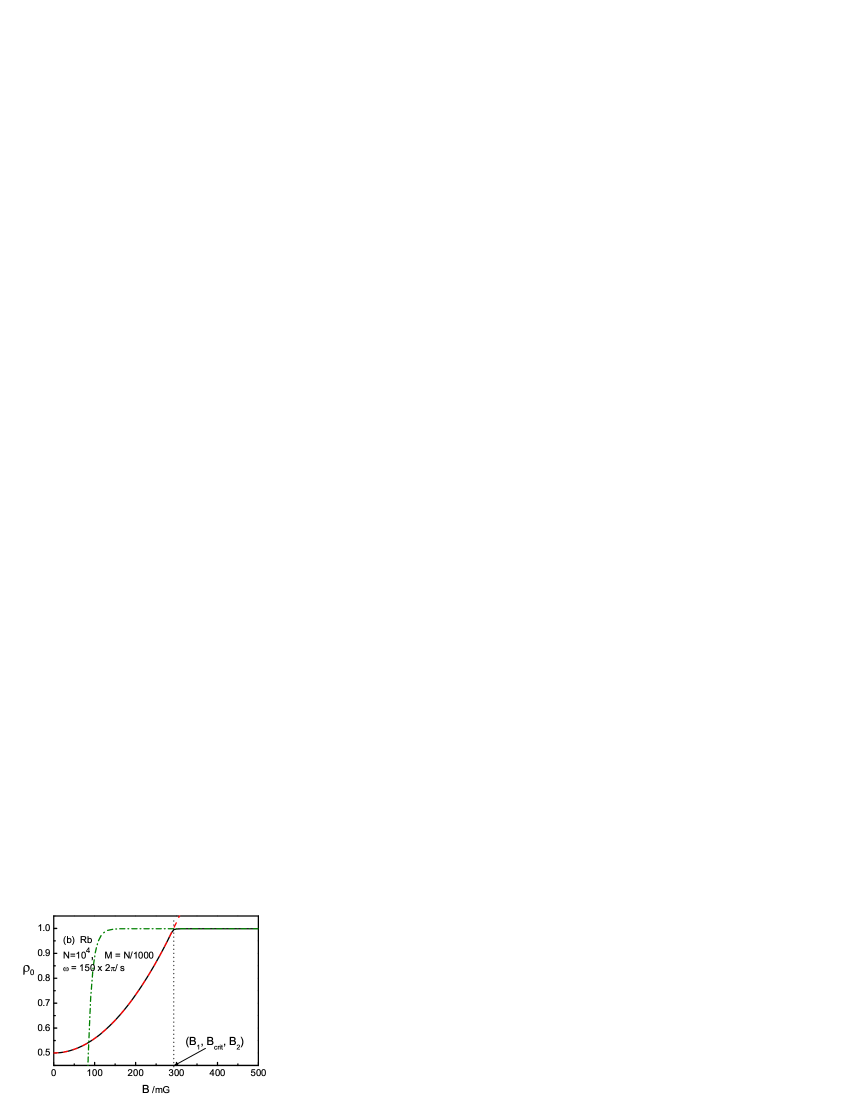
Figure 2: (Color online) The same as Fig.1 but with $M=N/1000$. There is a sharp change in $(\bar{\rho}_{0})_{exact}$ at $B_{crit}$ marked by a vertical dotted line. $B_{1}\approx$ $B_{crit}\approx B_{2}$ is found.

Examples of the variation of the densities $\bar{\rho}_{0}$ versus $B$ with $N=10000$ and $\alpha=1/2$ (0.001) is shown in Fig.1 (Fig.2). Accordingly, $\bar{\rho}_{0}$ is increasing from 3/8 to 1/2 and from 1/2 to 0.999, respectively. To measure the deviation between the exact and asymptotic results, we define $x_{i}=|(\bar{\rho}_{0})_{exact}-(\bar{\rho}_{0})_{asym,i}|$ where $(\bar{\rho}_{0})_{exact}$ denotes that the density is from the exact diagonalization of $H^{\prime}$, while $(\bar{\rho}_{0})_{asym,i}$ is from the asymptotic expression eq.(.0.3) (if $i=1$) or from eq.(21) (if $i=2$). To give a quantitative description, we define $B_{1}$ at which $x_{1}=0.01$, and $B_{2}$ at which $x_{2}=0.01$. We found that, when $B<B_{1}$ ($>B_{2}$), $x_{1}$ ($x_{2}$) is even smaller than 0.01. Thus, we can say that the effective range of $B$, in which eq.(.0.3) is very close to be exact, is [$0,B_{1}$], and the effective range for eq.(21) is [$B_{2},\infty$].

The case with a half-magnetization ($\alpha=1/2$) is shown in Fig.1. In Fig.1a $(B_{1},B_{2})=(343mG$, $361mG)$. Thus, the effective range for $(\bar{\rho}_{0})_{asym,1}$ and the effective range for $(\bar{\rho}_{0})_{asym,2}$ together cover nearly the whole range of $B$. It is emphasized that both the lower and upper bounds depend only on $\alpha$ but not on $N$ and/or $\omega$. Therefore, when $N$ and/or $\omega$ are changed, the variation of the curves is limited because they are fixed at their two ends and they must keep increasing with $B$. Nonetheless, $B_{1}$ and $B_{2}$ will therefore be changed. For an example, the $\omega$ in 1a is two times the $\omega$ in 1b. Accordingly, the curves in 1a as a whole shift to the right. Numerical examples of $(B_{1},B_{2})$ with different $N$ and $\omega$ are given in Table I.

Table 1: $B_{1}$ and $B_{2}$ in $mG$ for Rb with $\alpha\equiv M/N=1/2$. Two cases of $N$ and three cases of $\omega$ are considered, where $\omega_{o}=300\times 2\pi/s$.

		N=10000	N=20000
$\omega_{o}/2$		226, 238	260, 274
$\omega_{o}$		343, 361	393, 414
$2\omega_{o}$		520, 548	596, 629

We know from the Table that $B_{2}$ is close to $B_{1}$ in general, and therefore the asymptotic expressions are nearly valid in the whole range of $B$. They will both be larger when $N$ and/or $\omega$ are larger, or vice versa. Nonetheless, they are more sensitive to $\omega$ rather than $N$. When $\omega$ is larger, the spin-texture of the g.s. would have a stronger ability to resist the field. This causes a shift of the curves to the right.

The case with a nearly zero magnetization ($\alpha=0.001$) is shown in Fig.2. It was found in 2a (2b) that both $B_{1}$ and $B_{2}$ are very close to a critical point $B_{crit}=446mG$ (292$mG$) at which $(\bar{\rho}_{0})_{exact}$ undergoes a sharp change. The change is so sharp that the second order derivative of $(\bar{\rho}_{0})_{exact}$ against $B$ tends to $\infty$ when $N\rightarrow\infty$. Obviously, this implies a phase transition. It turns out that the two curves $(\bar{\rho}_{0})_{asym,i}$ and $(\bar{\rho}_{0})_{asym,i}$ intercept when $B\sim B_{crit}$, and this is a common feature for the g.s. with $c_{2}<0$ and with a nearly zero-magnetization. Thus the effective ranges for the two asymptotic expressions together cover the whole range of $B$, and the two expressions together provide a perfect description of $\bar{\rho}_{0}$. Numerical examples of $B_{crit}$ are given in Table II.

Table 2: $B_{crit}$ in $mG$ for Rb with $\alpha=0.001$. In this case $B_{1}\approx B_{2}\approx B_{crit}$. $\omega_{o}$ is referred to Table I.

		N=10000	N=20000
$\omega_{o}/2$		292	337
$\omega_{o}$		446	514
$2\omega_{o}$		678	778

Similar to the previous case, a larger $N$ and/or a larger $\omega$ lead to a larger $B_{crit}$, and the vice versa. When $B>B_{crit}$, the curve of $(\bar{\rho}_{0})_{exact}$ becomes horizontal. It implies that, after the phase transition, the system arrives at its eventual status (this status is described by the Fock-state $|M,N-M,0\rangle$, where $N-M$ particles have $\mu=0$ while the rest have $\mu=1$). In this status the number of $\mu=0$ particles has been maximized, and therefore no more change is allowed when $B$ increases further. Note that the sharp change will become ambiguous when $M$ is larger. Comparing 2b with 2a, it is clear that $B_{crit}$ will shift to the right when $\omega$ increases.

.0.6 6, Applicability of the asymptotic expressions for c${}_{2}>0$

Let us predict two features of spin-1 condensates with $c_{2}>0$.

(i) When $B=0$, the total spin-state of the g.s. has $S=M$ and is denoted as $\vartheta_{MM}\propto\overset{\char 126\relax}{\mathcal{S}}\chi_{1}^{M}(\chi\chi)_{0}^{(N-M)/2}$, where $\chi_{1}$ denotes the spin-state of a single particle with $\mu=1$, $(\chi\chi)_{0}$ denotes a singlet pair, and $\overset{\char 126\relax}{\mathcal{S}}$ is a symmetrizer. If there are another forms, they are identical due to the uniqueness of the eigenstate.ka Thus, the g.s. is a mixture of a group of polarized particles together with a group of singlet pairs. Obviously, the $M$ particles in the first group are stable against $B$, while the $N-M$ particles in the second group are not. Note that every singlet pair is situated under the same environment, thus they have similar ability to resist $B$. It is possible that all the pairs might begin to be broken when $B$ increases and exceeds a certain value, and therefore a sharp change of the spin-texture will occur.

(ii) In general, the stability of the g.s. depends on the gap (the energy difference between the g.s. and the first excited state). When $B=0$ the g.s. has $S=M$ while the first excited state has $S=M+2$, therefore the gap is $\propto(4M+6)$ for $c_{2}>0$, whereas this factor would be $(4N-2)$ for $c_{2}<0$. Therefore, the gap for Na is much smaller than that for Rb when $\alpha$ is small. In this case, the g.s. of Na is highly unstable and the feature of the system will depend on $\alpha$ sensitively. In other words, the singlet pairs will become more fragile when $\alpha\rightarrow 0$.

We found from eq.(16) and eq.(21) that the lower and upper bounds are$\ (\bar{\rho}_{0})_{q=0}=(1-\alpha)/(2\alpha N+3)$ and $(\bar{\rho}_{0})_{q\rightarrow\infty}=1-\alpha$, respectively, and they are identical to the numerical values from the exact diagonalization of $H^{\prime}$. In particular, when $\alpha=0$, $(\bar{\rho}_{0})_{q=0}=1/3$ and $(\bar{\rho}_{0})_{q=\infty}=1$. Note that, when $\alpha=0$, every particle is in a singlet pair. Recalled that the Clebsch-Gordan coefficient $C_{1,\mu;1,-\mu}^{0,0}=(-1)^{1-\mu}1/\sqrt{3}$. Therefore, when a particle is in a singlet pair, the probability in $\mu$ is 1/3. This leads to $(\bar{\rho}_{0})_{q=0}=1/3$. On the other hand, $(\bar{\rho}_{0})_{q=\infty}=1$ implies obviously that all particles are in the $\mu=0$ component. This results from the minimization of the quadratic Zeeman energy.

For any $\alpha$, we have $(\bar{\rho}_{0})_{q=0}\leq\bar{\rho}_{0}\leq(\bar{\rho}_{0})_{q\rightarrow\infty}$, and $\bar{\rho}_{0}$ keeps increasing in between as before. Note that the $(\bar{\rho}_{0})_{q\rightarrow\infty}$ of the two species Rb and Na are the same, but the $(\bar{\rho}_{0})_{q=0}$ of Na is always lower than that of Rb. Thus, when $q$ varies, the $\bar{\rho}_{0}$ of Na varies in a broader domain. Note that the $\alpha-$sensitivity of $(\bar{\rho}_{0})_{q=0}$ is embodied in the factor $2\alpha N$ which appears in the denominator (Say, when $N=10000$, and $\alpha=0$ and $0.001$, respectively, $(\bar{\rho}_{0})_{q=0}=1/3$ and $1/23$. Thus a small change in $\alpha$ leads to a big change in $(\bar{\rho}_{0})_{q=0}$).

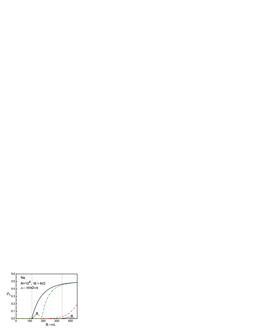
Figure 3: (Color online) The three densities of Na versus $B/mG$. Refer to Fig.1.

For the case of half-magnetization ($\alpha=1/2$), the variation of $\bar{\rho}_{0}$ versus $B$ is shown in Fig.3 where $N=10000$ and $\omega=\omega_{o}\equiv 300\times 2\pi/s$. There is a sudden uprising in $(\bar{\rho}_{0})_{exact}$ as mentioned in point (i) taking place when $B=B_{crit}=114mG$. It turns out that $(\bar{\rho}_{0})_{asym,1}$ is identical or extremely close to $(\bar{\rho}_{0})_{exact}$ when $B\leq B_{crit}$, but deviates from $(\bar{\rho}_{0})_{exact}$ rapidly when $B>B_{crit}$. Therefore, in this case, we have $B_{1}\approx B_{crit}$ and therefore the effective range for $(\bar{\rho}_{0})_{asym,1}\$is $(0,B_{crit})$. Numerical examples of $B_{crit}$ and $B_{2}$ (the latter is much larger) are shown in Table III.

Table 3: $B_{1}\approx B_{crit}$ and $B_{2}$ in $mG$ for Na with $\alpha=1/2$. Refer to Table I.

		N=10000	N=20000
$\omega_{o}/2$		77, 226	90, 259
$\omega_{o}$		118, 342	136, 393
$2\omega_{o}$		176, 519	204, 595

Thus, both $B_{1}$ and $B_{2}$ will be larger when $N$ and/or $\omega$ are larger as before, or the vice versa. In fact, $B_{crit}$ measures the ability of the singlet pairs to keep themselves unbroken against $B$. It is obvious that this ability will become stronger when the trap is stronger ($\omega$ is larger). It is interesting to see that this ability will also become a little stronger when $N$ increases.

Recalled that the $B_{crit}$ for Rb marks the maximization of the $\mu=0$ particles. Now, the $B_{crit}$ for Na marks the solidity of the singlet pairs. This explains why the curve is horizontal when $B>B_{crit}$ for Rb, and when $B<B_{crit}$ for Na. In the latter case the pairs are kept unbroken and the spin-texture remains unchanged.

The case of nearly zero-magnetization ($\alpha=0.001$) is shown in Fig.4. It is shown in Fig.4a (for $B\leq 1mG$) that $(\bar{\rho}_{0})_{exact}$ increases very fast when $B$ is ranged from $0.2mG$ to $1mG$. One can define a critical strength $B_{crit}$ at which the second order derivative of $(\bar{\rho}_{0})_{exact}$ against $B$ arrives at its maximum. In Fig.4a $B_{crit}=0.26mG$. It is further found that the effective range of $B$ for $(\bar{\rho}_{0})_{asym,1}$ to be applicable is from 0 to $B_{1}=0.29mG$. Thus $B_{1}$ is again very close to $B_{crit}$. Once $B>B_{crit}$, although both $(\bar{\rho}_{0})_{asym,1}$ and $(\bar{\rho}_{0})_{exact}$ increase sharply, they deviate more and more from each other. For the case that $\alpha$ is very small, the effective range for $(\bar{\rho}_{0})_{asym,1}$ is very narrow. As an example, if $\alpha$ is further reduced from 0.001 to zero, $B_{1}$ would be reduced from 0.29mG to 0.04mG, and $B_{crit}$ is reduced from 0.26mG to zero. Thus, the singlet pairs will become very fragile when $\alpha\rightarrow 0$ as predicted in (ii).

How $B_{1}$ and $B_{2}$ are affected by $N$ and $\omega$ is shown in Table IV.

Table IV, $B_{1}$ and $B_{2}$ in $mG$ for Na with $\alpha=0.001$. Refer to Table I.

Table 4: $B_{1}$ and $B_{2}$ in $mG$ for Na with $\alpha=0.001$. Refer to Table I.

		10000	20000
$\omega_{o}/2$		0.17, 163	0.18, 187
$\omega_{o}$		0.26, 248	0.27, 282
$2\omega_{o}$		0.39, 375	0.41, 428

.0.7 7, Summary

When $B$ tends to zero and infinite, the asymptotic forms of the hyperfine density $\bar{\rho}_{0}$ against $B$ denoted as $(\bar{\rho}_{0})_{asym,1}$ and $(\bar{\rho}_{0})_{asym,2}$, respectively, has been obtained analytically based on the second order perturbation theory. Numerical calculation via an exact diagonalization of $H^{\prime}$ for the density denoted as $(\bar{\rho}_{0})_{exact}$ has been performed to clarify the effective ranges of $B$ wherein the asymptotic forms $(\bar{\rho}_{0})_{asym,i}$ are applicable. The two ranges for $i=1$ and $i=2$, respectively, are specified as $(0,B_{1}$) and $(B_{2},\infty)$. It turns out that the two limits $(\bar{\rho}_{0})_{q=0}$ and $(\bar{\rho}_{0})_{q=\infty}$ given by the analytical expressions are identical to those from the exact diagonalization of $H^{\prime}$. They together provide the lower and upper bounds for $\bar{\rho}_{0}$, and $\bar{\rho}_{0}$ is monotonously increasing with $q$ between them. Thus, in any case, we can have a rough impression on $\bar{\rho}_{0}$.

For Rb, both $B_{1}$ and $B_{2}$ are in the order of $10^{2}mG$, and they are close to each other when the parameters vary in a broad domain that are accessed frequently in experiments. Thus, $\bar{\rho}_{0}$ can be accurately known when $B$ lies inside one of the ranges, or can be roughly known when $B$ lies between $B_{1}$ and $B_{2}$. In particular, when $\alpha\equiv M/N$ is small, (i) A critical strength $B_{crit}$ is found which marks the realization of the eventual status, in which the number of $\mu=0$ particles is maximized. (ii) $B_{1}$, $B_{2}$, and $B_{crit}$ are close to each other, and therefore the two asymptotic forms together cover nearly the whole range.

For Na, a critical strength $B_{crit}$ is also found but has another implication, it marks the sudden breaking of the singlet pairs. At a weak field $\bar{\rho}_{0}$ is highly sensitive to $\alpha$ when $\alpha$ is small. Note that, when $\alpha$ increases from zero, a few polarized particles will emerge among the numerous singlet pairs and lead to a remarkable increase of $B_{crit}$. It implies that the singlet pairs will become more solid thereby. Thus the emergence of a few specific particles can cause serious effect, similar to the serious effect of a few impurity appearing in well organized crystal structure. The underlying physics deserves to be further studied.

In general, when the spin-texture undergoes a sharp change (this appears as a phase transition when $N\rightarrow\infty$), $(\bar{\rho}_{0})_{exact}$ is able to describe this change. However, the perturbation theory fails to describe such a sharp change. This is the main shortcoming of the perturbation theory and is the reason that $(\bar{\rho}_{0})_{asym,i}$ will begin to deviate sharply from $(\bar{\rho}_{0})_{exact}$ when $q$ is close to the critical points.

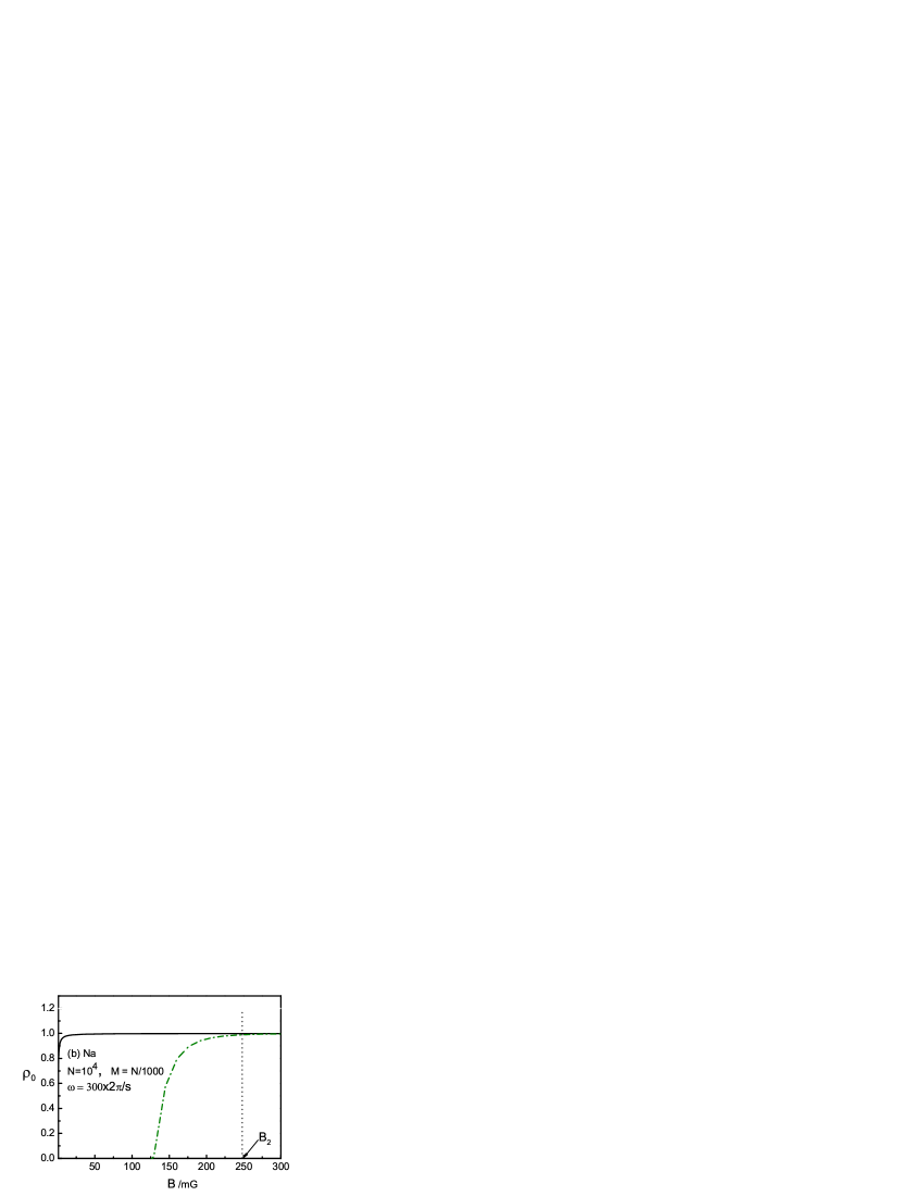
Figure 4: (Color online) The same as Fig.3 but with $M=N/1000$. The range of $B$ is $0\rightarrow 1mG$ in 3a where $B_{1}$ is marked, whereas $B$ is $1\rightarrow 300mG$ in 4b where $B_{2}$ is marked. $(\bar{\rho}_{0})_{asym,2}$ does not appear in 4a, while $(\bar{\rho}_{0})_{asym,1}$ does not appear in 4b.