Semiclassical solutions of generalized Wheeler-DeWitt cosmology

Abstract

We consider an extension of WDW minisuperpace cosmology with additional interaction terms that preserve the linear structure of the theory. General perturbative methods are developed and applied to known semiclassical solutions for a closed Universe filled with a massless scalar. The exact Feynman propagator of the free theory is derived by means of a conformal transformation in minisuperspace. As an example, a stochastic interaction term is considered and first order perturbative corrections are computed. It is argued that such an interaction can be used to describe the interaction of the cosmological background with the microscopic d.o.f. of the gravitational field. A Helmoltz-like equation is considered for the case of interactions that do not depend on the internal time and the corresponding Green’s kernel is obtained exactly.The possibility of linking this approach to fundamental theories of Quantum Gravity is investigated.

I Introduction

The Wheeler-DeWitt (WDW) equation represents the starting point of the canonical quantization program, also known as geometrodynamics. It was originally derived by applying Dirac’s quantization scheme to Einstein’s theory of gravity, formulated in Arnowitt-Deser-Misner (ADM) variables. It has the peculiar form of a timeless Schrödinger equation, whose solutions are functions defined on the space of three-dimensional geometries

$$H\psi=0\leavevmode\nobreak\ .$$ (1)

The equation is a constraint imposed on physical states, encoding the invariance of the theory under reparametrization of the time variable. Together with the (spatial) diffeomorphism constraint, it expresses the principle of general covariance at the quantum level. This approach has however several limitations that prevented it from being accepted as a fully satisfactory theory of Quantum Gravity in its original formulation. Nonetheless, some of the issues it raises, as for instance the problem of time (i.e. the lack of a universal parameter used to describe the evolution of the gravitational field), are actually problems encountered by all fundamental (nonperturbative) approaches to quantum gravity. Others stem instead from the dubious mathematical structure of the theory. Among the most essential ones in the latter category we mention the factor ordering problem in the Hamiltonian constraint and the construction of a physical Hilbert space.

Despite its limitations, WDW was proved to be a valuable instrument in cases where the number of degrees of freedom is restricted a priori, i.e. in minisuperspace and midisuperspace models. In particular, its application to cosmological settings has been extremely useful to gain insight into some of the deep questions raised by a quantum theory of the gravitational field, such as the problem of time Halliwell and the occurrence of stable macroscopic branches for the state of the Universe (as in the consistent histories approach Craig-Singh:2010 ).

One of the fundamental aspects of WDW is its linearity. This is indeed a consequence of the Dirac quantization procedure and a property of any first-quantized theory. One can nonetheless find in the literature several proposals for non-linear extensions of the geometrodynamics equation. They are in general motivated by an interpretation of $\psi$ in Eq. (1) as a field operator (rather than a function) defined on the space of geometries. This idea has been applied to Cosmology and found concrete realization in the old baby Universes approach Giddings:1988 . More recently, a model motivated by Group Field Theory (GFT) (see Ref. Oriti:2014 for a recent outline) has been proposed in Ref. Calcagni:2012 that retains the same spirit, taking Loop Quantum Cosmology (LQC) AshtekarBojowald2003 as a starting point.

It is worthwhile stressing that the WDW theory can be recovered in the continuum limit (see Ref. Ashtekar:2006 for details) from a more fundamental theory such as LQC. In this sense it can be interpreted as an effective theory of Quantum Cosmology, valid at scales such that the fundamentally discrete structure of spacetime cannot be probed. Therefore WDW, far from being of mere historical relevance, is rather to be considered as an important tool to extract predictions from cosmological models when a continuum, semiclassical behaviour is to be expected.

In what follows we consider as a starting point the Hamiltonian constraint of LQC, leading to the free evolution of the Universe, as discussed in the GFT-inspired model  Calcagni:2012 . Non-linear terms are allowed, which can be interpreted as interactions between disconnected homogeneous components of an isotropic Universe (scattering processes describe topology change). Instead of resorting to a third quantized formalism built on minisuperspace models, we follow a rather conservative approach which does not postulate the existence of Universes disconnected from ours. We therefore only take into account linear modifications of the theory, so as to guarantee that the superposition principle remains satisfied. Hence these extra terms can be interpreted as self-interactions of the Universe, as well as violations of the Hamiltonian constraint.

We aim at studying the dynamics in a regime such that the free LQC dynamics (given by finite difference equation) can be approximately described in terms of differential equations. In this regime, the dynamics is given by a modified WDW equation. The additional interactions should be such that deviations from the Friedmann equation are small, and will therefore be treated as small perturbations.

We consider a closed Friedmann-Lemaître-Robertson-Walker (FLRW) Universe, for which semiclassical solutions are known explicitly Kiefer:1988 . Corrections to the solutions arising from the extra linear interactions are obtained perturbatively. Of particular interest is the case in which the perturbation is represented by white noise. In fact, this could be a way to model the effect of the discrete structure underlying spacetime on the evolution of the macroscopically relevant degrees of freedom. It should therefore be possible to make contact, at least qualitatively, between the usual quantum cosmology and the GFT cosmology, according to which the dynamics of the Universe is that of a condensate of elementary spacetime constituents. Considering a white noise term amounts to treating the vacuum fluctuations of the gravitational field as a stochastic process, an approach motivated by an analogy with Stochastic Electrodynamics (SED) Lamb-shift-SED ; de1983stochastic ; Lamb-shift-spontaneous-emission-SED ; QM-SED . This will be done is Section VI. The analogy with SED has of course its limitations, since in the case at hand there is no knowledge about the dynamics of the vacuum, which should instead come from a full theory of Quantum Gravity. In spite of this limitation, the methods developed here are fully general, so as to allow for a perturbative analysis of the solutions of the linearly modified WDW equation for any possible form of the additional interactions.

In the present work we restrict to a closed Universe, for which wave packet solutions were constructed in Ref. Kiefer:1988 . In the same work, it was shown that it is possible to construct a quantum state whose evolution mimics a solution of the classical Friedmann equation, and is given by a quantum superposition of two Gaussian wave packets (one for each of the two phases of the Universe, expanding and contracting) centered on the classical trajectory. We build on the results of Ref. Kiefer:1988 , considering the new interaction term as a perturbation, and thus determining the corrections to the motion of the wave packets.

The rest of the paper is organized as follows: In Sec. II, we show how our model is motivated by LQC and GFT inspired cosmology Calcagni:2012 in the continuum limit (large volumes). In Sec. III, we review the construction of the wave packet solutions done in Ref. Kiefer:1988 . These solutions will be used in the subsequent sections as the unperturbed states describing the evolution of a semiclassical Universe. In Sec. IV, using the scalar field to define an internal time, we develop a framework for time-independent perturbation theory. The inverse of the Helmoltz operator corresponding to the free theory is computed exactly and turns out to depend on a real parameter, linked to the choice of the boundary conditions at the singularity. An analogue of Ehrenfest’s theorem for the evolution equation of the expectation values of observables is then given. In Sec. V, the Feynman propagator of the WDW free field operator is evaluated exactly. This is accomplished by using a conformal map in minisuperspace, which reduces the problem to that of finding the Klein-Gordon propagator in a planar region with a boundary. In Sec. VI, we consider the case in which the additional interaction is given by white noise. In Sec. VII, we discuss the rôle of the Noether charge and the choice of the inner product. Finally, we review our results and their physical implications in Sec. VIII.

II From the LQC free theory to WDW

Let us briefly show how the WDW equation is recovered from the Hamiltonian constraint of LQC following Ref. Ashtekar:2006  . For our purposes it is convenient to consider a massless scalar field $\phi$, minimally coupled to the gravitational field. This choice has the advantage of allowing for a straightforward deparametrization of the theory, thus defining a clock. The Hamiltonian constraint has the general structure Ashtekar:2006 ; Calcagni:2012

$$\hat{\mathcal{K}}\psi(\nu,\phi)\equiv-B(\nu)\left(\Theta+\partial_{\phi}^{2}\right)\psi(\nu,\phi)=0\leavevmode\nobreak\ ,$$ (2)

where $\psi$ is a wave function on configuration space, $\Theta$ is a finite difference operator acting on the gravitational sector in the kinetic Hilbert space of the theory $\mathcal{H}^{\rm g}_{\rm kin}$, and $\nu$ denotes the generic eigenvalue of the volume operator. The discreteness introduced by the LQC formulation does not affect the matter sector, which is still the same as in the continuum WDW quantum theory. The gravitational sector of the Hamiltonian constraint operator of LQC in “improved dynamics” , reads

$$-B(\nu)\Theta\,\psi(\nu,\phi)\equiv A(\nu)\psi(\nu+\nu_{0},\phi)+C(\nu)\psi(\nu,\phi)+D(\nu)\psi(\nu-\nu_{0},\phi)\leavevmode\nobreak\ ,$$ (3)

where the finite increment $\nu_{0}$ represents an elementary volume unit and $A,B,C,D$ are functions which depend on the chosen quantization scheme. In order to guarantee that $\Theta$ is symmetric in $\nu$, the coefficients must satisfy the $D(\nu)=A(\nu-\nu_{0})$ condition Calcagni:2012 ; it holds in both the $k=0$ and the $k=1$ case.

It is a general result of LQC that WDW can be recovered in the continuum (i.e. large volume) limit Ashtekar:2007 . In particular, it was shown in Ref. Ashtekar:2006 that for $k=1$ one recovers the Hamiltonian constraint of Ref. Kiefer:1988 . In fact it turns out that $\Theta$ can be expressed as the sum of the operator ($\Theta_{0}$) relative to the $k=0$ case and a $\phi$-independent potential term (i.e. diagonal in the $\nu$ basis) as

$$\Theta=\Theta_{0}+\frac{\pi Gl_{0}^{2}\gamma^{2}}{3K^{4/3}}|\nu|^{4/3}\leavevmode\nobreak\ .$$ (4)

In the above expression $K=\frac{2\sqrt{2}}{3\sqrt{3\sqrt{3}}}$, $\gamma$ is the Barbero-Immirzi parameter of Loop Quantum Gravity (LQG), $G$ the gravitational constant and $l_{0}$ is the cube root of the fiducial volume of the fiducial cell on the spatial manifold in the $k=1$ model. The latter can be formally sent to zero in order to recover the $k=0$ case.

Restricting to wave functions $\psi(\nu)$ which are smooth and slowly varying in $\nu$, we obtain the WDW limit of the Hamiltonian constraint

$$\Theta_{0}\psi(\nu,\phi)=-12\pi G(\nu\partial_{\nu})^{2}\psi(\nu,\phi)\leavevmode\nobreak\ ,$$ (5)

which is exactly the same constraint one obtains in WDW theory. Thus, LQC naturally recovers the factor ordering (also called factor ordering, in the sense that the quantum constraint operator is of the form $G^{AB}\nabla_{A}\nabla_{B}$, where $G^{AB}$ is the inverse WDW metric and $\nabla_{A}$ denotes the covariant derivative associated with $G_{AB}$) which was obtained in Ref. Halliwell under the requirement of field reparametrization invariance of the minisuperspace path-integral. Since $\nu$ represents a proper volume, it is proportional to the volume of a comoving cell with linear dimension equal to the scale factor $a$

$$\nu\propto a^{3}\leavevmode\nobreak\ .$$ (6)

Introducing the variable $\alpha=\log a$, we rewrite the constraint operator $\hat{\mathcal{K}}$ as

$$\hat{\mathcal{K}}=e^{-3\alpha}\left(\frac{\partial^{2}}{\partial\alpha^{2}}-\frac{\partial^{2}}{\partial\phi^{2}}-e^{4\alpha}\right)\leavevmode\nobreak\ .$$ (7)

Let us consider a modified dynamical equation of the form

$$\hat{\mathcal{K}}\psi(\nu,\phi)+\sum_{\nu^{\prime}}\int\mbox{d}\phi^{\prime}\;g(\nu,\nu^{\prime};\phi,\phi^{\prime})\psi(\nu^{\prime},\phi^{\prime})=0\leavevmode\nobreak\ ,$$ (8)

which, in the continuum limit $\nu\gg\nu_{0}$, leads to

$$\left(\frac{\partial^{2}}{\partial\alpha^{2}}-\frac{\partial^{2}}{\partial\phi^{2}}-e^{4\alpha}\right)\psi=-e^{3\alpha}\int\mbox{d}\alpha^{\prime}\,\mbox{d}\phi^{\prime}\;\left.{\mbox{d}\nu\over\mbox{d}\alpha}\right|_{\alpha^{\prime}}g\psi\leavevmode\nobreak\ .$$ (9)

We will assume that the interaction $g$ is local in minisuperspace, i.e. $g(\nu,\nu^{\prime};\phi,\phi^{\prime})=g(\nu,\phi)\delta(\nu-\nu{\prime})\delta(\phi-\phi^{\prime})$. Given the properties of the Dirac delta function

$$\delta(\nu-\nu^{\prime})=\frac{\delta(\alpha-\alpha^{\prime})}{\left.{\mbox{d}\nu\over\mbox{d}\alpha}\right|_{\alpha^{\prime}}}\leavevmode\nobreak\ ,$$ (10)

Equation (9) reduces to a Klein-Gordon equation with space and time dependent potential $e^{3\alpha}g(\alpha,\phi)$; note that $g$ is kept completely general.

Since the interaction term represented by the r.h.s. of Eq.(9) is unknown, we cannot determine an exact solution of the equation without resorting to a case by case analysis. However, since the solutions of the WDW equation in the absence of a potential are known explicitly, we will adopt a perturbative approach. The method we develop is fully general and can thus be applied for any possible choice of the function $g$.

We formally expand the wave function and the WDW operator in terms of a dimensionless parameter $\lambda$ (that serves book-keeping purposes and will be eventually set equal to $1$).

$$\psi=\psi^{(0)}+\lambda\psi^{(1)}+\dots\leavevmode\nobreak\ ,$$ (11)

$$\mbox{and}\ \ \hat{T}=\hat{T}_{0}+\lambda e^{3\alpha}\int g\leavevmode\nobreak\ ,$$ (12)

with the definitions

$$\hat{T}_{0}\equiv\left(\frac{\partial^{2}}{\partial\alpha^{2}}-\frac{\partial^{2}}{\partial\phi^{2}}-e^{4\alpha}\right).$$ (13)

We therefore have

$$\hat{T}_{0}\psi^{(0)} =0\leavevmode\nobreak\ ,$$ (14)

$$\hat{T}_{0}\psi^{(1)} =-e^{3\alpha}g\,\psi^{(0)}\leavevmode\nobreak\ .$$ (15)

The zero-th order term $\psi^{(0)}$ is a solution of the wave equation with an exponential potential, which was obtained in Ref. (Kiefer:1988, ) and will be reviewed in the next section. If we were able to invert $\hat{T}_{0}$, we would get the wave function corrected to first order. However, finding the Green’s function is not straightforward in this case as it would be for $k=0$ (where the kinetic operator is just the d’Alembertian, whose Green’s kernels are well known for all possible choices of boundary conditions). Moreover, as for the d’Alembertian, the Green’s kernel will depend on the boundary conditions. The problem of determining which set of boundary conditions is more appropriate depends on the physical situation we have in mind and will be dealt with in the next sections.

At this point, we would like to point out the relation between our approach and the model in Ref. Calcagni:2012 , where a third quantization perspective is assumed. The action on minisuperspace that was considered in Ref. Calcagni:2012 reads

$$S[\psi]=S_{\rm free}[\psi]+\sum_{n}\frac{\lambda_{n}}{n!}\sum_{\nu_{1}\dots\nu_{n}}\int\mbox{d}\phi_{1}\dots\mbox{d}\phi_{n}\;f^{(n)}(\nu_{i},\phi_{i})\prod_{j}\psi(\nu_{j},\phi_{j})\leavevmode\nobreak\ ,$$ (16)

where the first term gives the dynamics of the free theory, namely a homogeneous and isotropic gravitational background coupled to a massless scalar field

$$S_{\rm free}[\psi]=\sum_{\nu}\int\mbox{d}\phi\;\psi(\nu,\phi)\hat{\mathcal{K}}\psi(\nu,\phi)\leavevmode\nobreak\ ;$$ (17)

$\hat{\mathcal{K}}$ is the Hamiltonian constraint in LQC and the terms containing the functions $f^{(n)}$ represent additional interactions that violate the constraint. This is a toy model for Group Field Cosmology (Calcagni:2012, ), given by a GFT with group $G=U(1)$ and $\nu$ a Lie algebra element. The free dynamics depends on the specific LQC model adopted. However, the continuum limit should be the same regardless of the model considered and must give the WDW equation for the corresponding three-space topology. The WDW approach to quantum cosmology should therefore be interpreted as an effective theory, valid at scales such that the discreteness introduced by the polymer quantization cannot be probed. We will show that, even from this more limited perspective, the action Eq. (16) leads to novel effective theory of quantum cosmology that represent modifications of WDW.

It was hinted in Ref. Calcagni:2012 that the additional interactions could also be interpreted as interactions occurring between homogeneous patches of an inhomogeneous Universe. Another possible interpretation is that they actually represent interactions among different, separate, Universes. The latter turns out to be a natural option in the framework of third quantization (see Ref. Isham:1992 and references therein), which naturally allows for topology change.

We restrict our attention to the quadratic term, that can be interpreted as a self interaction of the Universe. This is in fact worth considering even without resorting to a third-quantized cosmology and can in principle be generalized to include non-locality in minisuperspace (this situation will not be dealt with in the present work).

III Analysis of the unperturbed case

We review here the construction of wave packet solutions for the cosmological background presented in Ref. Kiefer:1988 . The Wheeler-DeWitt equation for a homogeneous and isotropic Universe (compact spatial topology, $k=1$) with a massless scalar field is

$$\left(\frac{\partial^{2}}{\partial\alpha^{2}}-\frac{\partial^{2}}{\partial\phi^{2}}-e^{4\alpha}\right)\psi(\alpha,\phi)=0\leavevmode\nobreak\ .$$ (18)

We impose the boundary condition

$$\lim_{\alpha\to\infty}\psi(\alpha,\phi)=0\leavevmode\nobreak\ ,$$ (19)

necessary in order to reconstruct semiclassical states describing the dynamics of a closed Universe, since regions of minisuperspace corresponding to arbitrary large scale factors are not accessible.

Equation (19) can be solved by separation of variables

$$\psi_{k}(\alpha,\phi)=N_{k}\,C_{k}(\alpha)\varphi_{k}(\phi)\leavevmode\nobreak\ ,$$ (20)

leading to

$$\frac{\partial^{2}}{\partial\phi^{2}}\varphi_{k}+k^{2}\varphi_{k} =0\leavevmode\nobreak\ ,$$ (21)

$$\frac{\partial^{2}}{\partial\alpha^{2}}C_{k}-(e^{4\alpha}-k^{2})C_{k} =0\leavevmode\nobreak\ .$$ (22)

Note that $\psi_{k}(\alpha,\phi)$ stands for the solution of Eq. (18) and should not be confused with the Fourier transform of $\psi$, for which we will use instead the notation $\tilde{\psi}(\alpha,k)$. In Eq. (20) above, $N_{k}$ is a normalization factor that depends on $k$, whose value will be fixed later.

Let us proceed with the solutions of Eqs. (21), (22). Equation (21) yields complex exponentials as solutions

$$\varphi_{k}=e^{ik\phi}\leavevmode\nobreak\ ,$$ (23)

while Eq. (22) has the same form as the stationary Schrödinger equation for a non-relativistic particle in one dimension, with potential $V(\alpha)=e^{4\alpha}-k^{2}$ and zero energy. One then easily remarks that the particle is free for $\alpha\rightarrow-\infty$, whereas the potential barrier becomes infinitely steep as $\alpha$ takes increasingly large positive values. Given the imposed boundary condition, Eq. (22) admits as an exact solution the modified Bessel function of the second kind (also known as MacDonald function)

$$C_{k}(\alpha)=K_{ik/2}\left(\frac{e^{2\alpha}}{2}\right)\leavevmode\nobreak\ .$$ (24)

Wave packets are then constructed as linear superpositions of the (appropriately normalized) solutions

$$\psi(\alpha,\phi)=\int_{-\infty}^{\infty}\mbox{d}k\;\psi_{k}(\alpha,\phi)A(k)\leavevmode\nobreak\ ,$$ (25)

with an appropriately chosen amplitude $A(k)$. Since the $C_{k}(\alpha)$ are improper eigenfunctions of the (one-parameter family of) Hamitonian operator(s) in Eq. (22), they do not belong to the space of square integrable functions on the real line $L^{2}(\mathbb{R})$. However, it is still possible to define some sort of normalization by fixing the oscillation amplitude of the improper eigenfunctions for $\alpha\to-\infty$. For this purpose, we recall the WKB expansion of Eq. (24)

$$K_{ik/2}\left(\frac{e^{2\alpha}}{2}\right)=\frac{\sqrt{\pi}}{2}e^{-k\frac{\pi}{4}}(k^{2}-e^{4\alpha})^{-1/4}\cos\left(\frac{k}{2}\operatorname{arccosh}\frac{k}{e^{2\alpha}}-\frac{1}{2}\sqrt{k^{2}-e^{4\alpha}}-\frac{\pi}{4}\right)\leavevmode\nobreak\ ,$$ (26)

a very accurate approximation for large values of $k$. We therefore set

$$\psi_{k}(\alpha,\phi)=e^{k\frac{\pi}{4}}\sqrt{k}\;K_{ik/2}\left(\frac{e^{2\alpha}}{2}\right)e^{ik\phi}\leavevmode\nobreak\ ,$$ (27)

which for large enough values of $k$ gives elementary waves with the same amplitude to the left of the potential barrier. Note that for small $k$, the amplitude $A(k)$ will still exhibit dependence on $k$.

Let us assume a Gaussian profile for the amplitude $A(k)$ in Eq. (25)

$$A(k)=\frac{1}{\pi^{1/4}\sqrt{b}}e^{-\frac{(k-\overline{k})^{2}}{2b^{2}}}\leavevmode\nobreak\ ,$$ (28)

where $\overline{k}$ should be taken large enough so as to guarantee the normalization of the function $\psi_{k}(\alpha,\phi)$. One then finds that the solution has the profile shown in the Fig. 2. The solution represents a wave packet that starts propagating from a region where the potential vanishes (i.e. at the initial singularity) towards the potential barrier located approximately at $\alpha_{\overline{k}}=\frac{1}{2}\log\overline{k}$, from where it is reflected back. For such values of $\overline{k}$ the wave packet is practically completely reflected back from the barrier. The parameter $b$ gives a measure of the semiclassicality of the state, i.e. it accounts for how much it peaks on the classical trajectory. We remark that the peak of the wave packet follows closely the classical trajectory,

$$e^{2\alpha}={\bar{k}\over\cosh(2\phi)}\leavevmode\nobreak\ .$$ (29)

and refer the reader to Fig. 2.

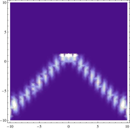
Figure 1: Absolute square of the “wave function” of the Universe corresponding to the choice of parameters $b=1$, $\overline{k}=10$. Lighter shades correspond to larger values of the wave function. During expansion and recollapse the evolution of the Universe can be seen as a freely propagating wave packet. From the plot it is also evident the reflection against the potential barrier at $\alpha_{\overline{k}}=\frac{1}{2}\log\overline{k}$, where the wave function exhibits a sharp peak.

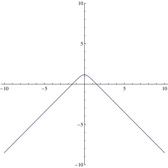
Figure 2: Classical trajectory of the Universe in minisuperspace. It is closely followed by the peak of semiclassical states, as we can see by comparison with Fig. 2.

IV Time independent perturbation potential

In the case in which the potential in the r.h.s of Eq. (9) does not depend on the scalar field (that we interpret as an internal time) we can resort to time-independent perturbation theory to calculate the corrections to the wave function. Namely, we consider the representation of the operator $\hat{T}_{0}$ defined in Eq. (13) in Fourier space, or equivalently its action on a monochromatic wave, so that we are lead to the Helmoltz equation in the presence of a potential

$$\left(\frac{\partial^{2}}{\partial\alpha^{2}}+k^{2}-e^{4\alpha}\right)\tilde{\psi}^{(0)}(\alpha,k)=0\leavevmode\nobreak\ ,$$ (30)

where the potential cannot be considered as a small perturbation with respect to the standard Helmoltz equation. In fact, reflection from an infinite potential barrier requires boundary conditions that are incompatible with those adopted in the free particle case. We therefore have to solve Eq. (30) exactly.

In order to compute the first perturbative corrections, we need to solve Eq. (15), which in Fourier space leads to

$$\left(\frac{\partial^{2}}{\partial\alpha^{2}}+k^{2}-e^{4\alpha}\right)\tilde{\psi}^{(1)}(\alpha,k)=U(\alpha)\tilde{\psi}^{(0)}(\alpha,k)\leavevmode\nobreak\ ,$$ (31)

upon defining $U(\alpha)=-e^{3\alpha}g(\alpha)$. Equation (31) is easily solved once the Green’s function of the Helmoltz operator on the l.h.s is known. The equation for the Green’s function is

$$\left(\frac{\partial^{2}}{\partial\alpha^{2}}+k^{2}-e^{4\alpha}\right)G^{k}(\alpha,\alpha^{\prime})=\delta(\alpha-\alpha^{\prime})\leavevmode\nobreak\ .$$ (32)

The homogeneous equation admits two linearly independent solutions, which we can use to form two distinct linear combinations that satisfy the boundary conditions at the two extrema of the interval of the real axis we are considering. The remaining free parameters are then fixed by requiring continuity of the function at $\alpha^{\prime}$ and the condition on the discontinuity of the first derivative at the same point.

Equation (30) has two linearly independent solutions $p(\alpha)$ and $h(\alpha)$ given by

$$p(\alpha)=K_{i\frac{k}{2}}\left(\frac{e^{2\alpha}}{2}\right)$$ (33)

and

$$h(\alpha)=I_{-i\frac{k}{2}}\left(\frac{e^{2\alpha}}{2}\right)+I_{i\frac{k}{2}}\left(\frac{e^{2\alpha}}{2}\right)\leavevmode\nobreak\ .$$ (34)

We thus make the following ansatz

$$G^{k}(\alpha,\alpha^{\prime})=\begin{cases}\gamma\;p(\alpha)&\alpha\geq\alpha^{\prime}\\ \delta\;h(\alpha)+\eta\;p(\alpha)&\alpha<\alpha^{\prime}\leavevmode\nobreak\ ,\end{cases}$$ (35)

and note that $G^{k}(\alpha,\alpha^{\prime})$ satisfies the boundary condition Eq. (19) by construction.

Since we do not know what is the boundary condition for $\alpha\to-\infty$, i.e. near the classical singularity, we will not be able to fix the values of all constants $\gamma,\delta,\eta$. We will therefore end up with a one-parameter family of Green’s functions.

The Green’s function must be continuous at the point $\alpha=\alpha^{\prime}$, hence

$$\gamma\;p(\alpha^{\prime})=\delta\;h(\alpha^{\prime})+\eta\;p(\alpha^{\prime})\leavevmode\nobreak\ .$$ (36)

Moreover, in order for its second derivative to be a Dirac delta functional, the following condition on the discontinuity of the first derivative must be satisfied

$$\gamma\;p^{\prime}(\alpha^{\prime})-\delta\;h^{\prime}(\alpha^{\prime})-\eta\;p^{\prime}(\alpha^{\prime})=1\leavevmode\nobreak\ .$$ (37)

Upon introducing a new constant $\Omega=\gamma-\eta$, we can rewrite Eqs. (36), (37) in the form of a Kramer’s system

$$\begin{cases}\Omega\;p(\alpha^{\prime})-\delta\;h(\alpha^{\prime})&=0\leavevmode\nobreak\ ,\\ \Omega\;p^{\prime}(\alpha^{\prime})-\delta\;h^{\prime}(\alpha^{\prime})&=1\leavevmode\nobreak\ ,\end{cases}$$

which admits a unique solution, given by

$$\Omega =-\frac{h(\alpha^{\prime})}{W(\alpha^{\prime})}\leavevmode\nobreak\ ,$$ (38)

$$\delta =-\frac{p(\alpha^{\prime})}{W(\alpha^{\prime})}\leavevmode\nobreak\ ,$$ (39)

where $W(\alpha^{\prime})=p(\alpha^{\prime})h^{\prime}(\alpha^{\prime})-h(\alpha^{\prime})p^{\prime}(\alpha^{\prime})$ is the Wronskian. Hence the ansatz (35) is rewritten as

$$G^{k,\eta}(\alpha,\alpha^{\prime})=\begin{cases}p(\alpha)\left(\eta-\frac{h(\alpha^{\prime})}{W(\alpha^{\prime})}\right)&\alpha\geq\alpha^{\prime}\\ -\frac{p(\alpha^{\prime})}{W(\alpha^{\prime})}\;h(\alpha)+\eta\;p(\alpha)&\alpha\leq\alpha^{\prime}\leavevmode\nobreak\ ,\end{cases}$$

where we have explicitly introduced the parameter $\eta$ in our notation for the Green’s function in order to stress its non-uniqueness. Note that the phase shift at $-\infty$ varies with $\eta$.

Hence the solution of Eq. (31) reads

$$\tilde{\psi}^{(1)}(\alpha,k)=\int\mbox{d}\alpha^{\prime}\;G^{k,\eta}(\alpha,\alpha^{\prime})U(\alpha^{\prime})\tilde{\psi}^{(0)}(\alpha,k)\leavevmode\nobreak\ .$$ (40)

The possibility of studying the perturbative corrections using a decomposition in monochromatic components is viable because of the validity of the superposition principle. This is in fact preserved by additional interactions of the type considered here, which violate the constraint while preserving the linearity of the wave equation. Note that in general, modifications of the scalar constraint in the WDW theory would be non-linear and non-local, as for instance within the proposal of Ref. Oriti:2010 , where classical geometrodynamics arises as the hydrodynamics limit of GFT. However, such non-linearities would spoil the superposition principle, hence making the analysis of the solutions much more involved.

The time dependence of the perturbative corrections is recovered by means of the inverse Fourier transform of Eq. (40)

$$\psi^{(1)}(\alpha,\phi)=\int\frac{\mbox{d}k}{2\pi}\;\tilde{\psi}^{(1)}(\alpha,k)e^{-ik\phi}\leavevmode\nobreak\ .$$ (41)

Expectation values of observables can be defined using the measure determined by the time component of the Noether current $j_{\phi}$ (whose definition will be given in Sec. VII) as

$$\langle f\rangle=\int\mbox{d}\alpha\;fj_{\phi}\leavevmode\nobreak\ .$$ (42)

Using the conservation of the Noether current we can then derive an analogue of Ehrenfest theorem, namely

$$\frac{\mbox{d}}{\mbox{d}\phi}\langle f\rangle=\int\mbox{d}\alpha\;\left(j_{\phi}\partial_{\phi}f+f\partial_{\phi}j_{\phi}\right)=\int\mbox{d}\alpha\;\left(j_{\phi}\partial_{\phi}f+f\partial_{\alpha}j_{\alpha}\right)\leavevmode\nobreak\ .$$ (43)

When the observable $f$ does not depend explicitly on the internal time $\phi$, the first term in the integrand vanishes. Considering for instance the scale factor $a=e^{\alpha}$ then, after integrating by parts, we get

$$\frac{\mbox{d}}{\mbox{d}\phi}\langle a\rangle=-\int\mbox{d}\alpha\;e^{\alpha}j_{\alpha}\leavevmode\nobreak\ .$$ (44)

In an analogous fashion, one can show that

$$\frac{\mbox{d}}{\mbox{d}\phi}\langle a^{2}\rangle=-2\int\mbox{d}\alpha\;e^{2\alpha}j_{\alpha}\leavevmode\nobreak\ .$$ (45)

Formulae (43) and (45), besides their simplicity, turn out quite handy for numerical computations, especially when dealing with time independent observables. In fact they can be used to compute time derivatives of the averaged observables without the need for a high resolution on the $\phi$ axis, i.e. they can be calculated using data on a single time-slice. Expectation values can therefore be propagated forwards or backwards in time by solving first order ordinary differential equations.

V First perturbative correction for time-dependent potentials

In the previous section we considered a time-independent perturbation, which can be dealt with using the Helmoltz equation. This is in general not possible when the perturbation depends on the internal time. In order to study the more general case we have to resort to different techniques to find the exact Green’s function of the operator $\hat{T}_{0}$. Since the potential $e^{4\alpha}$ breaks translational symmetry, Fourier analysis, which makes the determination of the propagator so straight-forward in the $k=0$ case (where the Hamiltonian constraint leads to the wave equation), is of no help.

Let us perform the following change of variables

$$X=\frac{1}{2}e^{2\alpha}\cosh(2\phi)\leavevmode\nobreak\ \leavevmode\nobreak\ ,\hskip 10.00002ptY=\frac{1}{2}e^{2\alpha}\sinh(2\phi)\leavevmode\nobreak\ ,$$ (46)

which represents a mapping of minisuperspace into the wedge $X>|Y|$. The minisuperspace interval (corresponding to DeWitt’s supermetric) can be expressed in the new coordinates as

$$\mbox{d}\phi^{2}-\mbox{d}\alpha^{2}=\frac{1}{X^{2}-Y^{2}}(\mbox{d}Y^{2}-\mbox{d}X^{2})\leavevmode\nobreak\ ,$$ (47)

with $(X^{2}-Y^{2})^{-1}$ the conformal factor. As an immediate consequence of conformal invariance, uniformly expanding (contracting) Universes are given by straight lines parallel to $X=Y$ ($X=-Y$) within the wedge. The “horizons” $X=-Y$ and $X=Y$ represent the initial and final singularity, respectively. It is worth pointing out that the classical trajectory Eq. (29) takes now the much simpler expression

$$\overline{k}=2X\leavevmode\nobreak\ ,$$ (48)

i.e. classical trajectories are represented by straight lines parallel to the $Y$ axis and with the extrema on the two singularities.

In the new coordinates $X,Y$ the operator $\hat{T}_{0}$ in Eq. (13) reads

$$\hat{T}_{0}=(X^{2}-Y^{2})(\partial_{X}^{2}-\partial_{Y}^{2}-4)\leavevmode\nobreak\ ,$$ (49)

which is, up to the inverse of the conformal factor, a Klein-Gordon operator with $m^{2}=4$. This is a first step towards a perturbative solution of Eq. (15), which we rewrite below for convenience of the reader in the form

$$\hat{T}_{0}\psi^{(1)}=U(\alpha,\phi)\psi^{(0)}\leavevmode\nobreak\ ,$$ (50)

where

$$U(\alpha,\phi)=-e^{3\alpha}g(\alpha,\phi)\leavevmode\nobreak\ .$$ (51)

Note that the above is the same equation as the one considered in the previous section, but we are now allowing for the interaction potential to depend also on $\phi$. Given Eq. (49), we recast Eq. (50) in the form that will be used for the applications of the next section, namely

$$(\partial_{X}^{2}-\partial_{Y}^{2}-4)\psi^{(1)}=\frac{U(X,Y)}{(X^{2}-Y^{2})}\psi^{(0)}\leavevmode\nobreak\ .$$ (52)

The formal solution to Eq. (52) is given by a convolution of the r.h.s with the Green’s function satisfying suitably chosen boundary conditions

$$\psi^{(1)}(X,Y)=\int\mbox{d}X^{\prime}\mbox{d}Y^{\prime}\;G(X,Y;X^{\prime},Y^{\prime})\frac{U(X^{\prime},Y^{\prime})}{(X^{\prime 2}-Y^{\prime 2})}\psi^{(0)}(X^{\prime},Y^{\prime})\leavevmode\nobreak\ .$$ (53)

The Green’s function of the Klein-Gordon operator in free space is well-known for any dimension $D$ (see e.g. Ref. Zhang ). In $D=2$ it is formally given by

$$G(X,Y;X^{\prime},Y^{\prime})=\int\frac{\mbox{d}^{2}k}{(2\pi)^{2}}\frac{e^{-i\left(k_{Y}(Y-Y^{\prime})-k_{X}(X-X^{\prime})\right)}}{\left(k_{Y}^{2}-k_{X}^{2}\right)-4}\leavevmode\nobreak\ ,$$ (54)

and satisfies the equation

$$(\partial_{X}^{2}-\partial_{Y}^{2}-4)G(X,Y;X^{\prime},Y^{\prime})=\delta(X-X^{\prime})\delta(Y-Y^{\prime})\leavevmode\nobreak\ .$$ (55)

Evaluating (54) explicitly using Feynman’s integration contour, which is a preferred choice in the context of a third quantization, we get disessa ; Zhang

$$G(X,Y;X^{\prime},Y^{\prime})=-\frac{1}{4}\theta(s)H_{0}^{(2)}(2\sqrt{s})-\frac{i}{2\pi}\theta(-s)K_{0}(2\sqrt{-s})\leavevmode\nobreak\ ,$$ (56)

where we introduced the notation $s=(Y-Y^{\prime})^{2}-(X-X^{\prime})^{2}$ for the interval. However, the present situation is distinguished from the free case, since there is a physical boundary represented by the edges of the wedge. The boundary conditions must be therefore appropriately discussed. A preferred choice is the one that leads to the Feynman boundary conditions in the physical coordinates $(\alpha,\phi)$. In the following, we will see the form that these conditions take in the new coordinate system, finding the transformation laws of the operators that annihilate progressive and regressive waves.

We begin by noticing that the generator of dilations in the $(X,Y)$ plane acts as a tangential derivative along the edges

$$X\partial_{X}+Y\partial_{Y}=\partial_{t}\leavevmode\nobreak\ .$$ (57)

Moreover on the upper edge $X=Y$ (corresponding to the big crunch) we have

$$\partial_{t}|_{X=Y}=\frac{1}{4}\left(\partial_{\alpha}+\partial_{\phi}\right)\leavevmode\nobreak\ ,$$ (58)

while on the lower edge (corresponding to the initial singularity) we have

$$\partial_{t}|_{X=-Y}=\frac{1}{4}\left(\partial_{\alpha}-\partial_{\phi}\right)\leavevmode\nobreak\ .$$ (59)

Therefore the boundary conditions

$$\partial_{t}|_{X=Y}G=\partial_{t}|_{X=-Y}G=0$$ (60)

are equivalent to the statement that the Green’s function is a positive (negative) frequency solution of the wave equation at the final (initial) singularity. This is in agreement with the Feynman prescription and with the fact that the potential $e^{\alpha}$ vanishes at the singularity $\alpha\to-\infty$.

There is a striking analogy with the classical electrostatics problem of determining the potential generated by a point charge inside a wedge formed by two conducting plates (in fact it is well-known that the electric field is normal to the surface of a conductor, so that the tangential derivative of the potential vanishes). The similarity goes beyond the boundary conditions and holds also at the level of the dynamical equation. In fact, after performing a Wick rotation $Y\to-i\,Y$ Eq. (55) becomes the Laplace equation with a constant mass term, while the operator $\partial_{t}$ defined in Eq. (57) keeps its form.

After performing the Wick rotation the problem can be solved with the method of images. Given a source (charge) at point $P_{0}=(r^{\prime},\theta^{\prime})$, three image charges as in Fig. 4 are needed to guarantee that the boundary conditions are met. The Euclidean Green’s function as a function of the point $Q=(r,\theta)$ and source $P_{0}$ (hence $m=2$) is shown to be given by

$$G(r,\theta,r^{\prime},\theta^{\prime})=\frac{1}{2\pi}\left(K_{0}(m\,\overline{P_{0}Q})-K_{0}(m\,\overline{P_{1}Q})+K_{0}(m\,\overline{P_{2}Q})-K_{0}(m\,\overline{P_{3}Q})\right)\leavevmode\nobreak\ .$$ (61)

The quantities $\overline{P_{j}Q}$ represent the Euclidean distances between the charges and the point $Q$. The Lorentzian Green’s function is then recovered by Wick rotating all the $Y$ time coordinates, i.e. those of $Q$ and of the $P_{j}$’s. In order to obtain this solution we treated the two edges symmetrically, thus maintaining time reversal symmetry. The Green’s function with a source $P_{0}$ within the wedge vanishes when $Q$ is on either of the two edges. In fact, this can be seen as a more satisfactory way of realizing DeWitt’s boundary condition, regarding it as a property of correlators rather than of states.

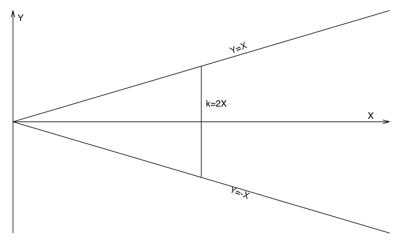
Figure 3: The whole of minisuperspace is conformally mapped into the wedge. The straight lines $X=\pm Y$ correspond to the two horizons, while the vertical line is the classical trajectory of a closed Universe.

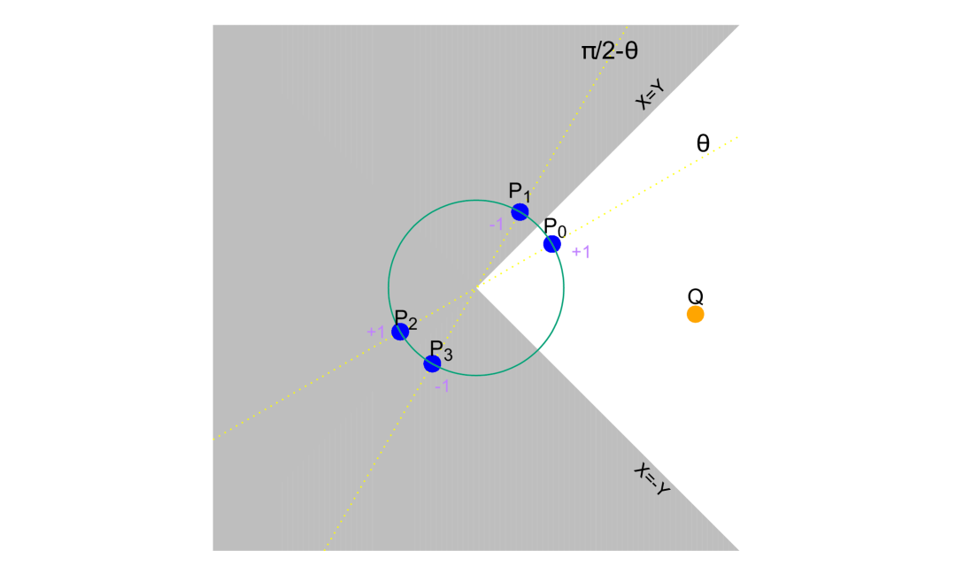
Figure 4: The Green’s function is a function of the point $Q$ and the source $P_{0}$. The positions and the charges of the images $P_{j}$’s are determined so as to satisfy the boundary conditions.

VI Treating the interaction as white noise

The methods developed in the previous sections are completely general and can be applied to any choice of the extra interaction terms using Eq. (53). In this section we will consider, as a particularly simple example, the case in which the additional interaction is given by white noise. Besides the mathematical simplicity there are also physical motivations for doing so. In fact, we can make the assumption that the additional terms that violate the Hamiltonian constraint can be used to model the effect of the underlying discreteness of spacetime on the evolution of the Universe.

Some approaches to Quantum Gravity (for instance GFT) suggest that an appropriate description of the gravitational interaction at a fundamental level is to be given in the language of third quantization Oriti:2013 . At this stage, one might make an analogy with the derivation of the Lamb shift in Quantum Electro-Dynamics (QED) and in effective stochastic approaches. As it is well known, the effect stems from the second quantized nature of the electromagnetic field. However, the same prediction can also be obtained if one holds the electromagnetic field as classical, but impose ad hoc conditions on the statistical distribution of its modes, which necessarily has to be the same as that corresponding to the vacuum state of QED. In this way, the instability of excited energy levels in atoms and the Lamb shift are seen as a result of the interaction of the electron with a stochastic background electromagnetic field Lamb-shift-SED ; Lamb-shift-spontaneous-emission-SED . However, in the present context we will not resort to a third quantization of the gravitational field, but instead put in ad hoc stochastic terms arising from interactions with degrees of freedom other than the scale factor. Certainly, our position here is weaker than that of Stochastic Electro-Dynamics (SED) (see Ref. de1983stochastic ; QM-SED and the works cited above), since a fundamental third quantized theory of gravity has not yet been developed to such an extent so as to make observable predictions in Cosmology. Therefore we are unable to give details about the statistical distribution of the gravitational degrees of freedom in what would correspond to the vacuum state. Our model should henceforth be considered as purely phenomenological and its link to the full theory will be clarified only when the construction of the latter will eventually be completed.

To be more specific, we treat the function $g$ in the perturbation as white noise. Stochastic noise is used to describe the interaction of a system with other degrees of freedom regarded as an environment. Hence we write

$$\langle g(\alpha,\phi)\rangle =0\leavevmode\nobreak\ ,$$ (62)

$$\langle g(\alpha,\phi)g(\alpha^{\prime},\phi^{\prime})\rangle =\delta(\alpha-\alpha^{\prime})\delta(\phi-\phi^{\prime})\leavevmode\nobreak\ ,$$ (63)

where $\langle\underline{\hskip 10.00002pt}\rangle$ denotes an ensemble average. It is straightforward to see that

$$\langle\psi^{(1)}\rangle=0\leavevmode\nobreak\ ,$$ (64)

which means that the ensemble average of the corrections to the wave function vanishes.

A more interesting quantity is represented by the second moment

$$\mathcal{F}(X_{1},Y_{1};X_{2},Y_{2})=\langle(\psi^{(1)}(X_{1},Y_{1}))^{*}\psi^{(1)}(X_{2},Y_{2})\rangle\leavevmode\nobreak\ .$$ (65)

In fact when evaluated at the same two points $\tilde{\mathcal{F}}(X,Y)\equiv\mathcal{F}(X,Y;X,Y)$, it represents the variance of the statistical fluctuations of the wave function at the point $(X,Y)$. Using Eqs. (15), (63) and (65) we get

$$\tilde{\mathcal{F}}(X,Y)=16\int_{X\geq|Y|}\mbox{d}X^{\prime}\,\mbox{d}Y^{\prime}\;(X^{\prime 2}-Y^{\prime 2})^{\frac{1}{2}}|\psi^{(0)}(X^{\prime},Y^{\prime})|^{2}\,|G(X-X^{\prime},Y-Y^{\prime})|^{2}\leavevmode\nobreak\ .$$ (66)

In order to obtain the correct expression of the integrand, one needs to use the transformation properties of the Dirac distribution, yielding

$$\langle g(\alpha,\phi)g(\alpha^{\prime},\phi^{\prime})\rangle=2(X^{2}-Y^{2})\delta(X-X^{\prime})\delta(Y-Y^{\prime})\leavevmode\nobreak\ .$$ (67)

Notice the resemblance of Eq. (65) with the two-point function evaluated to first order using Feynman rules for a scalar field in two dimensions interacting with a potential $(X^{2}-Y^{2})^{\frac{1}{2}}|\psi^{(0)}|^{2}$. Following this analogy, the variance $\tilde{\mathcal{F}}$ can be seen as a vacuum bubble.

Equation (66) implies that a white noise interaction is such that the different contributions to the modulus square of the perturbations add up incoherently.

VII Conserved charge and the choice of the inner product

Let us briefly discuss the rôle of the Noether charge and the choice of the inner product. Equation (18) is just a Klein-Gordon equation (with $\phi$ interpreted as time) with a potential $V(\alpha)=e^{4\alpha}-k^{2}$.

Equation (18) can be seen as the Euler-Lagrange equation of the Lagrangian

$$\mathcal{L}={\partial\psi^{*}\over\partial\alpha}{\partial\psi\over\partial\alpha}-{\partial\psi^{*}\over\partial\phi}{\partial\psi\over\partial\phi}+e^{4\alpha}\psi^{*}\psi\leavevmode\nobreak\ .$$ (68)

Since the Lagrangian is manifestly $U(1)$ invariant, the following conservation law holds as a consequence of Noether’s theorem

$$\partial_{\mu}j^{\mu}=0,$$ (69)

where

$$j_{\mu}=-i\left(\psi^{*}{\overset{\leftrightarrow}{\partial}\psi\over\partial\phi},\;\psi^{*}{\overset{\leftrightarrow}{\partial}\psi\over\partial\alpha}\right).$$ (70)

The corresponding Noether charge (obtained following the standard procedure) reads

$$Q=\int_{-\infty}^{\infty}\mbox{d}\alpha\;j_{\phi}\leavevmode\nobreak\ ,$$ (71)

and is conserved under time evolution

$${\mbox{d}Q\over\mbox{d}\phi}=0\leavevmode\nobreak\ .$$ (72)

Clearly, the conservation of $Q$ is in general incompatible with that of the $L^{2}$ norm of $\psi$, defined by

$$\lVert\psi\rVert_{L^{2}(\mathbb{R})}=\int_{-\infty}^{\infty}\mbox{d}\alpha\;|\psi|^{2}\leavevmode\nobreak\ .$$ (73)

Furthermore, the Noether charge $Q$ has no definite sign unless one considers only solutions with either positive or negative frequency, since a generic state admits a decomposition in terms of positive and negative frequency solutions of the free WDW equation. Such solutions span superselection sectors that are preserved by the Dirac observables identified in Ref. Ashtekar:2006D73 , and states in a given superselection sector satisfy a Schrödinger equation with a Hamiltonian $\pm\sqrt{\Theta}$. Within each sector, the conservation of the Hilbert norm holds true and Eq. (72) is an obvious consequence of energy conservation. As far as the free dynamics is concerned, it is perfectly legitimate to work in a superselection sector and use it to construct the (kinematical) Hilbert space (Ashtekar:2006, ; Ashtekar:2006D73, ). However, when the theory includes either non-linear interactions or potentials that depend on (internal) time, superselection no longer holds and both sectors have to be taken into account, thus naturally leading to a third quantization Isham:1992 . The non-equivalence of $Q$ and $\lVert\psi\rVert_{L^{2}(\mathbb{R})}$ can be easily seen for a wave packet (25), in which case one has

$$Q=\int_{-\infty}^{\infty}\mbox{d}k\;2k|A(k)|^{2}\leavevmode\nobreak\ .$$ (74)

Note that when $A(k)$ is supported only on one side of the real line, Eq. (72) can be interpreted as a conservation law for the average momentum. A similar interpretation is not available instead when both positive frequency and negative frequency solutions are present in the decomposition of the wave packet. For the reasons given above, a naive probabilistic interpretation of the theory along the lines of ordinary Quantum Mechanics does not seem possible in general. It is thus preferable to avoid using the designation of wave function for the classical field $\psi$.

The Noether charge of the semiclassical Universe considered in Section III can actually be computed analytically, and since it is conserved one can evaluate it in the simplest case, i.e. when the potential vanishes for $\alpha\to-\infty$. In fact when both $\alpha$ and $\phi$ are in a neighborhood of $-\infty$, i.e. close to the initial singularity, one can approximate the exact solution with a Gaussian wave packet (given by the WKB approximation, see Appendix A), which describes the evolution of the Universe in the expanding phase. We obtain

$$\psi\overset{{\alpha\to-\infty}}{{\approx}}c_{\overline{k}}\,b\sqrt{\frac{\pi}{2}}\exp\left\{\frac{i}{2}\left[\overline{k}\left(2\phi+\operatorname{arccosh}\left(\frac{\overline{k}}{e^{2\alpha}}\right)+\sqrt{1-\frac{e^{4\alpha}}{\overline{k}^{2}}}\right)-\frac{\pi}{2}\right]\right\}\exp\left[-\frac{b^{2}}{2}\left(\phi+\frac{1}{2}\operatorname{arccosh}\left({\overline{k}\over e^{2\alpha}}\right)\right)^{2}\right],$$ (75)

and then using Eq. (70) the charge density reads

$$j_{\phi}=|c_{\overline{k}}|^{2}\pi b^{2}\overline{k}\exp\left[-{b^{2}\over 4}\left(2\phi+\operatorname{arccosh}\left({\overline{k}\over e^{2\alpha}}\right)\right)^{2}\right]\leavevmode\nobreak\ .$$ (76)

For large negative values of $\alpha$ one can approximate the inverse hyperbolic function in the argument of the exponential as

$$\operatorname{arccosh}\left({\overline{k}\over e^{2\alpha}}\right)\overset{{\alpha\to-\infty}}{{\approx}}\log(2\overline{k})-2\alpha\leavevmode\nobreak\ ,$$ (77)

and hence reduce the evaluation of the charge to that of a Gaussian integral, leading to the result

$$Q=|c_{\overline{k}}|^{2}b\,\pi^{3/2}\;\overline{k}\leavevmode\nobreak\ .$$ (78)

From the above analysis we conclude that the quantum conservation law leads, in the classical limit, to momentum conservation. We recall that classically the momentum is related to the derivative of the scalar field w.r.t. proper time, as

$$\overline{k}=a^{3}\dot{\phi}\leavevmode\nobreak\ .$$ (79)

VIII Conclusions

Motivated by LQC and GFT we considered an extension of WDW minisuperspace cosmology with additional interaction terms representing a self-interaction of the Universe. Such terms can be seen as a particular case of the model considered in Ref. Calcagni:2012 , which was proposed as an approach to quantum dynamics of inhomogeneous cosmology. In general, inhomogeneities would lead to non-linear differential equations for the quantum field. This is indeed the case when the “wave function” of the Universe is interpreted as a quantum field or even as a classical field describing the hydrodynamics limit of GFT.

In the framework of a first quantized cosmology, we only considered linear modifications of the theory in order to secure the validity of the superposition principle. Our work represents a first step towards a more general study, that should take into account non-linear and possibly non-local interactions in minisuperspace. However, the way such terms arise, their exact form, and even the precise way in which minisuperspace dynamics is derived from fundamental theories of Quantum Gravity should be dictated from the full theory itself.

Assuming that the additional interactions are such that deviations from the Friedmann equation are small, we developed general perturbative methods which allowed us to solve the modified WDW equation. We considered a closed FLRW Universe filled with a massive scalar field to define an internal time, for which wave packets solutions are known explicitly and propagate with no dispersion. A modified WDW equation is then obtained in the large volume limit of a particular GFT inspired extension of LQC for a closed FLRW Universe. Perturbative methods are then used to find the corrections given by self-interactions of the Universe to the exact solution given in Ref. Kiefer:1988 . To this end, the Feynman propagator of the WDW equation is evaluated exactly by means of a conformal map in minisuperspace and (after a Wick rotation) using the method of the image charges that is familiar from electrostatics. This is potentially interesting as a basic building block for any future perturbative analysis of non-linear minisuperspace dynamics for a closed Universe.

A Helmoltz-like equation was obtained from WDW when the extra interaction does not depend on the internal time. Its Green’s kernel was evaluated exactly and turned out to depend on a free parameter $\eta$ related to the choice of boundary conditions. Further research must be carried over to link $\eta$ to different boundary proposals.

We illustrated our perturbative approach in the simple and physically motivated case in which the perturbation is presented by white noise. In this phenomenological model the stochastic interaction term can be seen as describing the interaction of the cosmological background with other degrees of freedom of the gravitational field. Calculating the variance of the statistical fluctuations of the wave function, we found that a white noise interaction is such that the different contributions to the modulus square of the perturbations add up incoherently.

Appendix A WKB approximation of the elementary solutions and asymptotics of the wave packets

Since Eq. (22) has the form of a time-independent Schr̈odinger equation, it is possible to construct approximate solutions using the WKB method.

For a given $k$, we divide the real line in three regions, with a neighborhood of the classical turning point in the middle. The classical turning point is defined as the point where the potential is equal to the energy

$$\alpha_{k}=\frac{1}{2}\log{k}\leavevmode\nobreak\ .$$ (80)

The WKB solution to first order in the classically allowed region $]-\infty,\alpha_{k}-\epsilon]$ (with $\epsilon$ an appropriately chosen real number, see below) is

$$C_{k}^{I}=\frac{2}{(k^{2}-e^{4\alpha})^{1/4}}\cos\left(\frac{1}{2}\sqrt{k^{2}-e^{4\alpha}}-\frac{k}{2}\mbox{arccoth}\left(\frac{k}{\sqrt{k^{2}-e^{4\alpha}}}\right)+\frac{\pi}{4}\right)\leavevmode\nobreak\ ,$$ (81)

and reduces to a plane wave in the allowed region for $\alpha\ll\alpha_{k}$. The presence of the barrier fixes the amplitude and the phase relation of the incoming and the reflected wave through the matching conditions.

The solution in the classically forbidden region $[\alpha_{k}+\epsilon,+\infty[$ is instead exponentially decreasing as it penetrates the potential barrier and reads

$$C_{k}^{III}=\frac{1}{(e^{4\alpha}-k^{2})^{1/4}}\exp\left(-\frac{1}{2}\sqrt{e^{4\alpha}-k^{2}}+\frac{k}{2}\arctan\left(\frac{k}{\sqrt{e^{4\alpha}-k^{2}}}\right)\right)\leavevmode\nobreak\ .$$ (82)

Finally, in the intermediate region $]\alpha_{k}-\epsilon,\alpha_{k}+\epsilon[$ any semiclassical method would break down, hence the Schrödinger equation must be solved exactly using the linearized potential

$$V(\alpha)\simeq V(\alpha_{k})+V^{\prime}(\alpha_{k})(\alpha-\alpha_{k})=4e^{4\alpha_{k}}(\alpha-\alpha_{k})=4k^{2}(\alpha-\alpha_{k})\leavevmode\nobreak\ .$$ (83)

In this intermediate regime, Eq. (22) can be rewritten as the well-known Airy equation

$$\frac{\mbox{d}^{2}C_{k}^{II}}{\mbox{d}t^{2}}-tC_{k}^{II}=0\leavevmode\nobreak\ ,$$ (84)

where the variable $t$ is defined as

$$t=(4k^{2})^{1\over 3}(\alpha-\alpha_{k})\leavevmode\nobreak\ .$$ (85)

Of the two independent solutions of Eq. (84), only the Airy function $\mbox{Ai}(t)$ satisfies the boundary condition, and hence we conclude that

$$C_{k}^{II}=c\;Ai(t)\leavevmode\nobreak\ ,$$ (86)

where $c$ is a constant that has to be determined by matching the asymptotics of $\mbox{Ai}(t)$ with the WKB approximations on both sides of the turning point. Hence we get that, for $t\ll 0$

$$\mbox{Ai}(t)\approx\frac{\cos\left(\frac{2}{3}|t|^{3/2}-\frac{\pi}{4}\right)}{\sqrt{\pi}|t|^{1/4}}\leavevmode\nobreak\ ,$$ (87)

while for $t\gg 0$

$$\mbox{Ai}(t)\approx\frac{e^{-\frac{2}{3}t^{3/2}}}{2\sqrt{\pi}t^{1/4}}\leavevmode\nobreak\ .$$ (88)

We thus fix $c=2\sqrt{\pi}$. Note that the arbitrariness in the choice of $\epsilon$ can be solved, e.g. by requiring the point $\alpha_{k}-\epsilon$ to coincide with the first zero of the Airy function.

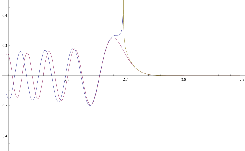
Figure 5: The blue and the yellow curve represent, the WKB approximation of the wave function in the classically allowed and in the forbidden region, respectively. They both diverge at the classical turning point. The Airy function is represented in red. The value $k=220$ was chosen.

The WKB approximation improves at large values of $k$, as one should expect from a method that is semiclassical in spirit. Yet it allows one to capture some effects that are genuinely quantum, such as the barrier penetration and the tunneling effect.

From the approximate solution we have just found, we can construct wave packets as in Ref. Kiefer:1988 . We thence restrict our attention to the classically allowed region and the corresponding approximate solutions, i.e. $C_{k}^{I}(\alpha)$ for $\alpha\ll\alpha_{k}=\frac{1}{2}\log{k}$ and compute the integral in Eq. (25). If the Gaussian representing the amplitudes of the monochromatic modes is narrow peaked, i.e. its variance $b^{2}$ is small enough, we can approximate the amplitude in Eq. (81) with that corresponding to the mode with the mean frequency $\overline{k}$. Thus, introducing the constant

$$c_{\overline{k}}=\frac{2}{(\overline{k}^{2}-e^{4\alpha})^{1/4}}\frac{1}{\pi^{1/4}\sqrt{b}}\leavevmode\nobreak\ ,$$ (89)

we have

$$\psi(\alpha,\phi)\simeq c_{\overline{k}}\int_{-\infty}^{\infty}\mbox{d}k\;e^{-\frac{(k-\overline{k})^{2}}{2b^{2}}}\cos\left(\frac{1}{2}\sqrt{k^{2}-e^{4\alpha}}-\frac{k}{2}\mbox{arccoth}\left(\frac{k}{\sqrt{k^{2}-e^{4\alpha}}}\right)+\frac{\pi}{4}\right)e^{ik\phi}\leavevmode\nobreak\ .$$ (90)

Moreover,

$$k\,\mbox{arccoth}\left(\frac{k}{\sqrt{k^{2}-e^{4\alpha}}}\right)=k\operatorname{arccosh}\frac{k}{e^{2\alpha}}\simeq k\operatorname{arccosh}\frac{\overline{k}}{e^{2\alpha}}\leavevmode\nobreak\ .$$ (91)

The last approximation in the equation above holds as the derivative of the inverse hyperbolic function turns out to be much smaller than unity in the allowed region. Furthermore, the term approximated in Eq. (91) dominates over the square root in the argument of the cosine in the integrand in the r.h.s. of Eq. (90), so we can consider the latter as a constant. Hence, we can write

$$\psi(\alpha,\phi)\simeq c_{\overline{k}}\int_{-\infty}^{\infty}\mbox{d}k\;e^{-\frac{(k-\overline{k})^{2}}{2b^{2}}}\cos\left(\Lambda k+\delta\right)e^{ik\phi}\leavevmode\nobreak\ ,$$ (92)

where we have introduced the notation

$$\Lambda \equiv\frac{1}{2}\operatorname{arccosh}\frac{\overline{k}}{e^{2\alpha}}\leavevmode\nobreak\ ,$$ (93)

$$\delta \equiv\frac{1}{2}\sqrt{\overline{k}^{2}-e^{4\alpha}}-\frac{\pi}{4}\leavevmode\nobreak\ .$$ (94)

for convenience. Using Euler’s formula we can express the cosine in the integrand in the r.h.s. of Eq. (92) in terms of complex exponentials and evaluate $\psi(\alpha,\phi)$. In fact, defining

$$P_{\overline{k}}\equiv e^{i\left(\overline{k}(\Lambda+\phi)+\delta\right)}\leavevmode\nobreak\ ,\leavevmode\nobreak\ \hskip 10.00002ptQ_{\overline{k}}\equiv e^{-i\left(\overline{k}(\Lambda-\phi)+\delta\right)}\leavevmode\nobreak\ ,$$ (95)

we have

$$\psi(\alpha,\phi)\simeq\frac{c_{\overline{k}}}{2}\int_{-\infty}^{\infty}\mbox{d}k\;e^{-\frac{(k-\overline{k})^{2}}{2b^{2}}}\left(e^{i(k-\overline{k})(\Lambda+\phi)}P_{\overline{k}}+e^{-i(k-\overline{k})(\Lambda-\phi)}Q_{\overline{k}}\right)\leavevmode\nobreak\ .$$ (96)

Shifting variables and performing the Gaussian integrations we get the result as in Ref. Kiefer:1988

$$\psi(\alpha,\phi)\simeq c_{\overline{k}}\sqrt{\frac{\pi}{2}}b\left(e^{-\frac{b^{2}}{2}(\Lambda+\phi)^{2}}P_{\overline{k}}+e^{-\frac{b^{2}}{2}(\Lambda-\phi)^{2}}Q_{\overline{k}}\right)\leavevmode\nobreak\ .$$ (97)

Appendix B Orthogonality of the MacDonald functions

It was proved in Refs. Szmytkowski ; Yakubovich ; Passian that

$$\int_{0}^{\infty}\frac{\mbox{d}x}{x}\;K_{i\nu}(kx)K_{i\nu^{\prime}}(kx)=\frac{\pi^{2}\delta(\nu-\nu^{\prime})}{2\nu\sinh(\pi\nu)}\leavevmode\nobreak\ ,$$ (98)

which expresses the orthogonality of the MacDonald functions of imaginary order. Performing a change of variables, the above formula can be recast in the form

$$\int_{-\infty}^{\infty}\mbox{d}\alpha\;K_{i\frac{h}{2}}\left(\frac{e^{2\alpha}}{2}\right)K_{i\frac{h^{\prime}}{2}}\left(\frac{e^{2\alpha}}{2}\right)=\frac{\pi^{2}\delta(h-h^{\prime})}{h\sinh(\pi\frac{h}{2})}\leavevmode\nobreak\ ,$$ (99)

which is convenient for the applications considered in this work. For large values of $k$ it is equivalent to the normalization used in Section II

$$\int_{-\infty}^{\infty}\mbox{d}\alpha\;\psi^{*}_{k^{\prime}}(\alpha,\phi)\psi_{k}(\alpha,\phi)=\frac{\pi^{2}}{2}\delta(k-k^{\prime})\leavevmode\nobreak\ .$$ (100)

References

- (1) C. Rovelli, Class.Quant.Grav. 32, 124005 (2015), 1506.00927.
- (2) J. Halliwell, Time in quantum cosmology, in Conceptual problems of quantum gravity. Proceedings, Osgood Hill Conference, edited by Ashtekar, A. and Stachel, J., pp. 204–210, Birkhäuser, 1988.
- (3) D. A. Craig and P. Singh, AIP Conf. Proc. 1232, 275 (2010).
- (4) S. B. Giddings and A. Strominger, Nucl. Phys. B321, 481 (1989).
- (5) D. Oriti, Group Field Theory and Loop Quantum Gravity, 2014, 1408.7112.
- (6) G. Calcagni, S. Gielen, and D. Oriti, Class.Quant.Grav. 29, 105005 (2012), 1201.4151.
- (7) A. Ashtekar, M. Bojowald, and J. Lewandowski, Adv. Theor. Math. Phys. 7, 233 (2003), gr-qc/0304074.
- (8) D. Oriti and L. Sindoni, New J. Phys. 13, 025006 (2011), 1010.5149.
- (9) A. Ashtekar, T. Pawlowski, P. Singh, and K. Vandersloot, Phys.Rev. D75, 024035 (2007), gr-qc/0612104.
- (10) C. Kiefer, Phys.Rev. D38, 1761 (1988).
- (11) A. M. Cetto and L. de la Pea, Phys. Rev. A 37, 1952 (1988).
- (12) L. De La Pena, Stochastic Processes Applied to Physics and other Related Fields , 428 (1983).
- (13) A. M. Cetto and L. de la Peña, Physica Scripta 1988, 27 (1988).
- (14) L. de la Peña‐Auerbach and A. M. Cetto, Journal of Mathematical Physics 18, 1612 (1977).
- (15) A. Ashtekar, A. Corichi, and P. Singh, Phys. Rev. D77, 024046 (2008), 0710.3565.
- (16) A. Corichi, T. Vukasinac, and J. A. Zapata, AIP Conf. Proc. 977, 64 (2008), 0711.0788.
- (17) A. Ashtekar, T. Pawlowski, and P. Singh, Phys. Rev. D74, 084003 (2006), gr-qc/0607039.
- (18) C. J. Isham, Canonical quantum gravity and the problem of time, in 19th International Colloquium on Group Theoretical Methods in Physics (GROUP 19) Salamanca, Spain, June 29-July 5, 1992, 1992, gr-qc/9210011.
- (19) S. W. Hawking, Pontif. Acad. Sci. Scr. Varia 48, 563 (1982).
- (20) J. B. Hartle and S. W. Hawking, Phys. Rev. D28, 2960 (1983).
- (21) A. Vilenkin, Phys. Rev. D37, 888 (1988).
- (22) H.-H. Zhang, K.-X. Feng, S.-W. Qiu, A. Zhao, and X.-S. Li, Chin. Phys. C34, 1576 (2010), 0811.1261.
- (23) A. Di Sessa, Phys. Rev. D9, 2926 (1974).
- (24) M. Bojowald and F. Hinterleitner, Phys. Rev. D66, 104003 (2002), gr-qc/0207038.
- (25) M. Bojowald and K. Vandersloot, Loop quantum cosmology and boundary proposals, in On recent developments in theoretical and experimental general relativity, gravitation, and relativistic field theories. Proceedings, 10th Marcel Grossmann Meeting, MG10, Rio de Janeiro, Brazil, July 20-26, 2003. Pt. A-C, pp. 1089–1103, 2003, gr-qc/0312103.
- (26) D. Oriti, (2013), 1310.7786.
- (27) K. Yasue, Journal of Statistical Physics 16, 113 (1977).
- (28) M. Bojowald, P. A. Hoehn, and A. Tsobanjan, Class. Quant. Grav. 28, 035006 (2011), 1009.5953.
- (29) A. Ashtekar, T. Pawlowski, and P. Singh, Phys. Rev. D73, 124038 (2006), gr-qc/0604013.
- (30) G. Calcagni, S. Gielen, and D. Oriti, Class. Quant. Grav. 28, 125014 (2011), 1011.4290.
- (31) R. Szmytkowski and S. Bielski, Journal of Mathematical Analysis and Applications 365, 195 (2010).
- (32) S. Yakubovich, Opuscula Mathematica 26, 161 (2006).
- (33) A. Passian, H. Simpson, S. Kouchekian, and S. Yakubovich, Journal of Mathematical Analysis and Applications 360, 380 (2009).