Spin torque and Nernst effects in Dzyaloshinskii-Moriya ferromagnets

Abstract

We predict that a temperature gradient can induce a magnon-mediated intrinsic torque in systems with non-trivial magnon Berry curvature. With the help of a microscopic linear response theory of nonequilibrium magnon-mediated torques and spin currents we identify the interband and intraband components that manifest in ferromagnets with Dzyaloshinskii–Moriya interactions and magnetic textures. To illustrate and assess the importance of such effects, we apply the linear response theory to the magnon-mediated spin Nernst and torque responses in a kagome lattice ferromagnet.

Studies of the spin degree of freedom in spintronics Žutić et al. (2004) naturally extend to include the interplay between the energy and spin flows in the field of spincaloritronics Bauer et al. (2012); Goennenwein and Bauer (2012). Improved efficiency in interconversion between energy and spin Weiler et al. (2013) could result in important applications, e.g., for energy harvesing, cooling, and magnetization control Hatami et al. (2007); Bauer et al. (2010); Kovalev and Tserkovnyak (2009); Cahaya et al. (2014); Kovalev and Tserkovnyak (2010); Kovalev and Güngördü (2015). Magnetic insulators such as yttrium iron garnet (YIG) or Lu₂V₂O₇ offer a perfect playground for spincaloritronics where due to the absence of electron continuum the dissipation can be lowered as only the spin and energy matter Kajiwara et al. (2010); Onose et al. (2010); Uchida et al. (2010). It has already been demonstrated in recent experiments that energy currents can be used for magnetization control Torrejon et al. (2012); Jiang et al. (2013). This opens new possibilities for applications of magnon-mediated torques in racetrack memories Parkin et al. (2008); Brataas et al. (2012), and even in quantum information manipulations Kim et al. (2015).

As we show in this study, the magnon-mediated torque is closely related to the magnon-mediated thermal Hall effect. The latter has been observed in Lu₂V₂O₇ Onose et al. (2010) and explained by the Berry curvature of magnon bands Matsumoto and Murakami (2011); Matsumoto et al. (2014); Katsura et al. (2010) where the physics is reminiscent of the anomalous Hall effect Sundaram and Niu (1999). The possibility of the magnon edge currents and tunable topology of the magnon bands has also been discussed in the context of magnetic insulators Matsumoto and Murakami (2011); Zhang et al. (2013); Mook et al. (2014, 2014). In a recent experiment, the magnon-mediated thermal Hall effect showed the sign reversal with changes in temperature or magnetic field in the kagome magnet Cu(1-3, bdc) Hirschberger et al. (2015). Since magnons also carry spin it would be natural to also study how spin currents can be generated from temperature gradients, i.e., the spin Nernst effect, in materials with nontrivial topology of magnon bands. However, both the magnon-mediated torque and the spin Nernst effect have not been addressed in systems with non-trivial magnon Berry curvature. Such calculations inevitably require generalizations of linear response methods developed in sixties and seventies Luttinger (1964); Smrcka and Streda (1977) to bosonic systems and consideration of the spin current analog of the energy magnetization contribution Qin et al. (2011).

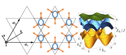
Figure 1: (Color online) Left: Two-dimensional kagome lattice with lattice vectors $\boldsymbol{a}_{1}$ and $\boldsymbol{a}_{2}$ where atoms are placed in the corners of triangles. DMI are shown by vectors perpendicular to the bonds. The DMI of strength $D_{1}$ point into the page while the Rashba-like DMI of strength $D_{2}$ lie in the page. Right: The three magnon bands are plotted for the case of broken mirror symmetry with respect to the kagome plane due to the Rashba-like DMI. The direction of the spin density is given by $\mathbf{m}=\hat{x}\sin(\pi/6)+\hat{z}\cos(\pi/6)$.

In this Rapid Communication, we predict that a temperature gradient can induce a magnon-mediated intrinsic torque in systems with non-trivial magnon Berry curvature. To this end, we formulate a microscopic linear response theory to temperature gradients for ferromagnets with multiple magnon bands. We follow the Luttinger approach of the gravitational scalar potential Luttinger (1964); Tatara (2015). Our theory is capable of capturing the nontrivial topology of magnon bands resulting from the Dzyaloshinskii–Moriya interactions (DMI) Moriya (1960); Dzyaloshinsky (1958). An additional vector potential corresponding to the magnetic texture can be readily introduced in our approach via minimal coupling. We note that the predicted magnon-mediated torques are bosonic analogs of the spin-orbit torques Bernevig and Vafek (2005); Manchon and Zhang (2008); Matos-Abiague and Rodríguez-Suárez (2009); Chernyshov et al. (2009); Garate and MacDonald (2009); Endo et al. (2010); Fang et al. (2011); Liu et al. (2012); Kurebayashi et al. (2014); Garello et al. (2013). We find that torques due to Dzyaloshinskii–Moriya interactions (DM torques) can only arise in systems lacking the center of inversion. This is in contrast to the the magnon-mediated spin Nernst effect. Finally, we express the intrinsic contribution to the DM torque via the mixed Berry curvature calculated with respect to the variation of the magnetization and momentum Sundaram and Niu (1999). We apply our linear response theory to the magnon-mediated spin Nernst and torque responses in a kagome lattice ferromagnet. We note that the latter can be detected by studying the magnetization dynamics while the former can be detected by the inverse spin Hall effect.

Microscopic theory.— We consider a noninteracting boson Hamiltonian describing the magnon fields:

$$\mathcal{H}=\int d\mathbf{r}\Psi^{\dagger}(\mathbf{r})H\Psi(\mathbf{r}),$$ (1)

where $H$ is a Hermitian matrix of the size $N\times N$ and $\Psi^{\dagger}(\mathbf{r})=[a_{1}^{\dagger}(\mathbf{r}),\ldots,a_{N}^{\dagger}(\mathbf{r})]$) describes $N$ bosonic fields corresponding to the number of modes within a unit cell (or the number of spin-wave bands). Hamiltonian in Eq. (1) can also account for smooth magnetic textures via minimal coupling to the texture-induced vector potential $\boldsymbol{\cal{A}}$ via additional term $(\boldsymbol{\cal{A}}_{\alpha}\cdot\mathbf{m})j^{s}_{\alpha}$ where $j^{s}_{\alpha}$ is the magnon spin current Kovalev and Tserkovnyak (2012); Tatara (2015). The Fourier transformed Hamiltonian is:

$$\mathcal{H}=\sum_{\mathbf{k}}a_{k}^{\dagger}H(\mathbf{k})a_{k},$$ (2)

where $a_{k}^{\dagger}$ is the Fourier transformed vector of creation operators. Hamiltonian in Eq. (2) can be diagonalized by a unitary matrix $T_{k}$, i.e. $\mathcal{E}_{k}=T_{k}^{\dagger}H(\mathbf{k})T_{k}$ and $T_{k}^{\dagger}T_{k}=1_{N\times N}$ where $\mathcal{E}_{k}$ is the diagonal matrix of band energies, and $1_{N\times N}$ is the $N\times N$ unit matrix. As it was shown by Luttinger Luttinger (1964), the effect of the temperature gradient can be replicated by introducing a perturbation to Hamiltonian in Eq. (1):

$$\mathcal{H}^{{}^{\prime}}=\dfrac{1}{2}\int d\mathbf{r}\Psi^{\dagger}(\mathbf{r})\left(H\chi+\chi H\right)\Psi(\mathbf{r}),$$ (3)

where the nonequilibrium magnon-mediated field can be treated as a linear response to the perturbation in Eq. (3) and $\partial_{i}\chi=\partial_{i}T/T$.

The nonequilibrium magnon-mediated field can be calculated by invoking arguments similar to those for the spin-orbit torque Garate and MacDonald (2009); Géranton et al. (2015); Qaiumzadeh et al. (2015):

$$\mathbf{h}_{\text{tot}}=\mathbf{h}+\mathbf{h}^{{}^{\prime}}=-\bigl{\langle}\partial_{\mathbf{m}}\mathcal{H}\bigr{\rangle}_{ne}-\bigl{\langle}\partial_{\mathbf{m}}\mathcal{H}^{{}^{\prime}}\bigr{\rangle}_{eq},$$ (4)

where the averaging is done either over the equilibrium or nonequilibrium state induced by the temperature gradient, and $\mathbf{m}$ is a unit vector in the direction of the spin density $s$. The magnon-mediated torque can be expressed as $\boldsymbol{\mathcal{T}}=\mathbf{m}\times\mathbf{h}_{\text{tot}}$ leading to modification of the Landau-Lifshitz-Gilbert equation, i.e., $s(1+\alpha\mathbf{m}\times)\dot{\mathbf{m}}=\mathbf{m}\times\mathbf{H}_{\text{eff}}+\boldsymbol{\mathcal{T}}$ where $\mathbf{H}_{\text{eff}}$ is the effective magnetic field. We are also concerned with the magnon current carrying spin which has two components:

$$\mathbf{J}_{\text{tot}}=\bigl{\langle}\mathbf{J}\bigr{\rangle}_{ne}+\bigl{\langle}\mathbf{J}^{{}^{\prime}}\bigr{\rangle}_{eq},$$ (5)

where the first component, $\mathbf{J}=\int d\mathbf{r}\Psi^{\dagger}(\mathbf{r})\mathbf{v}\Psi(\mathbf{r})$, does not depend on the temperature gradient and the second component, $\mathbf{J}^{{}^{\prime}}=(1/2)\int d\mathbf{r}\Psi^{\dagger}(\mathbf{r})\left(\mathbf{v}\chi+\chi\mathbf{v}\right)\Psi(\mathbf{r})$, is proportional to the temperature gradient. The latter contribution is related to the spin current analog of the energy magnetization Qin et al. (2011). Here the velocity operator is given by $\mathbf{v}=(1/i\hbar)[\mathbf{r},H]$. The magnon current density $\mathbf{j}$ is introduced in a standard way from the continuity equation $\dot{\rho}+\boldsymbol{\nabla}\cdot\mathbf{j}(\mathbf{r})=0$ where $\rho$ is the density of magnons. In our discussion, we employ the expression for the energy current density, $\mathbf{j}^{Q}(\mathbf{r})=(1/2)\Psi^{\dagger}(\mathbf{r})(\mathbf{v}H+H\mathbf{v})\Psi(\mathbf{r})$, and the macroscopic energy current $\mathbf{J}^{Q}=\int d\mathbf{r}\mathbf{j}^{Q}(\mathbf{r})$ corresponding to the continuity equation $\dot{\rho}_{E}+\boldsymbol{\nabla}\cdot\mathbf{j}^{Q}(\mathbf{r})=0$ with $\rho_{E}$ being the energy density. Note that we omitted the component of $\mathbf{j}^{Q}$ proportional to $\partial_{i}\chi$ as it is irrelevant to our discussion. Within the linear response theory, the response of an operator X to temperature gradient becomes:

$$\bigl{\langle}X_{i}\bigr{\rangle}_{ne}=\lim_{\Omega\rightarrow 0}\left\{[\Pi_{ij}^{R}(\Omega)-\Pi_{ij}^{R}(0)]/i\Omega\right\}\partial_{j}\chi,$$ (6)

where $\mathbf{X}$ is either spin current $-\hbar\mathbf{J}$ or nonequilibrium field $\mathbf{h}=-\partial_{\mathbf{m}}H$, $\Pi_{ij}^{R}(\Omega)=\Pi_{ij}(\Omega+i0)$ is the retarded correlation function related to the following correlator in Matsubara formalism, $\Pi_{ij}(i\Omega)=-\int_{0}^{\beta}d\tau e^{i\Omega\tau}\bigl{\langle}T_{\tau}X_{i}J_{j}^{Q}\bigr{\rangle}$. Note that the energy current originates from the expression $\mathcal{\dot{H}}^{{}^{\prime}}=(i/\hbar)[\mathcal{H},\mathcal{H}^{{}^{\prime}}]=\mathbf{J}^{Q}\boldsymbol{\partial}\chi$.

We calculate the correlator in Eq. (6) by considering the simplest bubble diagram for $\Pi_{ij}$ and performing the analytic continuation. We express the result through a response tensor $t_{ij}=t_{ij}^{\text{I}}+t_{ij}^{\text{II}}$ such that $X_{i}=-t_{ij}\partial_{j}\chi$ Not :

$$\begin{array}[]{c}t_{ij}^{\text{I}}=\dfrac{1}{\hbar}{\displaystyle\int}\dfrac{d\omega}{2\pi}g(\omega)\dfrac{d}{d\omega}\mbox{Re}\mbox{Tr}\bigl{\langle}X_{i}G^{R}\mathcal{J}_{j}G^{A}-X_{i}G^{R}\mathcal{J}_{j}G^{R}\bigr{\rangle},\\ t_{ij}^{\text{II}}=\dfrac{1}{\hbar}{\displaystyle\int}\dfrac{d\omega}{2\pi}g(\omega)\mbox{Re}\mbox{Tr}\bigl{\langle}X_{i}G^{R}\mathcal{J}_{j}\dfrac{dG^{R}}{d\omega}-X_{i}\dfrac{dG^{R}}{d\omega}\mathcal{J}_{j}G^{R}\bigr{\rangle},\end{array}$$ (7)

where $g(\omega)$ is the Bose distribution function $g(\omega)=1/[\exp(\hbar\omega/k_{B}T)-1]$, $G^{R}=\hbar(\hbar\omega-H+i\Gamma)^{-1}$, $G^{A}=\hbar(\hbar\omega-H-i\Gamma)^{-1}$, and $\boldsymbol{\mathcal{J}}=(\mathbf{v}H+H\mathbf{v})/2$. For practical purposes, we Fourier transform Eq. (7) which leads to additional momentum integration and momentum transformed terms, i.e. $G^{R}(\mathbf{k})=\hbar(\hbar\omega-H(\mathbf{k})+i\Gamma)^{-1}$, $\mathbf{h}_{k}=-\partial_{\mathbf{m}}H(\mathbf{k})$, $\mathbf{v}_{k}=\partial_{\hbar\mathbf{k}}H(\mathbf{k})$, and $\boldsymbol{\mathcal{J}}{}_{k}=(\mathbf{v}_{k}H(\mathbf{k})+H(\mathbf{k})\mathbf{v}_{k})/2$. The approximation we are using can be improved by performing the disorder averaging which is indicated by brackets in Eq. (7) . In addition, interactions with phonons can be also taken into account and can result in additional dissipative corrections to the torque. Throughout this paper, we adopt a simple phenomenological treatment by relating the quasiparticle broadening to the Gilbert damping, i.e. $\Gamma=\alpha\hbar\omega$.

Berry curvature formulation.— It is very insightful to carry out the frequency integrations in Eq. (7), keeping only the two leading orders in $\Gamma$ and combining the linear response result with the nonequilibrium contribution $\mathbf{h}^{{}^{\prime}}$ in Eq. (4) or $\mathbf{J}^{{}^{\prime}}$ in Eq. (5). To carry the integrations in Eq. (7) we use the diagonal basis defined by rotation matrices $T_{k}$, and transform the contributions $\mathbf{h}^{{}^{\prime}}$ and $\mathbf{J}^{{}^{\prime}}$ to an integral over energies following the approach of Smrcka and Streda Smrcka and Streda (1977); Matsumoto et al. (2014). Using the covariant derivative we calculate the rotated velocity, $T_{k}^{\dagger}\hbar\mathbf{v}_{k}T_{k}=\partial_{\mathbf{k}}\mathcal{E}_{k}-i\boldsymbol{\mathcal{A}}_{k}\mathcal{E}_{k}+i\mathcal{E}_{k}\boldsymbol{\mathcal{A}}_{k}$, and nonequilibrium field, $T_{k}^{\dagger}\mathbf{h}_{k}T_{k}=\partial_{\mathbf{m}}\mathcal{E}_{k}-i\boldsymbol{\mathcal{A}}_{m}\mathcal{E}_{k}+i\mathcal{E}_{k}\boldsymbol{\mathcal{A}}_{m}$, where $\boldsymbol{\mathcal{A}}_{k}=iT_{k}^{\dagger}\partial_{\mathbf{k}}T_{k}$ and $\boldsymbol{\mathcal{A}}_{m}=iT_{k}^{\dagger}\partial_{\mathbf{m}}T_{k}$. Substituting these in Eq. (7) we identify the intraband and interband contributions to the response tensor Not :

$$\begin{array}[]{c}t_{ij}^{\text{intra}}=\dfrac{1}{V}{\displaystyle\sum_{\mathbf{k}}{\displaystyle\sum_{n=1}^{N}}\dfrac{1}{2\Gamma_{k}}(\partial_{x_{i}}\varepsilon_{nk})(\partial_{k_{j}}\varepsilon_{nk})\varepsilon_{nk}g^{\prime}(\varepsilon_{nk})},\\ t_{ij}^{\text{inter}}=\dfrac{k_{B}T}{V}{\displaystyle\sum_{\mathbf{k}}}{\displaystyle\sum_{n=1}^{N}}c_{1}[g(\varepsilon_{nk})]\Omega_{x_{i}k_{j}}^{n}(\mathbf{k}),\end{array}$$ (8)

where $x_{i}$ is either $m_{i}$ or $k_{i}$, $\varepsilon_{nk}=[\mathcal{E}_{k}]_{nn}$, $\Gamma_{nk}=\alpha\varepsilon_{nk}$, $g^{\prime}(\varepsilon_{nk})=(2k_{B}T)^{-1}\{1-\cosh(\varepsilon_{nk}/k_{B}T)\}^{-1}$, $c_{1}[x]=\int_{0}^{x}dt\ln[(1+t)/t]=(1+x)\ln[1+x]-x\ln x$, $V$ is volume, and we introduced the Berry curvature of $n$-th band:

$$\Omega_{x_{i}k_{j}}^{n}(\mathbf{k})=i[(\partial_{x_{i}}T_{k}^{\dagger})(\partial_{k_{j}}T_{k})-(\partial_{k_{j}}T_{k}^{\dagger})(\partial_{x_{i}}T_{k})]_{nn}.$$ (9)

Such Berry curvatures naturally appear in discussions of semiclassical equations of motion for Hamiltonians with slowly varying parameters Sundaram and Niu (1999). Derivation of Eq. (8) (see supplemental material Not ) should also hold for fermion systems given that $c_{1}(\varepsilon_{nk})=-\int_{\varepsilon_{nk}}^{\infty}\eta\frac{dn_{F}(\eta)}{d\eta}d\eta$ where the Fermi-Dirac distribution $n_{F}$ replaces $g$ Freimuth et al. (2016). By applying the time reversal transformation, i.e. $\mathbf{k}\rightarrow-\mathbf{k}$, $\mathbf{m}\rightarrow-\mathbf{m}$, $\Omega_{x_{i}k_{j}}^{n}\rightarrow-\Omega_{-x_{i}-k_{j}}^{n}$, to Eqs. (8) we recover the transformation properties of $t_{ij}^{\text{intra}}$ and $t_{ij}^{\text{inter}}$ under the magnetization reversal. In particular, it is clear that $t_{ij}^{\text{intra}}$ is even under the magnetization reversal and is divergent as $\Gamma\rightarrow 0$. On the other hand, $t_{ij}^{\text{inter}}$ is odd under the magnetization reversal and corresponds to the intrinsic contribution independent of $\Gamma$. In terms of spin torques, the former corresponds to the field-like torque and the latter to the anti-damping (or dissipative) intrinsic torque.

Model.— We apply our theory to the magnon current and torque response of a kagome lattice ferromagnet with DMI (see Fig. 1). The exchange and DMI terms in the Hamiltonian are given by Moriya (1960); Dzyaloshinsky (1958):

$${\cal H}=-\frac{1}{2}J\sum_{i\neq j}\mathbf{S}_{i}\cdot\mathbf{S}_{j}+\frac{1}{2}\sum_{i\neq j}\mathbf{D}_{ij}\cdot(\mathbf{S}_{i}\times\mathbf{S}_{j}),$$ (10)

where $J$ corresponds to the nearest neighbor interaction, $\mathbf{D}_{ij}$ is the DMI vector between sites $i$ and $j$ ($\mathbf{D}_{ij}=\mathbf{-}\mathbf{D}_{ji}$). We take the DMI vector to be $\mathbf{D}_{ij}=D_{1}\hat{z}$ for the ordering of sites shown by the arrow inside triangles in Fig. 1. Such configuration corresponds to systems with the center of inversion. In some cases, we also add a Rashba-like inplane contribution, $\mathbf{D}_{ij}=D_{2}(\hat{z}\times\overrightarrow{ij})$, that breaks the mirror symmetry with respect to the kagome plane where $\overrightarrow{ij}$ is a unit vector connecting sites $i$ and $j$ ($\mathbf{D}_{ij}$ is shown by arrows in Fig. 1). We also add the Zeeman term due to an external magnetic field that fixes the direction of the magnetization direction along the field. After applying the Holstein-Primakoff transformation, we arrive at a noninteracting Hamiltonian compatible with Eq. (1). A typical magnon spectrum is shown in Fig. 1 where the lower, middle, and upper bands have the Chern numbers $1$, $0$, and $-1$, respectively.

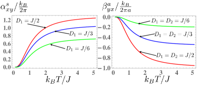
Figure 2: (Color online) Left: The spin Nernst conductivity $\alpha_{ij}^{s}$ versus temperature $T$ for DMI $D_{2}=0$ and $D_{1}=J/2$, $J/3$, and $J/6$. Right: The thermal torkance $\beta_{yx}^{a}$ corresponding to the anti-damping part of the torque versus temperature $T$ for DMI $D_{1}=D_{2}=J/2$, $J/3$, and $J/6$. Note that the temperature range is not limited by the Curie temperature in order to show the assymtotic behavior. In both figures the direction of the spin density is given by $\mathbf{m}=\hat{z}$.

Spin Nernst effect.— The thermal Hall effect manifests itself in the transverse temperature gradient Onose et al. (2010); Matsumoto et al. (2014); Mook et al. (2014). Here we calculate the transverse spin current which can be detected, e.g., via the inverse spin Hall effect in a Pt contact attached to the sample Saitoh et al. (2006). The spin Nernst conductivity $\alpha_{ij}^{s}$ relates the temperature gradient to the spin current density, i.e. $j_{i}^{s}=-\hbar j_{i}=-\alpha_{ij}^{s}\partial_{j}T$ where each magnon carries the angular momentum $-\hbar$. From Eq. (8) we obtain $\alpha_{ij}^{s}=t_{ij}/T$ with only the interband part contributing to $\alpha_{ij}^{s}$. For a model calculation, we consider Eq. (10). The spin Nernst effect can take place in systems with the center of inversion, thus the Rashba-like DMI described by parameter $D_{2}$ can be zero. By integrating the Berry curvature over the Brillouin zone, we arrive at the result in Fig. 2 where $\alpha_{ij}^{s}$ is dominated by the lowest band in Fig. 1 with the positive Chern number. For a three-dimensional system containing weakly interacting kagome layers, we can write $\alpha_{ij}^{\text{3D}}=\alpha_{ij}^{s}/c$ where $c\propto a$ is the interlayer distance and $a$ is the lattice constant. Given results in Fig. 2, it seems to be possible to generate a transverse spin current of the order of $10^{-10}\mbox{J}/\mbox{m}^{2}$ from a temperature gradient of $20\,\mbox{K}/\mbox{mm}$ Jiang et al. (2013) in three dimensional systems. Spin currents of such magnitude are typical for spin pumping experiments Weiler et al. (2013).

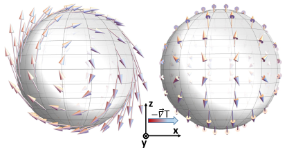
Figure 3: (Color online) The nonequilibrium magnon-mediated torque $\boldsymbol{\mathcal{T}}$ is plotted on a unit sphere representing the direction of uniform spin density $\mathbf{m}$. The temperature is $T=2J$ and the gradient is applied along the $-\hat{x}$ direction. The field-like torque component $\boldsymbol{\mathcal{T}}^{f}$ that is odd in the magnetization is plotted on the left and the anti-damping component $\boldsymbol{\mathcal{T}}^{a}$ that is even in the magnetization is plotted on the right. The field-like component is rescaled by the Gilbert damping to match in scale the anti-damping component, i.e., $\boldsymbol{\mathcal{T}}^{f}\rightarrow\alpha\boldsymbol{\mathcal{T}}^{f}$.

Nonequilibrium torques.— To present our results we introduce the thermal torkance $\beta_{ij}$ that relates the magnetization torque to the temperature gradient, i.e. $\mathcal{T}_{i}=-\beta_{ij}\partial_{j}T$ or $\beta_{ij}=m_{l}\varepsilon_{lki}t_{kj}/T$ in terms of Eq. (8) where $\varepsilon_{lki}$ is the antisymmetric tensor. We further separate the torkance $\beta_{ij}$ into the field-like part $\beta_{ij}^{f}$ that is odd in the magnetization and the anti-damping part $\beta_{ij}^{a}$ that is even in the magnetization.

To uncover the effect of Berry curvature, we apply our theory to the model in Eq. (10). Within our theory the anti-damping component of the torque entirely comes from the Berry curvature contribution in Eq. (8). The largest component of $\beta_{ij}^{a}$ corresponding to the temperature gradient along the $x-$axis, the torque along the $y-$axis, and the spin density along the $z-$axis is plotted in Fig. 2. The temperature dependence of $\beta_{ij}^{a}$ resembles the temperature dependence of the spin Nernst conductivity where we observe larger effect at higher temperatures. For a three-dimensional system containing weakly interacting kagome layers, we obtain $\beta_{ij}^{\text{3D}}=\beta_{ij}/c$ where $c$ is the interlayer distance. In Fig. 3, we plot the nonequilibrium magnon-mediated torque separated into the field-like and anti-damping parts, $\boldsymbol{\mathcal{T}}=\boldsymbol{\mathcal{T}}^{f}+\boldsymbol{\mathcal{T}}^{a}$, on a unit sphere representing the spin density vector $\mathbf{m}$. The torque in Fig. 3 can be obtained from phenomenological expressions obtained for films with structural asymmetry along the $z-$axis Manchon et al. (2014); Kovalev and Güngördü (2015), $\boldsymbol{\mathcal{T}}_{i}^{f}\propto(\mathbf{m}\times\mathbf{D}_{i})\partial_{i}T$ and $\boldsymbol{\mathcal{T}}_{i}^{a}\propto\mathbf{m}\times(\mathbf{m}\times\mathbf{D}_{i})\partial_{i}T$, by a deformation not involving the change in topology where $\mathbf{D}_{i}=\mathbf{e}_{z}\times\mathbf{e}_{i}$ and $i$ is either $x$ or $y$.

A ballpark estimate of the strength of the nonequilibrium magnon-mediated torque can be done by considering only the lowest band in the quadratic approximation, i.e., we have $H(\mathbf{k})=\hbar A[k_{\alpha}+\mathbf{m}\cdot(\mathbf{D}_{\alpha}/A-\boldsymbol{\cal{A}}_{\alpha})]^{2}/s$ where $A$ is the exchange stiffness, $\boldsymbol{\cal{A}}_{\alpha}$ is the texture-induced vector potential, $s$ is the spin density, and a tensor $D_{\alpha\beta}=\mathbf{D}_{\alpha}\cdot\mathbf{e}_{\beta}$ describes DMI. After substituting this spectrum in the first Eq. (8) we obtain the longitudinal spin current $\mathbf{j}^{s}=-\hbar\mathbf{j}=k_{B}\boldsymbol{\partial}T[\sqrt{\pi}\zeta(3/2)]/(8\pi^{2}\lambda\alpha)$ where $\zeta$ is the Riemann zeta function and $\lambda=\sqrt{\hbar A/sk_{B}T}$ is the thermal magnon wavelength. The same Eq. (8) results in the expression for the nonequilibrium field-like torque density:

$$\boldsymbol{\mathcal{T}}^{f}=[\mathbf{m}\times(\mathbf{D}_{\alpha}/A-\boldsymbol{\cal{A}}_{\alpha})]j_{\alpha}^{s},$$ (11)

which agrees with the earlier results obtained for a single-band ferromagnet Kovalev (2014); Manchon et al. (2014); Linder (2014); Kovalev and Güngördü (2015); Kim and Tserkovnyak (2015). Here the torque is generated within the whole volume. This is contrary to the conventional spin-transfer torque which is generated only close to the interface Kovalev et al. (2002). The typical charge current density $j^{e}=10^{10}\mbox{A}/\mbox{$m^{2}$}$ sufficient for the spin-transfer torque switching should be compared to $2ejdD/A\approx 10^{9}\mbox{A}/\mbox{$m^{2}$}$ where $e$ is the electron charge, $D$ is the strength of DMI and $d$ is the width of the magnet. For the estimate of the field-like torque, we assume that $d=A/D$, $\partial_{i}T=20\,\mbox{K}/\mbox{mm}$, and $\alpha=10^{-4}$ Jiang et al. (2013).

Conclusions.— We developed a linear response theory to temperature gradients for magnetization torques (DM torques). We identify the intrinsic part of the DM torque and express it through the Berry curvature. We note that similar expressions also arise for the magnon-mediated spin Nernst effect. According to our estimates, the spin Nernst effect leads to substantial spin currents that could be measured, e.g., by the inverse spin Hall techniques Saitoh et al. (2006) in such materials as pyrochlore crystals (e.g., Lu₂V₂O₇) and the kagome ferromagnets Hirschberger et al. (2015); Boldrin et al. (2015) [e.g., Cu(1-3, bdc)]. In particular, a voltage should arise in the neighboring heavy metal due to the inverse spin Hall effect in full analogy to measurements of the spin Seebeck effect and spin pumping Weiler et al. (2013). We also find that the DM torques should influence the magnetization dynamics in ferromagnets with DMI; however, larger temperature gradients (compared to $20\,\mbox{K}/\mbox{mm}$ used in estimates Jiang et al. (2013)) are required, e.g., for magnetization switching Pushp et al. (2015). For the validity of the linear response approximation the temperature should not change much over the magnon mean free path. The DM torque can only arise in materials with structural asymmetry or lacking the center of inversion. Of relevance could be jarosites Elhajal et al. (2002) or ferromagnets and ferrimagnets containing buckled kagome layers Pregelj et al. (2012); Rousochatzakis et al. (2015). Our theory can be readily generalized to antiferromagnets and ferrimagnets, extending the range of materials suitable for observation of DM torques. In particular, antiferromagnet does not have to have the center of inversion in order to exhibit the DM torque provided each sublattice individually lacks the center of inversion.

We gratefully acknowledge stimulating discussions with Kirill Belashchenko and Gen Tatara. This work was supported in part by the DOE Early Career Award DE-SC0014189, and by the NSF under Grants Nos. Phy-1415600, PHY11-25915, and DMR-1420645.

See pages ,1,,2,,3,,4,,5 of Supplementary5.pdf

References

- Žutić et al. (2004) I. Žutić, J. Fabian, and S. Das Sarma, Rev. Mod. Phys. 76, 323 (2004).
- Bauer et al. (2012) G. E. W. Bauer, E. Saitoh, and B. J. van Wees, Nat. Mater. 11, 391 (2012).
- Goennenwein and Bauer (2012) S. T. B. Goennenwein and G. E. W. Bauer, Nat. Nanotech. 7, 145 (2012).
- Weiler et al. (2013) M. Weiler, M. Althammer, M. Schreier, J. Lotze, M. Pernpeintner, S. Meyer, H. Huebl, R. Gross, A. Kamra, J. Xiao, et al., Phys. Rev. Lett. 111, 176601 (2013).
- Hatami et al. (2007) M. Hatami, G. E. W. Bauer, Q. Zhang, and P. J. Kelly, Phys. Rev. Lett. 99, 066603 (2007).
- Bauer et al. (2010) G. E. W. Bauer, S. Bretzel, A. Brataas, and Y. Tserkovnyak, Phys. Rev. B 81, 024427 (2010).
- Kovalev and Tserkovnyak (2009) A. A. Kovalev and Y. Tserkovnyak, Phys. Rev. B 80, 100408 (2009).
- Cahaya et al. (2014) A. B. Cahaya, O. A. Tretiakov, and G. E. W. Bauer, Appl. Phys. Lett. 104, 042402 (2014).
- Kovalev and Tserkovnyak (2010) A. A. Kovalev and Y. Tserkovnyak, Solid State Commun. 150, 500 (2010).
- Kovalev and Güngördü (2015) A. A. Kovalev and U. Güngördü, EPL (Europhysics Letters) 109, 67008 (2015).
- Kajiwara et al. (2010) Y. Kajiwara, K. Harii, S. Takahashi, J. Ohe, K. Uchida, M. Mizuguchi, H. Umezawa, H. Kawai, K. Ando, K. Takanashi, et al., Nature 464, 262 (2010).
- Onose et al. (2010) Y. Onose, T. Ideue, H. Katsura, Y. Shiomi, N. Nagaosa, and Y. Tokura, Science 329, 297 (2010).
- Uchida et al. (2010) K. Uchida, J. Xiao, H. Adachi, J. Ohe, S. Takahashi, J. Ieda, T. Ota, Y. Kajiwara, H. Umezawa, H. Kawai, et al., Nat. Mater. 9, 894 (2010).
- Torrejon et al. (2012) J. Torrejon, G. Malinowski, M. Pelloux, R. Weil, A. Thiaville, J. Curiale, D. Lacour, F. Montaigne, and M. Hehn, Phys. Rev. Lett. 109, 106601 (2012).
- Jiang et al. (2013) W. Jiang, P. Upadhyaya, Y. Fan, J. Zhao, M. Wang, L.-T. Chang, M. Lang, K. L. Wong, M. Lewis, Y.-T. Lin, et al., Phys. Rev. Lett. 110, 177202 (2013).
- Parkin et al. (2008) S. S. P. Parkin, M. Hayashi, and L. Thomas, Science 320, 190 (2008).
- Brataas et al. (2012) A. Brataas, A. D. Kent, and H. Ohno, Nat. Mater. 11, 372 (2012).
- Kim et al. (2015) S. K. Kim, S. Tewari, and Y. Tserkovnyak, Phys. Rev. B 92, 020412 (2015).
- Matsumoto and Murakami (2011) R. Matsumoto and S. Murakami, Phys. Rev. Lett. 106, 197202 (2011).
- Matsumoto et al. (2014) R. Matsumoto, R. Shindou, and S. Murakami, Phys. Rev. B 89, 054420 (2014).
- Katsura et al. (2010) H. Katsura, N. Nagaosa, and P. A. Lee, Phys. Rev. Lett. 104, 066403 (2010).
- Sundaram and Niu (1999) G. Sundaram and Q. Niu, Phys. Rev. B 59, 14915 (1999).
- Zhang et al. (2013) L. Zhang, J. Ren, J.-S. Wang, and B. Li, Phys. Rev. B 87, 144101 (2013).
- Mook et al. (2014) A. Mook, J. Henk, and I. Mertig, Phys. Rev. B 90, 024412 (2014).
- Mook et al. (2014) A. Mook, J. Henk, and I. Mertig, Phys. Rev. B 89, 134409 (2014).
- Hirschberger et al. (2015) M. Hirschberger, R. Chisnell, Y. S. Lee, and N. P. Ong, Phys. Rev. Lett. 115, 106603 (2015).
- Luttinger (1964) J. M. Luttinger, Phys. Rev. 135, 1505 (1964).
- Smrcka and Streda (1977) L. Smrcka and P. Streda, J. Phys. C 10, 2153 (1977).
- Qin et al. (2011) T. Qin, Q. Niu, and J. Shi, Phys. Rev. Lett. 107, 236601 (2011).
- Tatara (2015) G. Tatara, Phys. Rev. B 92, 064405 (2015).
- Moriya (1960) T. Moriya, Phys. Rev. 120, 91 (1960).
- Dzyaloshinsky (1958) I. Dzyaloshinsky, J. Phys. Chem. Solids 4, 241 (1958).
- Bernevig and Vafek (2005) B. A. Bernevig and O. Vafek, Phys. Rev. B 72, 033203 (2005).
- Manchon and Zhang (2008) A. Manchon and S. Zhang, Phys. Rev. B 78, 212405 (2008).
- Matos-Abiague and Rodríguez-Suárez (2009) A. Matos-Abiague and R. L. Rodríguez-Suárez, Phys. Rev. B 80, 094424 (2009).
- Chernyshov et al. (2009) A. Chernyshov, M. Overby, X. Liu, J. K. Furdyna, Y. Lyanda-Geller, and L. P. Rokhinson, Nat. Phys. 5, 656 (2009).
- Garate and MacDonald (2009) I. Garate and A. H. MacDonald, Phys. Rev. B 80, 134403 (2009).
- Endo et al. (2010) M. Endo, F. Matsukura, and H. Ohno, Appl. Phys. Lett. 97, 222501 (2010).
- Fang et al. (2011) D. Fang, H. Kurebayashi, J. Wunderlich, K. Výborný, L. P. Zârbo, R. P. Campion, A. Casiraghi, B. L. Gallagher, T. Jungwirth, and A. J. Ferguson, Nat. Nanotech. 6, 413 (2011).
- Liu et al. (2012) L. Liu, C.-F. Pai, Y. Li, H. W. Tseng, D. C. Ralph, and R. A. Buhrman, Science 336, 555 (2012).
- Kurebayashi et al. (2014) H. Kurebayashi, J. Sinova, D. Fang, A. C. Irvine, T. D. Skinner, J. Wunderlich, V. Novák, R. P. Campion, B. L. Gallagher, E. K. Vehstedt, et al., Nat. Nanotechnol. 9, 211 (2014).
- Garello et al. (2013) K. Garello, I. M. Miron, C. O. Avci, F. Freimuth, Y. Mokrousov, S. Blügel, S. Auffret, O. Boulle, G. Gaudin, and P. Gambardella, Nat. Nanotechnol. 8, 587 (2013).
- Kovalev and Tserkovnyak (2012) A. A. Kovalev and Y. Tserkovnyak, EPL (Europhysics Letters) 97, 67002 (2012).
- Géranton et al. (2015) G. Géranton, F. Freimuth, S. Blügel, and Y. Mokrousov, Phys. Rev. B 91, 014417 (2015).
- Qaiumzadeh et al. (2015) A. Qaiumzadeh, R. Â. A. Duine, and M. Titov, Phys. Rev. B 92, 014402 (2015).
- (46) See supplemental material for detailed derivations below.
- Freimuth et al. (2016) F. Freimuth, S. Blügel, and Y. Mokrousov, arXiv preprint arXiv:1602.03319 (2016).
- Saitoh et al. (2006) E. Saitoh, M. Ueda, H. Miyajima, and G. Tatara, Appl. Phys. Lett. 88, 182509 (2006).
- Manchon et al. (2014) A. Manchon, P. B. Ndiaye, J.-H. Moon, H.-W. Lee, and K.-J. Lee, Phys. Rev. B 90, 224403 (2014).
- Kovalev (2014) A. A. Kovalev, Phys. Rev. B 89, 241101 (2014).
- Linder (2014) J. Linder, Phys. Rev. B 90, 041412 (2014).
- Kim and Tserkovnyak (2015) S. K. Kim and Y. Tserkovnyak, Phys. Rev. B 92, 020410 (2015).
- Kovalev et al. (2002) A. A. Kovalev, A. Brataas, and G. E. Bauer, Phys. Rev. B 66, 224424 (2002).
- Boldrin et al. (2015) D. Boldrin, B. Fâk, M. Enderle, S. Bieri, J. Ollivier, S. Rols, P. Manuel, and A. S. Wills, Phys. Rev. B 91, 220408 (2015).
- Pushp et al. (2015) A. Pushp, T. Phung, C. Rettner, B. P. Hughes, S.-H. Yang, and S. S. P. Parkin, Proc Natl Acad Sci USA 112, 6585 (2015).
- Elhajal et al. (2002) M. Elhajal, B. Canals, and C. Lacroix, Phys. Rev. B 66, 014422 (2002).
- Pregelj et al. (2012) M. Pregelj, O. Zaharko, A. Günther, A. Loidl, V. Tsurkan, and S. Guerrero, Phys. Rev. B 86, 144409 (2012).
- Rousochatzakis et al. (2015) I. Rousochatzakis, J. Richter, R. Zinke, and A. A. Tsirlin, Phys. Rev. B 91, 024416 (2015).