Large Blue Spectral Isocurvature Spectral Index Signals Time-Dependent Mass

Abstract

We show that if a spectator linear isocurvature dark matter field degree of freedom has a constant mass through its entire evolution history, the maximum measurable isocurvature spectral index that is consistent with the current tensor-to-scalar ratio bound of about $r\lesssim 0.1$ is about $n_{I}\lesssim 2.4$, even if experiments can be sensitive to a $10^{-6}$ contamination of the predominantly adiabatic power spectrum with an isocurvature power spectrum at the shortest observable length scales. Hence, any foreseeable future measurement of a blue isocurvature spectral index larger than $\sim 2.4$ may provide nontrivial evidence for dynamical degrees of freedom with time-dependent masses during inflation. The bound is not sensitive to the details of the reheating scenario and can be made mildly smaller if $r$ is better constrained in the future.

I Introduction

Although minimal single-field slow-roll inflationary scenarios Starobinsky:1980te ; Sato:1980yn ; Linde:1981mu ; Mukhanov:1981xt ; Albrecht:1982wi ; Hawking:1982my ; Guth1982 ; Starobinsky:1982ee ; Bardeen:1983qw ; Freese:1990rb can successfully provide a dynamical explanation for the currently known features of the initial conditions in classical cosmological physics (e.g. the cosmic microwave background (CMB) Ade:2015xua ; Ade:2015lrj ; Ade:2013xsa ; Ade:2013lta ; Ade:2013rta ; Ade:2013sta ; Ade:2013ydc ; Keisler:2015hfa ; Hinshaw:2012fq ; Komatsu:2010fb ; Brown:2009uy ; Reichardt:2008ay ; Fowler:2010cy ; Lueker:2009rx ; Hikage:2012be and large scale structure Ross:2012sx ; Percival:2007yw ; Eisenstein:2005su ), it is natural to speculate that more than one single real field is dynamical during inflation. For such extra dynamical degrees of freedom not to spoil the flatness of the inflaton potential, it is also natural to assume that they are very weakly coupled to the inflaton (though this is obviously not a requirement). With this assumption, these extra dynamical degrees of freedom behave as spectators as far as the inflationary dynamics is concerned. If one of these dynamical degrees of freedom is taken to be a weakly interacting cold dark matter (CDM) field, then there exists a well-known observable called the CDM-photon isocurvature perturbations which becomes observable (e.g. Preskill:1982cy ; Abbott:1982af ; Dine:1982ah ; Axenides:1983hj ; Steinhardt:1983ia ; Turner:1983sj ; Linde:1984ti ; Turner:1985si ; Seckel:1985tj ; Kolb:1990vq ; Polarski:1994rz ; Gordon:2000hv ; Fox:2004kb ; Sikivie:2006ni ; Beltran:2006sq ; Hertzberg:2008wr ; Malik:2008im ; Langlois:2011zz ; Visinelli:2014twa ; Choi:2014uaa ; Kawasaki:2014una ; Harigaya:2015hha ; Kadota:2015uia ) if the CDM field is sufficiently weakly interacting and do not to thermalize.

There are two broad categories of scalar spectator field scenarios that can produce observable CDM-photon isocurvature perturbations: (i) linear spectators, such as axions Peccei:1977hh ; Weinberg:1977ma ; Wilczek:1977pj , and (ii) gravitationally produced superheavy dark matter scenarios, aka WIMPZILLAs Chung:1998zb ; Chung:1998ua ; Kuzmin:1999zk ; Kuzmin:1998kk ; Chung:2001cb ; Chung:1998bt (for some recent developments, see Aloisio:2015lva ; Fedderke:2014ura ; Chung:2013rda ; Chung:2013sla ). Linear spectator fields are characterized by having vacuum expectation values (VEVs) that are much larger than the amplitudes of their quantum fluctuations. The VEV oscillations generate the dark matter density in the universe today while the spatially inhomogeneous distribution of their energy-momentum tensors are determined by the quantum fluctuations. Such isocurvature fluctuations are called linear because the the energy-momentum tensor inhomogeneity is approximately linear in the fluctuations, in contrast with the the case of gravitationally produced superheavy dark matter scenarios. In this paper, we will focus on the linear spectator scenarios and will drop the “linear” adjective.

Scale-invariant isocurvature perturbations with negligible correlations with curvature perturbations are well constrained to be less than 3% of the adiabatic power Ade:2015lrj ; Ade:2013rta ; Hinshaw:2012fq ; Komatsu:2010in ; Valiviita:2009ck ; Sollom:2009vd ; Komatsu:2008ex ; Bean:2006qz ; Crotty:2003fp . However, isocurvature spectra with very blue spectral indices can be unobservably small on long wavelengths, for which the measurements are strongly constraining, but have large amplitudes on short wavelengths, where the measurements are less constraining Hikage:2008sk ; Takeuchi:2013hza ; Chung:2015pga . The case of a blue spectrum is qualitatively different from a “bump” in the spectrum because bumps usually involve a red part as well as a blue part, and because the blue spectrum here is envisioned to have a qualitatively extended $k$-space range over which an approximately constant blue spectral index persists.

One of the most natural models that can produce large blue CDM-photon isocurvature scenarios was given in Kasuya:2009up . This class of models is characterized by axions that have time-dependent masses due to the out-of-equilibrium nature of the Peccei-Quinn (PQ) symmetry breaking field. For constant mass linear spectator fields, large blue-spectral indices are difficult to produce in observably large amplitudes because the energy density of the VEV dilutes away. An intuitive perspective is that the closer the spectral index is to $n_{I}=1$ (scale invariant), the more the field fluctuations behave like a frozen VEV, while the closer the spectral index is to $n_{I}=4$, the more the field fluctuations behave as particles which can be diluted away by inflation.

Hence, a natural question, which is the subject of this paper, is what is the maximal measurable isocurvature spectral index that can be produced by a constant mass spectator field in the context of slow-roll inflationary scenarios where the adiabatic perturbation spectrum originates from the inflaton field fluctuations. For a linear spectator scenario, we find that the maximum measurable spectral index in the foreseeable future is about $n_{I}=2.4$ (where $n_{I}=1$ corresponds to scale invariance). Although measurability depends on the sensitivity of any given experiment, inflationary physics renders the dependence of the experimental sensitivity to be logarithmic (to obtain some intuition, see e.g. Eq. (50)). The bulk of this number originates from the ratio of the log of the dark matter density maximum enhancement due to the dark matter diluting as $a^{-3}$ (compared to radiation diluting as $a^{-4}$) and the number of efoldings necessary for the inflationary scenario to explain the observed homogeneity and isotropy of the universe. A better constraint on the inflationary tensor perturbation amplitude $r$ can decrease this number, but the sensitivity is only logarithmic. If restrictions are placed on the maximum reheating temperature, then the maximum measurable spectral index also decreases. We will illustrate this by assuming a perturbative reheating scenario and assuming that the gravitationally suppressed nonrenormalizable operators of dimension 5 or 6 are unavoidable.

The number 2.4 is interesting because there are claims in the literature Dent:2012ne ; Chluba:2013dna ; Sekiguchi:2013lma ; Takeuchi:2013hza that future experiments may be able to measure spectral indices of $n_{I}\gtrsim 3$. The results in this work demonstrate that if any of these experiments detect a blue isocurvature spectrum, then they may have uncovered evidence for a dynamical degree of freedom with a time-dependent mass.

Before proceeding, we note that the CDM-photon isocurvature observable that we focus on in this paper is distinct from the $\zeta$ correlator in the context of “heavy” masses discussed e.g. in Arkani-Hamed:2015bza ; Chen:2012ge ; Craig:2014rta and the $\zeta$-tensor correlators Dimastrogiovanni:2015pla which in some cases can also receive signatures from the isocurvature degrees of freedom. On the other hand, these works all include the common theme of secondary fields from inflation that can leave a blue spectral cosmological observable signature.

The order of presentation will be as follows. In Sec. II, we discuss the constraints considered in the spectral index maximization problem (there will turn out to be thirteen constraints). We then estimate the solution to the maximization problem analytically in Sec. III. Next, we solve the maximization problem numerically in Sec. IV. We then in Sec. V give a brief review of why the axionic models that naturally have time dependent masses can evade this bound and explain why this may be the most natural scenario to turn to if measurements are made of the spectral index that are larger than $\sim 2.4$. Finally, we summarize and discuss caveats in the conclusions.

II Maximization Problem

In this section, we define our class of models and the maximization problem at hand. In particular, we provide a definition of a measurable blue isocurvature spectral index for a real scalar field $\chi$ of constant mass that makes up a fraction $\omega_{\chi}$ of the total cold dark matter content through its background VEV oscillations, reminiscent of misaligned axion scenarios.

We consider effectively single-field slow-roll inflationary scenarios, in which adiabatic cosmological perturbations arise from the inflaton fluctuations. Here we define effectively single field to mean that a single field direction is important for the adiabatic inflationary observables. For example, hybrid inflation involves at least two fields, but during the slow-roll phase, only one field is dynamical as far as the adiabatic perturbations are concerned.

In this context, consider a linear spectator isocurvature field $\chi$ (see Chung:2015pga for a more precise definition) that is governed by the potential

$$V(\chi)=\frac{m^{2}}{2}\chi^{2},$$ (1)

in which $m$ is a constant. Writing $\chi=\chi_{0}(t)+\delta\chi(t,\vec{x})$, the background equation of motion on the metric $ds^{2}=dt^{2}-a^{2}(t)|d\vec{x}|^{2}$ is

$$\partial_{t}^{2}\chi_{0}+3H\partial_{t}\chi_{0}+m^{2}\chi_{0}=0,$$ (2)

in which as usual $H\equiv\dot{a}/a$. In accordance with the linear spectator definition, we assume that for the wave vector $k$ in the range of isocurvature observable of interest, we have

$$\chi_{0}(t_{k})\gg\frac{H(t_{k})}{2\pi},$$ (3)

in which $t_{k}$ is the time when the mode $k$ left the horizon (i.e. $k=a(t_{k})H(t_{k})$). The energy density in $\chi_{0}$ oscillations that remains today is assumed to be part of the total cold dark matter content. We can then divide the $\delta\chi$ (non-inflaton) perturbation into the adiabatic and non-adiabatic part in the Newtonian gauge as $\delta\chi_{k}=\delta\chi_{k}^{ad}+\delta\chi_{k}^{nad}$, in which the nonadiabatic classical isocurvature field fluctuation $\delta\chi_{k}^{nad}=h_{k}(t)$ obeys the equation

$$\ddot{h}_{k}+3H\dot{h}_{k}+m^{2}h_{k}=0$$ (4)

at the linearized level during inflation. If the approximate Bessel function solution index $\sqrt{9/4-m^{2}/H^{2}}$ is real while the modes are subhorizon, then the square root of the $\chi$-photon total isocurvature amplitude $\sqrt{\Delta_{s}^{2}(k)}$ is

$$\sqrt{\Delta_{s}^{2}(k)}\approx\omega_{\chi}\frac{\sqrt{k^{3}/(2\pi^{2})}2|h_{k}(t)|}{|\chi_{0}(t)|}$$ (5)

(we have assumed the usual Bunch-Davies normalization of $h_{k}\rightarrow 1/\sqrt{2k}$ in the limit of $k/(aH)\rightarrow\infty$), which remains frozen upon the horizon exit, where $\omega_{\chi}$ is the cold dark matter fraction constituted by $\chi$, assuming all of dark matter is cold. More precisely, the gauge invariant isocurvature spectrum is (in the notation of Chung:2015pga )

$$\sqrt{\Delta_{s}^{2}(k)}=\omega_{\chi}2\left(\frac{2^{\nu-\frac{1}{2}}|\Gamma(\nu)|}{\sqrt{\pi}}\right)\left(\frac{H(t_{k_{0}})/(2\pi)}{\chi_{0}(t_{k_{0}})}\right)\left(\frac{k}{k_{0}}\right)^{\frac{3}{2}-\nu+O(\epsilon_{k_{0}})},$$ (6)

in which

$$\nu=\frac{3}{2}\sqrt{1-\frac{4}{9}\frac{m^{2}}{H^{2}(t_{k_{0}})}},$$ (7)

in which $H(t_{k_{0}})$ is the expansion rate when the $k_{0}$ mode leaves the horizon. Hence, for the blue spectral indices that are of interest in this work, we have

$$n_{I}-1\approx 3-2\nu,$$ (8)

in which $\nu$ is a function of mass that also controls the time dependence of the background field $\chi_{0}$. This class of isocurvature perturbations will be uncorrelated with the curvature perturbations.

We will call $n_{I}-1\sim O(1)>0$ a large blue spectral index, which corresponds to $m/H(t_{k_{0}})\sim O(1)$. For the majority of this paper, we will take $k_{0}=k_{i}$, which labels the longest wavelength mode relevant for CMB observations (around $0.002$ Mpc^-1), and we will assume $50\epsilon_{k_{i}}\ll 4-n_{I}$. For brevity, we will also define $H_{i}\equiv H(t_{k_{i}})$.

As $\omega_{\chi}\propto\chi_{0}^{2}(t)$ in Eq. (6), and $\chi_{0}(t)$ decays exponentially during inflation whenever $m/H_{i}\sim O(1)$, $\Delta_{s}^{2}$ can easily become unmeasurably small for large blue spectral index scenarios. This suppression can be partially offset by $(k/k_{0})^{n_{I}-1}$ enhancements as long as

$$\mbox{constraint 1}:\,\,\,\sqrt{\Delta_{s}^{2}(k_{\rm max})}/\omega_{\chi}<1$$ (9)

to maintain perturbativity. In addition, $H_{i}$ cannot in general be made arbitrarily large to make $\Delta_{s}^{2}$ large due to model building constraints such as the minimum number of efolds, reheating, and tensor perturbation limits.

Given these constraints, a natural question arises:

• Given an experimental sensitivity parameterized by $E_{k_{max}}$ (which will be defined below), what is the maximum measurable $n_{I}$ that can be attributed to a constant mass spectator model in the context of effectively single-field inflation?

This is the main question that will be answered in this paper, and the rest of the constraints (together with Eq. (9)) associated with maximizing $n_{I}$ in Eq. (6) will be laid out in this section.

The main physics computation underlying this question is the determination of the time evolution of $\chi_{0}(t)$ until the time of reheating. The computation thus depends on the expansion rate $H(t)$ during and after inflation. More specifically, the $\chi_{0}(t)$ time dependence is governed by the time-coarse-grained amplitude of $H$ because Eq. (2) does not contain any derivatives of $H(t)$. To cover a large class of slow-roll models economically (including both hybrid type and chaotic type), we consider a coarse-grained model space parameterized by $H_{i}$ (the expansion rate when the the longest wavelength left the horizon), $\epsilon_{k_{i}}$ (the potential slow-roll parameter when the longest mode left the horizon), and $t_{e}-t_{k_{i}}$. More precisely, we parameterize the expansion rate as

$$H\approx\left\{\begin{array}[]{ccc}H_{i}(1-\epsilon_{k_{i}}H_{i}(t-t_{k_{i}}))&&t_{k_{i}}<t<t_{e}\\ \frac{H_{i}(1-\epsilon_{k_{i}}H_{i}(t_{e}-t_{k_{i}}))}{1+\frac{3}{2}(t-t_{e})H_{i}(1-H_{i}\epsilon_{k_{i}}(t_{e}-t_{k_{i}}))}&&t>t_{e}\end{array}\right.$$ (10)

which is continuous at $t_{e}$. We will consider $\epsilon_{k_{i}}$ values that are consistent with the single-field adiabatic perturbation amplitude

$$\mbox{constraint 2:}\,\,\,\,\,\,\epsilon_{k_{i}}(H_{i})=\frac{H_{i}^{2}}{8\pi^{2}M_{p}^{2}\Delta_{\zeta}^{2}(k_{i})},$$ (11)

in accordance with the spectator isocurvature paradigm considered in this paper. In the above, $\Delta_{\zeta}^{2}(k_{i})$ is the adiabatic spectral amplitude at the longest observable wavelengths, which we will take to be $\Delta_{\zeta}^{2}(k_{i})\approx 2.4\times 10^{-9}$. As we seek a conservative upper bound on $n_{I}-1$, we will not impose the adiabatic scalar spectral index constraint. The set of models that this parameterization excludes are those for which the quantities $\{\epsilon_{k_{i}},\,H_{i},\,t_{e}\}$ do not control $H(t_{e})$, the expansion rate at the end of inflation. Such excluded models are somewhat atypical among known set of explicit effectively single-field models as they require new length scales (i.e. beyond $H_{i}$ and $t_{e}$) to enter the potential beyond those that are typically present in hybrid and chaotic inflationary scenarios. Furthermore, new length scales require yet another degree of fine tuning to fit smoothly with the $t\sim t_{k_{i}}$ time region where Eq. (10) is guaranteed to be valid for effectively single-field slow-roll models. As we will discuss later, the maximum spectral index constraint does not sensitively depend on $\epsilon_{k_{i}}H_{i}t_{e}$, which is fortunate since this parameterization is only 40% accurate for quadratic inflationary models near the time of the end of inflation. Note also that because we will impose the tensor perturbation phenomenological upper bound on $H_{i}$, the $\epsilon_{k_{i}}$ contribution to the spectral index will never be too big for phenomenological compatibility.

In addition to the adiabatic constraint Eq. (11), we impose the inflationary condition that the number of efolds be larger than the minimum necessary for a successful cosmology:

$$\mbox{constraint 3:\,\,\,}N_{e}\equiv H_{i}\Delta t_{e}\left[1-\frac{\epsilon_{k_{i}}}{2}H_{i}\Delta t_{e}\right]>N_{min} \approx 53+\frac{1}{3}\ln\frac{T_{RH}}{10^{10}{\rm GeV}}-\frac{2}{3}\ln\frac{H_{e}(H_{i},t_{e})}{10^{10}{\rm GeV}},$$ (12)

in which

$$H_{e}\equiv H_{i}(1-\epsilon_{k_{i}}H_{i}(\Delta t_{e})),\qquad\Delta t_{e}\equiv t_{e}-t_{k_{i}},$$ (13)

and we have taken the largest length scale to be $k_{{\rm min}}\sim 2\pi H_{0}a_{0}$. Note that in writing Eq. (12), we are neglecting contributions of order $\ln\left(c_{h}H_{i}/(2H_{e})\right)$, in which $c_{h}$ is an inflationary model dependent function of order unity. This leads to a systematic uncertainty with approximately a 2% error in the isocurvature spectral index bound. Note also Eq. (12) is a non-linear constraint on $H_{i}$.

We also impose the constraint that arises from assuming that there is at least one gravitational strength operator that can reheat the universe. Such assumptions are well motivated within string-motivated cosmologies (e.g. Blumenhagen:2014gta ; Cicoli:2012cy ; Cicoli:2010ha ; Green:2007gs ; Chen:2006ni ; Chialva:2005zy ; Frey:2005jk ; Kofman:2005yz ) and the weak gravity conjecture ArkaniHamed:2006dz (for some recent developments, see e.g. Brown:2015iha ; Rudelius:2015xta ; Cheung:2014vva ), as well as generic expectations of interpreting gravity as an effective theory with the cutoff scale $M_{p}$. The minimum reheat temperature for a given $H_{e}$ can be computed assuming a coherent oscillation perturbative reheating. For the inflaton field degree of freedom $\varphi$ at the end of inflation to oscillate, we must have its mass $m_{\varphi}$ satisfy the condition $m_{\varphi}\gtrsim H_{e}$. If the particle decay is through a dimension $n_{\mathcal{O}}\geq 5$ operator, then

$$\Gamma_{g}\sim S\frac{m_{\varphi}^{2(n_{\mathcal{O}}-4)+1}}{M_{p}^{2(n_{\mathcal{O}}-4)}}$$ (14)

is the gravitational decay rate representing the “weakest” decay rate where $S$ is a phase space suppression factor. For 2-body decay, we expects $S\sim(8\pi)^{-1}$, and we will take $S$ as small as $(0.1)^{2}/(8\pi)$ to get a conservative bound. Since

$$T_{RH}=0.2\left(\frac{200}{g_{*}(T_{RH})}\right)^{1/4}\sqrt{\Gamma M_{p}},$$ (15)

in which $\Gamma$ is the total decay rate, the bound $\Gamma\gtrsim\Gamma_{g}$ and $m_{\varphi}\gtrsim H_{e}$ lead to the following bound

$$\mbox{constraint 4:\,\,\,\,\,\,}H_{e}\lesssim H_{e\mbox{ rh bound}}(T_{RH})\equiv\left[\left(\frac{T_{RH}}{0.2\left(\frac{200}{g_{*}(T_{RH})}\right)^{1/4}}\right)^{2}\frac{M_{p}^{2(n_{\mathcal{O}}-4)-1}}{S}\right]^{\frac{1}{2(n_{\mathcal{O}}-4)+1}}.$$ (16)

As we will see, for the maximal spectral index bounds at the highest reheating temperatures, this constraint is unimportant. A further constraint from reheating is that $\{H_{i},\epsilon_{k_{i}},t_{e}\}$ has to be chosen for a fixed reheating temperature such that the energy at the end of inflation is large enough to give the total radiation energy:

$$\mbox{constraint 5:\,\,\,\,\,\,}T_{RH}<\left(\frac{10}{g_{*}}\right)^{1/4}\sqrt{\frac{3}{\pi}M_{P}H_{e}}.$$ (17)

Here we have implicitly assumed $T_{RH}$ and $H_{e}$ are such that coherent oscillations of $\chi$ occurs during the oscillation period of the inflaton. This condition can be written as

$$\frac{3}{2}H(t_{RH})<m,$$ (18)

which can be used to put a lower bound on the spectral index of

$$\mbox{constraint 6:\,\,\,\,\,\,}n_{I}-1>3-\sqrt{9-\left[\frac{\pi^{2}}{10}g_{*}(T_{RH})\left(\frac{T_{RH}^{2}}{M_{p}H_{i}}\right)^{2}\right]}.$$ (19)

Although imposing constraint 6 seems artificial since it is a simplification for calculational and presentation purposes, the parametric region where this bound is relevant is very similar to the parametric region where constraint 5 is relevant (i.e., it excludes the similar $\{H_{i},t_{e}\}$ region). Hence, there is no qualitative change in computing the maximum $n_{I}-1$. Furthermore, we find in the explicit numerical work that $n_{I}-1$ bound is lowered through constraint 6 by less than 1% which is below the systematic uncertainty in the computation. Hence, constraint 6 is a posteriori not important as long as constraint 5 is imposed.

The absence of observed tensor perturbations yield the following phenomenological bound:

$$\mbox{constraint 7:\,\,\,\,\,\,}H_{i}<M_{p}\sqrt{\frac{r_{b}}{2}\Delta_{\zeta}^{2}(k_{i})}$$ (20)

in which $r_{b}$ is the bound on the tensor-to-scalar ratio (i.e. the ratio $r<r_{b}\simeq 16\epsilon_{k_{i}}$). For the dark matter fraction to not exceed unity, we impose another phenomenological bound of

$$\mbox{constraint 8:}\,\,\,\,\,\,\,\,\omega_{\chi}\leq 1.$$ (21)

We see that constraints $2-5$ and 7 mainly arise from inflationary model-building consistency, while constraint 8 deals with dark matter phenomenology.

We now turn to constraints on isocurvature perturbations in addition to constraints 1 and 6. Let us suppose that future experiments can detect isocurvature amplitudes $\sqrt{\Delta_{s\,o}^{2}(k_{\rm max})}$ above $E_{k_{\rm max}}\sqrt{\Delta_{\zeta}^{2}(k_{i})}$, in which $E_{k_{\rm max}}$ parameterizes the experimental sensitivity. Eq. (6) implies

$$\mbox{constraint 9: }\,\,\,\,\,\,\,\omega_{\chi}2\left(\frac{2^{\nu-\frac{1}{2}}|\Gamma(\nu)|}{\sqrt{\pi}}\right)\left(\frac{H_{i}/(2\pi)}{\chi_{0}(t_{k_{i}})}\right)\left(\frac{k_{\rm max}}{k_{i}}\right)^{\frac{3}{2}-\nu}\geq E_{k_{\rm max}}\sqrt{\Delta_{\zeta}^{2}(k_{i})},$$ (22)

in which we have assumed $3/2-\nu\gg\epsilon_{k_{i}}$. We note that neglecting $\epsilon_{k_{i}}$ in the spectral index is numerically valid to better than 2% level for the upper bound of interest.

To see that constraint 9 controls the bound on the isocurvature $n_{I}-1$ that we are seeking, we note that if $\chi_{0}$ oscillations occur before reheating, we have

$$\omega_{\chi}=\frac{m^{2}\langle\left(\chi_{0}\right)^{2}\rangle_{t=t_{RH}}\left(\frac{a(t_{RH})}{a(t_{eq})}\right)^{3}}{\rho_{R}(T_{eq})(\Omega_{DM}/(\Omega_{b}+\Omega_{DM}))},$$ (23)

in which $\Omega_{DM}$ is the total dark matter fraction of the critical density today, $\Omega_{b}$ is the total baryonic fraction today, and $t_{eq}$ is the time of matter-radiation equality. The prediction from the coherent oscillation perturbative reheating scenario takes the form

$$\omega_{\chi}=R\frac{2\langle\left(\chi_{0}\right)^{2}\rangle_{t=t_{RH}}}{M_{p}^{2}}\left[\frac{m}{H(t_{RH})}\right]^{2}\left(\frac{T_{RH}}{T_{eq}}\right),$$ (24)

in which

$$R\equiv\frac{\Omega_{b}+\Omega_{DM}}{\Omega_{DM}}\frac{1}{6}\frac{g_{*}(T_{RH})}{g_{*}(T_{eq})}\frac{g_{*S}(T_{eq})}{g_{*S}(T_{RH})}\approx\frac{\Omega_{b}+\Omega_{DM}}{\Omega_{DM}}\frac{3.94}{3.38}\frac{1}{6}\approx 0.23,$$ (25)

where $g_{*}(T)$ counts the degrees of freedom in the radiation energy density $\rho_{R}$, $g_{*S}(T)$ counts the degrees of freedom in the entropy density, and $T_{eq}\approx 0.8$ eV is the matter-radiation equality temperature. As the solution to Eq. (2) is approximately given by

$$\left(\chi_{0}(t)/\chi_{0}(t_{k_{i}})\right)^{2}\sim e^{-(n_{I}-1)H_{i}(t-t_{k_{i}})}$$ (26)

during inflation, while the next most important factor is

$$\left(\frac{k}{k_{i}}\right)^{\frac{3}{2}-\nu}=e^{\frac{n_{I}-1}{2}\ln\left(\frac{k}{k_{i}}\right)}$$ (27)

with $\ln[k/k_{i}]\ll$ (number of efolds of inflation), we see that the magnitude of the left hand side of constraint 9 is controlled by $\omega_{\chi}$ and will be monotonically decreasing as $(n_{I}-1)/2$ increases in the blue spectral parametric region of interest. Hence, we conclude that the maximum $n_{I}-1$ is obtained when we saturate the inequality of constraint 9.

It is also necessary to check the current phenomenological bound on the isocurvature perturbations:

$$\sqrt{\frac{\Delta_{s}^{2}(k_{1})}{\Delta_{\zeta}^{2}(k_{1})}}<E_{k_{1}},$$ (28)

in which the current phenomenological bound on $E_{k_{1}}$ for $k_{1}\approx 0.05$ Mpc^-1 is $\sim 0.2$ at 95% confidence level Ade:2015lrj . Since $\Delta_{s}^{2}(k)\propto k^{n_{I}-1}$, when constraint 9 is saturated Eq. (28) becomes

$$\frac{E_{k_{\rm max}}\sqrt{\Delta_{\zeta}^{2}(k_{i})}\left(\frac{k_{1}}{k_{\rm max}}\right)^{\frac{n_{I}-1}{2}}}{\sqrt{\Delta_{\zeta}^{2}(k_{1})}}<E_{k_{1}}.$$ (29)

To simplify the approximate phenomenological constraint parameterization, we choose $k_{1}=k_{i}$:

$$\mbox{constraint 10}:\,\,\,\,\,\,\,E_{k_{\rm max}}\left(\frac{k_{i}}{k_{\rm max}}\right)^{\frac{n_{I}-1}{2}}<E_{k_{i}}.$$ (30)

Finally, we must also make sure we are in the linear spectator regime with our choice of $k_{\rm max}$:

$$\mbox{constraint 11:}\,\,\,\,\,\,\,\,\chi_{0}(t_{k_{\rm max}})>\frac{H(t_{k_{\rm max}})}{2\pi}$$ (31)

and $\chi_{0}(t_{k_{i}})$ is not trans-Planckian:

$$\mbox{constraint 12:}\,\,\,\,\,\,\,\,\chi_{0}(t_{k_{i}})\leq M_{p}.$$ (32)

There is another uncertainty in constraint 9 that is associated with the fact that the Bessel function mode functions are not obviously accurate solutions whenever the slow-roll parameter is not negligible. The limitations due to this issue were spelled out in Chung:2015pga . A more accurate power-law expansion should have a fiducial value of $k_{0}=k_{\rm max}$ instead of $k_{i}$. (The price that is paid for doing this is a complicated/numerical expression for $\chi_{0}(t_{k_{\rm max}})$ in terms of $\chi_{0}(t_{k_{i}})\leq M_{p}$.) This will turn out to be an issue only for values of $H_{i}$ that saturate constraint 7 with $r_{b}\gg 10^{-2}$ because $m/H(t)$ evolves significantly in that case during inflation. To address this issue, for such worrisome situations we therefore check the following constraint numerically

$$\mbox{constraint 9': }\omega_{\chi}\frac{\sqrt{k^{3}/(2\pi^{2})}2|h_{k}(t_{k_{i}})|}{|\chi_{0}(t_{k_{i}})|}\geq E_{k_{\rm max}}\sqrt{\Delta_{\zeta}^{2}(k_{i})}$$ (33)

involving a more accurate set of numerical solutions only. Finally, we note that constraint 9 also assumes that

$$\mbox{constraint 13: \,\,\,\,\,\,\,\,\,\,\,}\frac{m}{H(t_{k_{\rm max}})}<\frac{3}{2},$$ (34)

since only the non-decaying mode has been kept. We will see that in practice this does not pose a significant constraint.

In summary, the problem of finding the maximally observable constant mass isocurvature spectral index $n_{I}$ for a given experimental sensitivity $E_{k}$ is to find the maximum $n_{I}$ that satisfies the constraints 1-13 given above.

III Analytic Estimate

In this section, we provide an analytical estimate of the solution to the $n_{I}-1$ extremization problem presented in Sec. II. We begin in Section III.1 by giving a crude estimate of the maximization problem that is obtained by neglecting the slow-roll parameter $\epsilon_{k_{i}}$. In Section III.2, we then obtain an analytic perspective of the effect of turning on the slow-roll evolution of $H$ and the non-linearities of the problem. For example, we will see that the $H_{i}$ may not quite saturate constraint 7 for the largest spectral index, in contrast with the estimate given in Section III.1, and this turns out to be significant for the accuracy of the approximation of the spectral index used in constraint 9. Sec. IV will involve a numerical solution to the constrained maximization problem without resorting to the analytic arguments presented in this section.

III.1 Without Slow-roll Evolution

As previously discussed, the maximal spectral index results when constraint 9 is saturated. To evaluate constraint 9, we need to determine $\langle\left(\chi_{0}\right)^{2}\rangle_{t=t_{RH}}$. In this section, we will estimate this quantity to obtain a qualitative understanding of the parameters involved.

Let us neglect the slow-roll evolution of $H$ and assume that $\chi_{0}$ coherently oscillates just at the end of inflation. We can then estimate

$$\langle\left(\chi_{0}\right)^{2}\rangle_{t=t_{RH}}\sim C\left[\frac{H(t_{RH})}{H(t_{e})}\right]^{2}$$ (35)

$$C\equiv\frac{1}{2}\chi_{0}^{2}(t_{k_{i}})\exp\left[-(n_{I}-1)N_{e}\right],$$ (36)

in which $N_{e}\approx H_{i}(t_{e}-t_{k_{i}})$ is the number of efolds of inflation. Through standard cosmological scaling, this yields the dark matter fraction to be

$$\omega_{\chi}\sim R\frac{\chi_{0}^{2}(t_{k_{i}})\exp\left[-(n_{I}-1)N_{e}\right]\left[\frac{m}{H_{i}}\right]^{2}}{M_{p}^{2}}\left(\frac{T_{RH}}{T_{eq}}\right).$$ (37)

Now, noting that $m/H_{i}\sim O(1)$, and that the greatest $n_{I}-1$ sensitivity comes from the exponential, we find (assuming constraint 1 is satisfied)

$$n_{I}-1 \lesssim \frac{55}{N_{e}\left(1-\frac{1}{2N_{e}}\ln\left[\frac{k_{max}}{k_{i}}\right]\right)}\left(1+\frac{1}{55}\ln\left[\frac{10^{-5}2\left(\frac{2^{\nu-\frac{1}{2}}|\Gamma(\nu)|}{\sqrt{\pi}}\right)\left(\frac{H_{i}/(2\pi)}{\chi_{0}(t_{k_{i}})}\right)}{E_{k_{\rm max}}\sqrt{\Delta_{\zeta}^{2}(k_{i})}}\left(\frac{T_{RH}}{10^{10}{\rm GeV}}\right)\right]\right.$$ (38)

$$\left.+\frac{1}{55}\ln\left[\frac{\left(\chi_{0}\right)_{t_{k_{min}}}^{2}R}{M_{p}^{2}}\right]\right),$$

in which we note that $\nu=(3-[n_{I}-1])/2$. Hence, we see that increasing $T_{RH}$, $k_{max}/k_{i}$, and $H_{i}$ while decreasing $N_{e}$ and $E_{k_{max}}$ is what we want to maximize $n_{I}$. Clearly, $N_{e}$ cannot be decreased beyond the minimal number of efolds $N_{min}$ that is necessary for a successful inflationary scenario (constraint 3) for a fixed $T_{RH}.$ This will be one of the strongest constraints for bounding $n_{I}-1$. Increasing $H_{i}$ while keeping $N_{e}$ (and $T_{RH}$) fixed requires decreasing $t_{e}$, since $N_{e}\sim H_{i}(t_{e}-t_{k_{i}})$. However, because $N_{min}$ also changes if $H_{i}$ and $t_{e}$ changes, it is not possible to keep $N_{e}$ fixed right at the constraint boundary. As $H_{i}$ keeps increasing, it eventually runs into the tensor perturbation constraint 7. Also relevant for the case of low reheating temperatures is the fact that for sufficiently large $H_{i}/T_{RH}$, we run into constraint 4. For each $T_{RH}$, $n_{I}-1$ can be maximized through the $H_{i}$ and $t_{e}$ variations subject to the constraints just described.

As $T_{RH}$ is increased towards the highest temperatures consistent with energy conservation, constraints 5 and 6 become relevant. Even though constraint 6 is a tiny bit stronger of a constraint, it is very similar in numerical value to constraint 5. This is fortunate because as described before, constraint 6 is imposed for computational convenience and constraint 5 arises from fundamental principle of energy conservation. In the $\{H_{i},t_{e}\}$ parametric region where constraints 5 and 6 compete, the reheating scenario is somewhat unrealistic in that the reheating time scale is very fast, taking the system away from the coherent oscillation perturbative reheating regime. However, to put a conservative upper bound, we account for this extreme parametric region as well. It is in this sense that the bound that we will obtain for the maximum $n_{I}$ is reheating scenario independent.

We next note that for lower reheating temperatures satisfying constraint 7

$$H_{e\mbox{ rh bound}}(T_{RH})<M_{p}\sqrt{\frac{r}{2}\Delta_{\zeta}^{2}}$$ (39)

(with $H_{i}$ maximized to maximize $n_{I}-1$), $H_{i}$ has to be brought down when $T_{RH}$ is brought down to satisfy constraint 4:

$$H_{i}\sim\left[\left(\frac{T_{RH}}{0.2\left(\frac{200}{g_{*}(T_{RH})}\right)^{1/4}}\right)^{2}\frac{M_{p}^{2(n_{\mathcal{O}}-4)-1}}{S}\right]^{\frac{1}{2(n_{\mathcal{O}}-4)+1}}.$$ (40)

Since we have saturated constraint 9, we see that

$$\omega_{\chi}=\frac{E_{k_{\rm max}}\sqrt{\Delta_{\zeta}^{2}(k_{i})}}{2\left(\frac{2^{\nu-\frac{1}{2}}|\Gamma(\nu)|}{\sqrt{\pi}}\right)\left(\frac{H_{i}/(2\pi)}{\chi_{0}(t_{k_{i}})}\right)\left(\frac{k_{max}}{k_{i}}\right)^{\frac{3}{2}-\nu}}$$ (41)

increases as $H_{i}$ is lowered. Hence, depending in particular on the numerical values of $E_{k_{\rm max}}$ and $k_{max}/k_{i}$, the required $\omega_{\chi}$ can exceed unity, violating constraint 8.

Finally, if we choose $k_{i}/k_{\rm max}\lesssim 10^{-5}$ and $E_{k_{i}}/E_{k_{\rm max}}\gtrsim 3\times 10^{-3}$, we can always satisfy constraint 10 if $n_{I}-1\sim 1$. The current scale invariant isocurvature perturbation bound is given by

$$\frac{\Delta_{s}^{2}(100k_{i})}{\Delta_{\zeta}^{2}(100k_{i})}\lesssim 3\times 10^{-2}.$$ (42)

If this scale invariant spectrum bound is assumed to bound the blue spectrum as well, we have

$$E_{k_{i}}\sim\sqrt{3\times 10^{-2}\times 10^{-2}}\sim 10^{-2}$$ (43)

for $n_{I}-1\sim 1$. Hence, we see that if we choose $E_{k_{\rm max}}\lesssim 1$ and $k_{i}/k_{\rm max}\lesssim 10^{-5}$ , we can satisfy constraint 10. Therefore, we will focus on this parametric regime and ignore constraint 10.

Let us now find an explicit estimate of the largest value of $n_{I}$. First, we consider the case of

$$T_{RH}>T_{n_{\mathcal{O}}}$$ (44)

$$T_{n_{\mathcal{O}}}\equiv 2^{\frac{5}{2}-\frac{n_{\mathcal{O}}}{2}}\left(\Delta_{\zeta}^{2}\right)^{\frac{n_{\mathcal{O}}}{2}-\frac{7}{4}}M_{p}r^{-\frac{7}{4}+\frac{n_{\mathcal{O}}}{2}}\sqrt{\frac{S}{5\sqrt{g_{*}(T_{RH})}}}\approx\begin{cases}2\times 10^{10}r^{3/4}\sqrt{S8\pi}{\rm GeV}&\,\,\,\,\,\,\,\,\,n_{\mathcal{O}}=5\\ 6.8\times 10^{5}r^{5/4}\sqrt{S8\pi}{\rm GeV}&\,\,\,\,\,\,\,\,\,n_{\mathcal{O}}=6,\end{cases}$$ (45)

for which constraint 7 becomes relevant. Saturating constraints 3 and 7 in the current approximation scheme, we find

$$N_{e}\sim 52.8+\frac{1}{3}\ln\frac{T_{RH}}{10^{10}{\rm GeV}}-\frac{2}{3}\ln\frac{M_{p}\sqrt{\frac{r}{2}\Delta_{\zeta}^{2}}}{10^{10}{\rm GeV}}.$$ (46)

Although $T_{RH}$ appears here suggesting $T_{RH}$ should be minimized to maximize the $n_{I}-1$ bound, the $T_{RH}$ dependence shown explicitly in Eq. (38) dominates. As constraints 5 and 6 are similar in magnitude, we use constraint 5 to maximize $T_{RH}$ for simplicity for this simplified analytic estimate. In other words, here we estimate

$$\mbox{max }T_{RH} \approx \left(\frac{10}{g_{*}}\right)^{1/4}M_{p}\sqrt{\frac{3}{\pi}\sqrt{\frac{r}{2}\Delta_{\zeta}^{2}}}$$ (47)

$$\sim 6.5\times 10^{15}r^{1/4}\mbox{ GeV },$$ (48)

in which we have taken $g_{*}=200$ and $\Delta_{\zeta}^{2}(k_{i})=2.4\times 10^{-9}$. From Eq. (38), we then find that

$$n_{I}-1|_{T_{RH}=\mbox{max}T_{RH}} \lesssim \frac{55}{N_{e}^{est}\left(1-\frac{1}{2N_{e}^{est}}\ln\left[\frac{k_{max}}{k_{i}}\right]\right)}\left(1+\frac{1}{55}\ln\left[\frac{\left(\chi_{0}\right)_{t_{k_{min}}}^{2}R}{M_{p}^{2}}\right]\right.$$ (49)

$$\left.\frac{1}{55}\ln\left[\frac{4.2\times 10^{3}\left(\frac{2^{\nu-\frac{5}{4}}|\Gamma(\nu)|}{\pi^{2}}\right)\left(\frac{M_{p}}{\chi_{0}(t_{k_{i}})}\right)r^{3/4}}{E_{k_{\rm max}}}\left(\frac{10}{g_{*}}\Delta_{\zeta}^{2}(k_{i})\right)^{1/4}\right]\right)$$

$$\approx \boxed{\frac{1.2\times\left(1+\frac{1}{54}\ln\left[\frac{r^{3/4}}{E_{k_{\rm max}}}\right]\right)}{1-5.5\times 10^{-3}\ln r-1.1\times 10^{-2}\ln\left[\frac{k_{max}}{k_{i}}10^{-5}\right]}},$$ (50)

in which we have taken $g_{*}$ and $\Delta_{\zeta}^{2}(k_{i})$ to have the same numerical values as above. We have also taken $\chi_{0}(t_{k_{i}})=M_{p}$ to satisfy constraint 12, we have approximated $n_{I}-1\approx 1$ on the right hand side, and we used

$$N_{e}^{est}=52.8+\frac{1}{3}\ln\frac{\left(\frac{10}{g_{*}}\right)^{1/4}M_{p}\sqrt{\frac{3}{\pi}\sqrt{\frac{r}{2}\Delta_{\zeta}^{2}(k_{i})}}}{10^{10}{\rm GeV}}-\frac{2}{3}\ln\frac{M_{p}\sqrt{\frac{r}{2}\Delta_{\zeta}^{2}(k_{i})}}{10^{10}{\rm GeV}}\approx 51.2\left(1-\frac{\ln r}{205}\right).$$ (51)

We see that there is only a very mild dependence on the phenomenological parameterizations used above. Hence, if a blue isocurvature spectral index $n_{I}\gtrsim 3$ is measured, this certainly cannot arise from a linear spectator with a time-independent mass. We will sharpen this estimate with a numerical analysis in Sec. IV.

We next consider the case of

$$T_{n_{\mathcal{O}}}\lesssim T_{RH}\lesssim\left(\frac{10}{g_{*}}\right)^{1/4}M_{p}\sqrt{\frac{3}{\pi}\sqrt{\frac{r}{2}\Delta_{\zeta}^{2}(k_{i})}}\approx 6.5\times 10^{15}r^{1/4}{\rm GeV}$$ (52)

but still with $H_{i}$ saturating constraint 7:

$$\boxed{\begin{array}[]{ccc}n_{I}-1&\lesssim&\frac{1.06}{1-8\times 10^{-3}\ln r+8\times 10^{-3}\ln\frac{T_{RH}}{10^{11}{\rm GeV}}-1.2\times 10^{-2}\ln\left[\frac{k_{max}}{k_{i}}10^{-5}\right]}\times\\ &&\left(1+\frac{1}{44}\ln\left[\frac{\sqrt{r}}{E_{k_{\rm max}}}\right]+\frac{1}{44}\ln\frac{T_{RH}}{10^{11}{\rm GeV}}\right)\end{array}}$$ (53)

where we have used

$$N_{e}^{est}\approx 47.5-\frac{1}{3}\ln r+\frac{1}{3}\ln\frac{T_{RH}}{10^{11}{\rm GeV}}.$$ (54)

We can continue to lower the temperature towards $T_{n_{\mathcal{O}}}$ unless constraint 8 is saturated. Constraint 8 is saturated before reaching $T_{n_{\mathcal{O}}}$ if $n_{I}-1$ is smaller than the solution $n_{I}^{c}(T>T_{n_{\mathcal{O}}})-1$ to

$$\frac{2^{\frac{n_{I}^{c}-1}{2}-1}\chi_{0}(t_{k_{i}})\sqrt{\Delta_{\zeta}^{2}(k_{i})}E_{k_{\rm max}}\left(\frac{k_{\rm max}}{k_{{\rm min}}}\right)^{-\frac{(n_{I}^{c}-1)}{2}}\pi^{3/2}}{\kappa\sqrt{r}\Gamma\left(\frac{3-(n_{I}^{c}-1)}{2}\right)}=1,$$ (55)

which for $\{E_{k_{\mbox{max }}}=1,k_{\rm max}/k_{\mbox{min }}=10^{5},\chi_{0}(t_{k_{i}})=M_{p},r_{b}=10^{-3}\}$ is approximately $0.7$.

Let us now consider the lower reheating temperature $T_{RH}<T_{n_{\mathcal{O}}}$ (and $n_{I}-1>n_{I}^{c}-1$), which means that we should set

$$H_{i}\approx H_{e\mbox{ rh bound}}(T_{RH})$$ (56)

in Eq. (38) instead of using constraint 7. We find

$$\boxed{n_{I}-1\lesssim\begin{cases}\frac{1.06\left(1-0.023\ln\left[E_{k_{\rm max}}\right]+0.038\ln\frac{T_{RH}}{10^{11}{\rm GeV}}-7.6\times 10^{-3}\ln\left[S8\pi\right]\right)}{1+5.4\times 10^{-3}\ln\left[S8\pi\right]-2.7\times 10^{-3}\ln\frac{T_{RH}}{10^{11}{\rm GeV}}-1.2\times 10^{-2}\ln\left[\frac{k_{max}}{k_{i}}10^{-5}\right]}&\,\,\,\,\,\,\,\,\,n_{\mathcal{O}}=5\\ \frac{1.2\left(1-0.021\ln\left[E_{k_{\rm max}}\right]+0.030\ln\frac{T_{RH}}{10^{11}{\rm GeV}}-4.2\times 10^{-3}\ln\left[S8\pi\right]\right)}{1+3.5\times 10^{-3}\ln\left[S8\pi\right]+1.7\times 10^{-3}\ln\frac{T_{RH}}{10^{11}{\rm GeV}}-1.3\times 10^{-2}\ln\left[\frac{k_{max}}{k_{i}}10^{-5}\right]}&\,\,\,\,\,\,\,\,\,n_{\mathcal{O}}=6\end{cases}}$$ (57)

At lower $T_{RH}$, we have $\omega_{\chi}\gtrsim 1$ at

$$T_{DM2}=\begin{cases}\frac{4.6\times 10^{7}\mbox{ GeV }E_{k_{\rm max}}^{3/2}\sqrt{8\pi S}}{\left(\frac{k_{\rm max}/k_{{\rm min}}}{10^{5}}\right)^{3/4}}\left(1-(n_{I}-2)\left[8.5+\frac{3}{4}\ln\left(\frac{k_{\rm max}/k_{{\rm min}}}{10^{5}}\right)\right]\right)&\,\,\,\,\,\,\,\,\,\,\,\,\,\,\,\,\,n_{\mathcal{O}}=5\\ \frac{28\mbox{ GeV }E_{k_{\rm max}}^{5/2}\sqrt{8\pi S}}{\left(\frac{k_{\rm max}/k_{{\rm min}}}{10^{5}}\right)^{5/4}}\left(1-(n_{I}-2)\left[14+\frac{5}{4}\ln\left(\frac{k_{\rm max}/k_{{\rm min}}}{10^{5}}\right)\right]\right)&\,\,\,\,\,\,\,\,\,\,\,\,\,\,\,\,\,n_{\mathcal{O}}=6.\end{cases}$$ (58)

We have taken the minimum $T_{RH}$ in this paper to be at 100 GeV to simplify the presentation. This means that $\omega_{\chi}\lesssim 1$ constraint is more relevant for $n_{\mathcal{O}}=5$ case than the $n_{\mathcal{O}}=6$ case.

We should also estimate the effect of constraint 11 on $k_{\rm max}$:

$$\frac{k_{\rm max}}{k_{i}}\lesssim\left(\frac{\chi_{0}(t_{k_{i}})}{H_{i}/2\pi}\right)^{\frac{2}{n_{I}-1}},$$ (59)

which becomes

$$\frac{k_{\rm max}}{k_{i}}\lesssim 10^{8}$$ (60)

with $\chi_{0}(t_{k_{i}})=M_{p},$ $n_{I}-1=1.3$, and $H_{i}$ set at $r_{b}=0.1$.

Finally, constraint 13 can be shown to be generically satisfied in the $n_{I}-1$ and $k_{\rm max}/k_{\mbox{min }}$ region of interest. This will be discussed more in the numerical section below.

III.2 Perturbative in Slow-roll Evolution

In this subsection, we examine the effect of turning on $\epsilon_{k_{i}}$. We will see its most important feature is to have $n_{I}$ maximized for $|H_{i}-H_{e}|/H_{e}\ll 1$, making the Bessel spectral formula accurate.

Instead of completely neglecting $\epsilon_{k_{i}}$ during inflation in computing $\langle\left(\chi_{0}\right)^{2}\rangle_{t=t_{RH}},$ we can use linear perturbation theory in $\epsilon_{k_{i}}$ to solve Eq. (2) (for more details, see appendix A ):

$$\langle\left(\chi_{0}\right)^{2}\rangle_{t\geq t_{m},t_{e}}\sim\frac{\mathcal{A}}{2}\chi_{0}^{2}(t_{k_{i}})\exp\left[-(3-2\nu_{k_{i}})H_{i}(t_{e}-t_{k_{i}})\right]\left[\frac{H(t)}{H(t_{e})}\right]^{2}$$ (61)

$$\mathcal{A}\equiv\left(1-\frac{6(3-2\nu_{k_{i}})F_{1}\epsilon_{k_{i}}H_{i}\nu_{k_{i}}(t_{e}-t_{k_{i}})}{16\nu_{k_{i}}^{3}-3(3-2\nu_{k_{i}})\epsilon_{k_{i}}}\right)^{2}\left(1+F_{2}^{2}\right)$$ (62)

$$F_{1}\equiv H_{i}\nu_{k_{i}}(t_{e}-t_{k_{i}})-1$$ (63)

$$F_{2}\equiv\frac{32\nu_{k_{i}}^{4}+6\epsilon_{k_{i}}\nu_{k_{i}}\left\{3-2\nu_{k_{i}}\left[1+H_{i}(t_{e}-t_{k_{i}})\left(3+\nu_{k_{i}}[2+(3-2\nu_{k_{i}})H_{i}(t_{e}-t_{k_{i}})]\right)\right]\right\}+F_{3}}{\sqrt{9-4\nu_{k_{i}}^{2}}\left(16\nu_{k_{i}}^{3}-3\epsilon_{k_{i}}(3-2\nu_{k_{i}})(1+2F_{1}H_{i}\nu_{k_{i}}(t_{e}-t_{k_{i}})\right)}$$ (64)

$$F_{3}\equiv 9(3-2\nu_{k_{i}})\epsilon_{k_{i}}^{2}H_{i}(t_{e}-t_{k_{i}})[1+2F_{1}H_{i}\nu_{k_{i}}(t_{e}-t_{k_{i}})],$$ (65)

in which $t_{m}$ is the time after $\chi$ field starts to oscillate and $t_{e}$ is the end of inflation:

$$m=\frac{3}{2}H(t_{m}).$$ (66)

This allows us to rewrite the analog of Eq. (38) as

$$n_{I}-1\lesssim\frac{55}{N_{min}^{\prime}}\left(1+\frac{1}{55}\ln\left[\frac{10^{-5}}{\omega_{\chi\,{\rm min}}(n_{I}-1)}\left(\frac{T_{RH}}{10^{10}{\rm GeV}}\right)\right]+\frac{1}{55}\ln\left[\frac{\left(\chi_{0}\right)_{t_{k_{min}}}^{2}r_{m}^{2}(n_{I}-1)R}{M_{p}^{2}}\right]\right),$$ (67)

in which

$$N_{min}^{\prime}\approx\frac{1-\sqrt{1-2\epsilon_{k_{i}}N_{min}}}{\epsilon_{k_{i}}}$$ (68)

$$\omega_{\chi\,{\rm min}}(n_{I}-1)\equiv\mbox{max}\left[E_{k_{\rm max}}\sqrt{\Delta_{\zeta}^{2}(k_{min})},\frac{E_{k_{\rm max}}\sqrt{\Delta_{\zeta}^{2}(k_{min})}}{\sqrt{\Delta_{s}^{2}(k_{\rm max})}/\omega_{\chi}}\right]$$ (69)

$$r_{m}(n_{I}-1)\equiv\frac{m}{H_{i}(1-\epsilon_{k_{i}}N_{min}^{\prime})}\sqrt{\mathcal{A}},$$ (70)

$N_{min}$ is given by Eq. (12) $\mathcal{A}$ is given by Eq. (62), $\sqrt{\Delta_{s}^{2}(k_{\rm max})}/\omega_{\chi}$ is given by Eq. (6), and

$$\frac{m}{H_{i}}\approx\frac{1}{2}\sqrt{(n_{I}-1)(6-[n_{I}-1])}.$$ (71)

Comparing with Eq. (38), we see a complicated function $r_{m}(n_{I}-1)$ that depends on $n_{I}-1$. Most of this complicated function accounts for the $\epsilon_{k_{i}}$ dependence of the time evolution of $\chi_{0}(t)$.

When accounting for $\epsilon_{k_{i}}$ and constraint 2, we note that a given pair $H_{e}$ and $N_{e}$ can originate from two different values $H_{i}$:

$$H_{i}=\frac{\sqrt{\Delta_{\zeta}^{2}}M_{p}\sqrt{2\pi}\sqrt{\pi\pm\sqrt{\pi^{2}-\frac{H_{e}^{2}N_{e}}{M_{p}^{2}\Delta_{\zeta}^{2}}}}}{\sqrt{N_{e}}}.$$ (72)

With $H_{e}^{2}N_{e}\ll\pi^{2}M_{p}^{2}\Delta_{\zeta}^{2}$, the hybrid inflation case corresponds to the minus sign branch while the quadratic inflation case corresponds to the positive sign branch. One can also easily show that for the parametric regime of interest, $H_{e}$ never becomes close to zero even though there may be a worry from the form of Eq. (10) that we may be unreasonably extrapolating the linear expansion of the slow-roll that is valid near $t_{k_{i}}$. On the other hand, the parametric regions where the hybrid inflation and quadratic inflation branches merge are sensitive to the branchpoint singularity there.

The most important feature of turning on $\epsilon_{k_{i}}$ is that since now (with constraint 2 imposed)

$$N_{e}=\frac{4\pi^{2}\Delta_{\zeta}^{2}M_{p}^{2}}{H_{i}^{2}}\left(\frac{H_{i}^{2}}{H_{e}^{2}}-1\right),$$ (73)

the minimization of $N_{e}$ that is important for the extremization of $n_{I}-1$ (e.g. see Eq. (38) which in turn is related to constraint 9) gives a numerical pressure in the non-linear extremization problem to make $H_{i}$ close to $H_{e}$. This favors a smaller $\epsilon_{k_{i}}$ (in turn favoring small $H_{i}$) which competes with the pressure to extremize $H_{e}$ (favoring a large $H_{i}$) that arises from constraint 3. Hence, depending on the size of $r$, $H_{i}$ may not quite saturate constraint 7 as was done in the derivation of Eq. (50). This means that with $\epsilon_{k_{i}}$ turned on, the sensitivity to the tensor-to-scalar ratio $r$ entering constraint 7 is reduced for values of $r$ that are “large”. As we will see in Sec. IV, this makes the approximate spectral index Eq. (8) more accurate for $r_{b}=0.1$.

A figure of validity for the $\epsilon_{k_{i}}$ perturbations can be written as

$$C_{pert}\equiv\epsilon_{k_{i}}N_{e}^{2},$$ (74)

since the background field evolution equation during inflation

$$\partial_{t}^{2}\chi_{0}+3H_{i}(1-\epsilon_{k_{i}}H_{i}(t-t_{k_{i}}))\partial_{t}\chi_{0}+m^{2}\chi_{0}=0$$ (75)

has a secular term $\epsilon_{k}H_{i}(t-t_{k_{i}})$, and this term is integrated over a time period of $t_{e}-t_{k_{i}}\propto N_{e}$. Since $N_{e}\sim 50$, high $H_{i}$ models where $\epsilon_{i}$ approaches the tensor-to-scalar ratio $r$ bound have $C_{pert}$ approaching unity, and hence they cannot be addressed reliably using this perturbative approach. In the next section, we will turn to a numerical analysis of this extremization problem, which will allow us to get a handle on situations such as these when perturbative methods fail.

IV Numerical Results

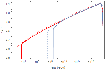
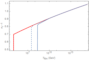
Figure 1: The maximum measurable spectral index $n_{I}-1$ assuming $\{E_{k_{\rm max}}=1,\,k_{\rm max}/k_{{\rm min}}=10^{5};\,r_{b}=10^{-1},10^{-3};\,n_{\mathcal{O}}=5,6;\,S=(8\pi)^{-1},10^{-2}(8\pi)^{-1}\}$ is plotted as a function of $T_{RH}$. (left) The bound on the tensor to scalar ratio $r_{b}$ has been taken to be $10^{-1}$. The maximum spectral index with the amplitude parameterized by $\{E_{k_{\rm max}}=1,\,k_{\rm max}/k_{{\rm min}}=10^{5}\}$ is around $n_{I}=2.11$. For $T\lesssim 10^{9}$ GeV, the lower solid curve corresponds to the reheating non-nonrenormalizable operator dimension of $n_{\mathcal{O}}=5$ while the upper solid curve corresponds to the case of the non-nonrenormalizable decay operator dimension of $n_{\mathcal{O}}=6$. For $T\gtrsim 10^{9}$ GeV, the two curves merge. The dashed curve corresponds to weakening the coefficient of the non-nonrenormalizable operator by a factor of 10. The vertical curve on the left portion of the boundary curves occur because the expansion rate there is too small in that parametric regime to produce measurable isocurvature perturbations (i.e. constraint 8). The dotted curve corresponds to evaluation of fiducial spectral index at $k_{\rm max}$ instead of $k_{{\rm min}}$. The correction is small (except at the highest $T_{RH}$ where the dip occurs) because constraint 7 is not saturated for $r_{b}=0.1$. (right) Similar to the left plot except with a probably possible future bound of $r_{b}=10^{-3}$.

In this section, we perform a numerical analysis to find the largest $n_{I}$ consistent with constraints 1 through 13. The results of this analysis will show that even with an extremely optimistic experimental sensitivity of $10^{-6}\Delta_{\zeta}^{2}$ on length scales as small as 10 kpc scales, the theoretical prediction from a constant mass isocurvature field scenario is that experiments will not measure spectral indices $n_{I}$ greater than $2.4$.

We begin with Fig. 1, which shows the case in which $\{E_{k_{\rm max}}=1,\,k_{\rm max}/k_{{\rm min}}=10^{5};\,r_{b}=10^{-1},10^{-3};\,n_{\mathcal{O}}=5,6;\,S=(8\pi)^{-1},10^{-2}(8\pi)^{-1}\}$. The results show that the maximum temperature estimated in Eq. (48) agrees with the right end of each plot to better than 30% and the maximum $n_{I}-1$ agrees with Eq. (50) to better than 5%. For the $r_{b}=0.1$ plot (the left plot), the reason why there is a drop of $n_{I}-1$ near $T_{RH}\sim 5\times 10^{15}$ GeV is due to constraint 5 (reheating energy conservation at time $t_{e}$) pushing up $H_{i}$ as $T_{RH}$ is raised. This upward push of $H_{i}$ is allowed because from the discussion around Eq. (73), constraint 7 may not be saturated depending on the size of $r.$ This non-saturation is indeed the case for most of the $r_{b}=0.1$ curve (which we have also checked directly numerically) and makes the approximate spectral index Eq. (8) more accurate. We see how the dotted curve matches the solid curve except at the highest temperature where the dip occurs, as we will discuss more below. For the $r_{b}=10^{-3}$ case, constraint 7 does saturate at the highest allowed reheating temperature, which means that no upward push of $H_{i}$ ever arises from constraint 5 for these highest temperatures. The maximum $n_{I}-1$ for this $\{E_{k_{\rm max}}=1,\,k_{\rm max}/k_{{\rm min}}=10^{5}\}$ experimental scenario is about 1.1. Any measurements of CDM-photon blue isocurvature with a spectral index larger than $n_{I}=2.1$ with an amplitude larger than equal to $\{E_{k_{\rm max}}=1,\,k_{\rm max}/k_{{\rm min}}=10^{5}\}$ imply the responsible dynamical degree of freedom during inflation cannot be a constant mass linear spectator field.

Let us now consider some of the other features of these results. For all but one of the curves shown in Fig. 1, when $T_{RH}$ from above to below $T_{n_{\mathcal{O}}}$ while $n_{I}-1>n_{I}^{c}-1$ (see Eq. (55) for the definition), there is a break in the bound curve as expected from Eq. (56) encoding the minimal reheating constraint 4. The break in the curve does not exist for the case of $\{r_{b}=10^{-3},\,n_{\mathcal{O}}=6\}$ because in that case $n_{I}-1$ reaches $n_{I}^{c}(T>T_{n_{\mathcal{O}}=6})-1$, in which

$$T_{n_{\mathcal{O}}=6}(r_{b}=10^{-3},S=(8\pi)^{-1})\approx 120{\rm GeV},$$ (76)

which means that the dark matter constraint 8 is saturated without saturating the reheating constraint 4. All of the curves terminate at a certain lower endpoint of reheating temperature because of the dark matter constraint 8, which simply states that the expansion rate in that parameter regime is too small to produce measurable isocurvature perturbations. We note that there is no vertical line plotted for the right hand side of the curves in Fig. 1 (unlike the left vertical line) because we did not want to obscure the drop in $n_{I}-1$ for high $T_{RH}$ for $r_{b}=0.1$.

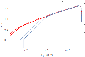
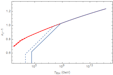
Figure 2: The maximum measurable spectral index $n_{I}-1$ as a function of $T_{RH}\in[100,5\times 10^{15}]$ GeV assuming an experimental sensitivity of $E_{k_{\rm max}}=10^{-3}$ corresponding to resolving $\Delta_{s}^{2}/\Delta_{\zeta}^{2}$ to $O(10^{-4}\%)$ at about $1$ Mpc length scale. The rest of the parameters are set at $\{k_{\rm max}/k_{\rm min}=10^{5};\,r_{b}=10^{-1},10^{-3};\,n_{\mathcal{O}}=5,6;\,S=(8\pi)^{-1},10^{-2}(8\pi)^{-1}\}$. (left) The bound on the tensor-to-scalar ratio $r$ has been taken to be $10^{-1}$. The lower solid curve for $T_{RH}\lesssim 10^{9}$ GeV corresponds to the reheating non-nonrenormalizable operator dimension of $n_{\mathcal{O}}=5$ just as in Fig. 1. The dotted curve corresponds to evaluation of fiducial spectral index at $k_{\rm max}$ instead of $k_{{\rm min}}$. As in Fig. 1, the correction is small because constraint 7 is not saturated even for $r_{b}=0.1$. As expected from increasing the experimental resolution by $10^{3}$, the maximum measurable spectral index has only gone up mildly to $n_{I}=2.25$ (from $n_{I}=2.12$). Note that unlike in Fig. 1, the bounds for $n_{\mathcal{O}}=6$ end at $T_{RH}=10^{2}$ GeV because we simply truncated the plot there (and not because $\omega_{\chi}>1$ there). The dashed curve corresponds to weakening the coefficient of the non-nonrenormalizable operator by a factor of 10 just as in Fig. 1. (right) Similar to the left plot except that $r_{b}$ has been set to $10^{-3}$.

Fig. 2 shows the case with $\{E_{k_{\rm max}}=10^{-3},\,k_{\rm max}/k_{\rm min}=10^{5};\,r_{b}=10^{-1},10^{-3};\,n_{\mathcal{O}}=5,6;\,S=(8\pi)^{-1},10^{-2}(8\pi)^{-1}\}$. Decreasing $E_{k_{\rm max}}$ to $10^{-3}$ means increasing the experimental sensitivity (i.e., $\Delta_{s}^{2}/\Delta_{\zeta}^{2}$ is resolved to $10^{-6}$ instead of order unity – an extremely optimistic view of the foreseeable future that is chosen to illustrate the insensitivity of the bound to experimental precision). This changes the measurable maximal spectral index logarithmically to about $n_{I}=2.25$ (from $n_{I}=2.1$ when $E_{k_{\rm max}}=1$). Hence, although increasing experimental sensitivity changes the measurable blue spectral index, the logarithmic nature of the increase makes these numbers experimentally meaningful for at least a many decades time scale. As before, the maximum temperature estimated in Eq. (48) agrees with the right end of the plot to better than 30% and the maximum $n_{I}-1$ agrees with Eq. (50) to better than 10%. For the $r_{b}=0.1$ plot (left plot), the reason why there is a drop of $n_{I}-1$ near $T_{RH}\sim 5\times 10^{15}$ GeV is the same reason as in the explanation for Fig. 1. Note that unlike in Fig. 1, the bounds for $n_{\mathcal{O}}=6$ end at $T_{RH}=10^{2}$ GeV because we simply truncated the plot there (and not because $\omega_{\chi}>1$ there).

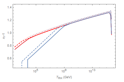
Figure 3: Similar to the left Fig. 2 except with $k_{\rm max}/k_{\rm min}=10^{7}$ (i.e. $k_{\rm max}$ is at the scale of 10 kpc). The bound on the maximum spectral index $n_{I}$ is only logarithmically sensitive to $k_{\rm max}/k_{\rm min}$ as it is now about 2.35 instead of 2.25. The features of the plots are explained as in previous figures. As before, the dotted curve corresponds to the evaluation of the spectral index with the fiducial $k$ value of $k_{\rm max}$ instead of $k_{\rm min}$.

Finally, to be extremely optimistic regarding short distance scale probes of cosmology, in Fig. 3 we consider the $n_{I}-1$ bound with an experimental probe length scale of $k_{\rm max}/k_{\rm min}=10^{7}$ (i.e. $k_{\rm max}$ is at the scale of 10 kpc) with the other parameters set at $\{E_{k_{\rm max}}=10^{-3},\,r_{b}=10^{-1},10^{-3};\,n_{\mathcal{O}}=5,6;\,S=(8\pi)^{-1},10^{-2}(8\pi)^{-1}\}$. The maximum spectral index increases as expected in a mild manner to $n_{I}=2.35$ (from $n_{I}=2.25$ with $k_{\rm max}/k_{\rm min}=10^{5}$). Note that this $k_{\rm max}/k_{\rm min}$ lies near the edge of constraint 11 in accordance with Eq. (60).

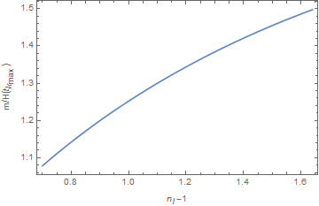
Figure 4: $m/H(t_{k_{\rm max}})$ is plotted as a function of $n_{I}-1$ defined according to Eq. (8) for the severest parametric choices of $r_{b}=0.1$ and $k_{\rm max}/k_{\rm min}=10^{7}$. This shows constraint 13 is satisfied for $n_{I}-1\lesssim 1.6$.

Also, constraint 13 can be shown to be generically satisfied in the $n_{I}-1$ and $k_{\rm max}/k_{\mbox{min }}$ region of our interest. For example, Fig. 4 shows $m/H(t_{k_{\rm max}})$ as a function of $n_{I}-1$ defined according to Eq. (8) for the parametric choices of $r_{b}=0.1$ and $k_{\rm max}/k_{{\rm min}}=10^{7}$ (which is the most constrained among the scenarios we are interested in). We see that since we have considered only $n_{I}-1\lesssim 1.6$, constraint 13 will be satisfied.

Note that for the numerical computations discussed thus far, only the background fields are evolved fully numerically to determine $\omega_{\chi}$ while analytic approximations relying on $H(t)$ being constant have been used to compute $\Delta_{s}^{2}/\omega_{\chi}^{2}$ in accordance with Chung:2015pga . For $r\ll 0.1$ we have $\epsilon_{k_{i}}\ll 1$, and $H(t)$ evolution does not present much of a correction. However, for $r_{b}=0.1$ in the plots above, there may be a worry that the numerical computation of $\Delta_{s}^{2}/\omega_{\chi}^{2}$ would deviate significantly from the approximations. One symptom of the analytic mode functions destroying the accuracy of $\Delta_{s}^{2}/\omega_{\chi}^{2}$ can be tested by comparing the answers for two different fiducial values of $k_{0}$.

The parametric spectral indices $n_{I}-1$ shown in Figs. 1 through 3 (except for the dotted curves) correspond to the $(k/k_{0}){}^{n_{I}-1}$ approximate parameterization with $k_{0}$ chosen at $k_{0}=k_{i}$ which is the longest observable wave vector. For $H_{i}$ corresponding to saturating constraint 7 with $r\lesssim 10^{-2}$, this is a good parameterization: i.e., in Figs. 1 through 3, plots with $r_{b}=10^{-3}$ can be taken to be accurate to better than 1%. However, if $H_{i}$ saturates the limit of constraint 7 with $r\approx 10^{-1}$, $H(t)$ would evolve nontrivially during inflation. In that case, there is a worry as to whether the $(k/k_{i})^{n_{I}-1}$ parameterization is inaccurate for the $r_{b}=0.1$ cases. For example, if we saturate constraint 7 with $r_{b}=10^{-1}$, a more accurate approximation of the observed spectrum near $k_{\rm max}$ should have the fiducial value $k_{0}=k_{\rm max}$ (at the expense of computing $\chi_{0}(t_{k_{0}})$ numerically). Fortunately, we find numerically that constraint 7 is never saturated even with $r_{b}=0.1$ because of the effects discussed in Eq. (73). The accuracy of the analytic spectrum calculation can also be seen in the dotted curves of Figs. 1 through 3 which were computed numerically.By explicit computation, we have checked that $n_{I}-1$ computed with mode function evolution evolved fully numerically matches the $n_{I}-1$ computed through the Bessel function with $k_{0}$ shifted to $k_{\rm max}$ (and $\chi_{0}(t_{k_{\rm max}})$ computed numerically) to better than a few percent.

Hence, we conclude from Fig. 4 that any measurement of $n_{I}>2.4$ for CDM-photon isocurvature perturbations in the foreseeable future indicates the responsible dynamical degree of freedom during inflation cannot be a constant mass linear spectator field.

V Models: What Happens With a Dynamical Mass?

In Chung:2015pga , it was shown that spectral indices as large as $n_{I}=3.8$ (but not $n_{I}=4$) can be achieved in the context of a dynamical VEV breaking the Peccei-Quinn (PQ) symmetry. This is of interest because $n_{I}=3$ is considered to be observable for example by the Square Kilometer Array Takeuchi:2013hza . Here, we discuss why a time-dependent mass during inflation can evade the bound discussed around Fig. 3. Suppose the mass of the field $\chi$ responsible for the linear spectator isocurvature makes a transition at time $t_{c}$ from value $m$ to zero. According to corollary 2 of Chung:2015pga , the modes $k<k_{c}$ that leave the horizon earlier than the time of the mass transition still have the form of Eq. (6), where if the slow-roll evolution is neglected, the critical wave vector is given by

$$k_{c}\sim k_{\rm min}\exp[N_{c}],$$ (77)

in which

$$N_{c}\equiv H_{i}(t_{c}-t_{k_{\rm min}})$$ (78)

is the number of efolds from the beginning of inflation. For $k_{c}\sim 10^{7}\,k_{\rm min}$, the number of efolds for which this occurs must be at least $N_{c}\sim 16$ efolds. All of these modes are governed by massive scalar field quantum fluctuations giving a blue spectrum. In addition, the background field $\chi_{0}(t)$ dilutes as

$$\chi_{0}(t)\propto\exp[-\frac{n_{I}-1}{2}N_{c}],$$ (79)

which dilutes the total isocurvature by an important factor:

$$\Delta_{s}^{2}\propto\exp[-2\left(n_{I}-1\right)N_{c},]$$ (80)

which is analogous to Eq. (35). The field theory up to this point behaves just as in the constant mass scenarios we have been discussing.

However, after the mass transition to masslessness completes, the background field $\chi_{0}(t)$ behaves as a constant massless field until the end of inflation. Hence, compared to the constant mass case, the isocurvature perturbations receive a boost of

$$\frac{\Delta_{s}^{2}(\mbox{time dependent mass})}{\Delta_{s}^{2}(\mbox{constant mass})}\propto\exp[2\left(n_{I}-1\right)(N_{e}-N_{c})]$$ (81)

in which $N_{e}$ is the total number of efolds as usual. Since $N_{e}\sim 50$, the enhancement for $N_{c}\sim 16$ scenario is enormous. This is the intuitive explanation with which time-dependent mass situations can evade the blue spectral index bounds for the time-independent mass situation that has been the main focus of this paper. One observational signature of the mass transition Kasuya:2009up is the existence of a flat isocurvature spectrum (for $k>k_{c}$) in addition to the blue spectrum ($k<k_{c}$). On the other hand, if there is a limited $k$-range accessible experimentally, it may not be easy to observe the break in the spectrum.

A natural question is then what class of models naturally produce these time dependent masses. Note that the crucial ingredient in being able to generate the large enhancement Eq. (81) is the transition from $m/H_{i}\sim O(1)$ to $m/H_{i}\ll 1$. If $H_{i}$ is the natural minimum energy scale for the masses of the scalar dynamical degrees of freedom (as is the case for example in supergravity models), then a symmetry needs to naturally lead to $m/H_{i}\ll 1$. Hence, one crucial ingredient for natural isocurvature models with $n_{I}$ larger than the bound presented for the constant mass case is a symmetry $X$ protecting the $\chi$ mass from Hubble scale corrections to its mass. A second ingredient is a temporary (but lasting many efolds) mass generation mechanism. This second ingredient is necessary to generate the blue spectrum.

In the supersymmetric axion scenario of Kasuya:2009up , the symmetry $X$ is the Peccei-Quinn (PQ) symmetry non-linearly realized as a shift symmetry of the axion field. The PQ symmetry breaking fields $\Phi_{\pm}$ are displaced from the minimum of the effective potential during inflation (in a way in which PQ symmetry is always broken) such that the coset symmetry $X$ is actually broken by $\partial_{t}\Phi_{\pm}$ through the kinetic structure of the axion: i.e., the Nambu-Goldstone theorem does not apply because the system is not in vacuum. As $\Phi_{\pm}$ fields roll toward the vacuum (where the PQ breaking persists), the axions behave as a massive field with mass of the order of $H_{i}$ due to the supergravity structure of the Kähler potential. After $\Phi_{\pm}$ reaches the vacuum and the kinetic energy dilutes to the point of $\partial_{t}\Phi_{\pm}\ll H_{i}\Phi_{\pm}$, $X$ is restored axions become massless, up to the small explicit PQ breaking contribution.

Although it is possible to tune parameters and initial conditions to obtain almost flat potentials, the Nambu-Goldstone models with out-of-equilibrium symmetry-breaking time-dependent VEVs seem to be the simplest natural model. From this perspective, any experiment measuring a CDM-photon isocurvature perturbations with $n_{I}\gtrsim 2.4$ may be finding evidence for a dynamical degree of freedom during inflation that has a coset shift symmetry.

VI Conclusions

We have considered a constant mass spectator linear isocurvature degree of freedom during inflation and answered the question of what is the largest measurable blue spectral index that can be produced via such a mechanism. We have shown that the largest measurable spectral index is less than 2.4 in the foreseeable future with only logarithmic sensitivity to experimental precision characterized by $\{E_{k_{\rm max}},\,k_{\rm max}/k_{\rm min}\}$ and experimental constraints such as the tensor-to-scalar ratio $r_{b}$. This means that any future measurements of the isocurvature spectral index above this bound would give weight to the hypothesis that there is a spectator field with a time-dependent mass during inflation.

We have also considered how for reheating temperatures much smaller than the maximum allowed by tensor perturbation bound, the maximum observable spectral index decreases. This would be relevant if there were specific inflationary models under consideration with a fixed reheating scenario or model-dependent phenomenological bounds on the reheating temperature such as those that arise from cosmologically dangerous gravitinos. For part of this smaller reheating temperature dependent bound, we have used the assumption that there is at least a gravitationally suppressed non-nonrenormalizable operator of dimension 5 or 6 that can contribute to reheating. This assumption sets a bound on the maximum separation between the reheating temperature and the expansion rate at the end of inflation in certain cases.

One has to keep in mind that the maximum derived in this paper has some obvious caveats. First, since we have only considered linear spectator scenarios, we have not examined what the maximum blue spectral index would be if we allowed $\delta\chi$ to be of order $\chi_{0}$ . Since we have imposed $\chi_{0}>H/(2\pi)$ and $\delta\chi$ is at most of order $H/(2\pi)$, one might think that the current estimate will stand even after including the $\delta\chi\gtrsim\chi_{0}$ scenarios. On the other hand, the $n_{I}-1$ of quadratic isocurvature scenarios (i.e. scenarios in which the isocurvature perturbations are proportional to $\Delta_{s}^{2}\propto\langle\delta\chi^{2}\delta\chi^{2}\rangle$) is twice that of the linear spectator scenario Chung:2011xd ; Chung:2004nh ; Liddle:1999pr . However, a preliminary investigation shows that this factor of 2 in the power only gives an enhancement of the form

$$\max[n_{I}-1]\propto\frac{1-\frac{1}{2N_{e}}\ln[k_{\rm max}/k_{{\rm min}}]}{1-\frac{1}{N_{e}}\ln[k_{\rm max}/k_{{\rm min}}]}$$ (82)

multiplying a difficult to compute suppression (originating from the quantum nature of the particle production in contrast with the classical VEV displacements of the linear spectator scenario), resulting in a similar maximum spectral bound at best. However, given that the dependence of the relic density and the spectral amplitude with $n_{I}-1$ is somewhat complicated due to their dependence on the long time mode evolution Chung:2011xd , it would be worthwhile confirming the quadratic isocurvature estimate more carefully.

Another caveat is that we have assumed a “standard” slow-roll, effectively single-field inflationary scenario with only one reheating period. Most non-minimal extensions will dilute the VEV energy density leading to a smaller upper bound. In that sense, most of the non-minimal extensions are not likely to change this general picture. Even in the situation in which $\chi_{0}$ makes a phase transition after inflation (e.g. $\chi_{0}$ goes from $v_{1}$ to $v_{2}$) such that $\omega_{\chi}$ (now proportional to $v_{2}^{2}$) is generated after inflation (thereby evading the inflationary dilution), since it is really $\delta\chi$ that is diluting during inflation (even though we have been rewriting it as $\omega_{\chi}\delta\chi/|\chi_{0}-v_{1}|$ being constant during inflation), this does not help us to evade the bound.

Finally, we have assumed a sampling of inflationary space characterized by $\{\epsilon_{i},H_{i},t_{e}\}$, while there are infinitely more ways to tune the inflationary models. On the other hand, even the addition of $\epsilon_{i}$ (versus a non-evolving scenario of $H(t)$ during inflation) produced only about a 10% change in $n_{I}-1$. Hence, we believe this limitation of sampling is not severely restrictive.

It is indeed intriguing that future cosmological inhomogeneity measurements of $n_{I}\gtrsim 2.4$ may uncover the following new features of dark matter: (i) dark matter had to have a time dependence in its mass in its evolution history in the context of an inflationary universe, and (ii) dark matter mass was of order of the expansion rate during inflation. From our current model building tool-kit, arguably the most appealing picture that would emerge is that the dark matter is a field possessing a fundamental shift symmetry just like the axion.

Appendix A Background Solution

For this section, we set the time at which the observable longest wavelength mode leaves the horizon to be time $t_{k_{i}}=0$. We can model a very large class of slow-roll inflationary models with the Hubble expansion rate function parameterized (with three constants $\{\epsilon_{k_{i}},H_{i},t_{e}\}$, where $t_{e}$ approximately replaces $\eta_{V}$ in the usual slow-roll parameterization scheme) as

$$H\approx\left\{\begin{array}[]{ccc}H_{i}(1-\epsilon_{k_{i}}H_{i}t)&&0<t<t_{e}\\ \frac{H_{i}(1-\epsilon_{k_{i}}H_{i}t_{e})}{1+\frac{3}{2}(t-t_{e})H_{i}(1-H_{i}\epsilon_{k_{i}}t_{e})}&&t_{e}<t<t_{RH}\end{array}\right\},$$ (83)

in which $\Delta t\equiv t-t_{i}$ and $t_{RH}$ is the time of reheating. This ansatz accurately (at the order of 10% level) both quadratic inflation and hybrid inflation. Note also that as long as the number of efolds is fewer than

$$N_{max}\equiv\frac{1}{2\epsilon_{k_{i}}}\approx\frac{4\pi^{2}M_{p}^{2}\Delta_{\zeta}^{2}(k_{i})}{H_{i}^{2}},$$ (84)

the quantity $H$ will never go negative.

After the end of inflation, the solution of the field evolution equation

$$\ddot{\chi}_{0}(t)+3H\dot{\chi}_{0}(t)+m_{\chi}^{2}\chi_{0}(t)=0$$ (85)

takes the simple form

$$\chi_{0}(t)=\frac{e_{1}\cos(m_{\chi}\Delta t)+e_{2}\sin(m\Delta t)}{1-\frac{3}{2}H_{i}\Delta t(\epsilon_{k_{i}}H_{i}t_{e}-1)}$$ (86)

where $\Delta t=t-t_{e}$.

We could in principle solve the equation of motion (Eq. (85)) exactly in this class of models in terms of hypergeometric functions and Hermite polynomials

$$\chi_{0}=C_{1}\,H_{\frac{m^{2}}{3\epsilon_{k_{i}}H_{i}^{2}}}\left(-\sqrt{\frac{3}{2\epsilon_{k_{i}}}}+\sqrt{\frac{3}{2}\epsilon_{k_{i}}}H_{i}t\right)+C_{2}\,{}_{1}F_{1}\left(\frac{-m^{2}}{6\epsilon_{k_{i}}H_{i}^{2}};\frac{1}{2};\left(\sqrt{\frac{3}{2\epsilon_{k_{i}}}}-\sqrt{\frac{3}{2}\epsilon_{k_{i}}}H_{i}t\right)^{2}\right).$$ (87)

However, because $\epsilon_{k_{i}}$ is small, these special functions must be evaluated in exponentially large and small numerical regions and added together. Such a route seems numerically unstable, in addition to being opaque. In practice, it is easier to handle numerically the solution to the equation of motion subject to the boundary condition

$$\dot{\chi}_{0}(0)=-\left(\frac{3}{2}-\nu_{i}\right)H_{i}\chi_{0}(0),$$ (88)

which embodies the assumptions that the spectral index is of order unity and the field is rolling in a slow-roll fashion, initially.

We can match the solution before and after the end of inflation to write the solution after the end of inflation as

$$\chi_{0}(t)=K_{1}\left[\frac{H(t)}{H(t_{e})}\right]\cos(m\Delta t+K_{2})$$ (89)

$$K_{1}\equiv\sqrt{\mathcal{A}}\chi_{0}(0)\exp\left[-\frac{1}{2}(3-2\nu_{k_{i}})H_{i}t_{e}\right],$$ (90)

in which $K_{2}$ is a phase. The amplitude is given by

$$\sqrt{\mathcal{A}}=\frac{\chi_{0}(t_{e})e^{\frac{1}{2}(3-2\nu_{i})H_{i}t_{e}}}{\chi_{0}(0)}\sqrt{1+\frac{\left[1-\epsilon_{k_{i}}H_{i}t_{e}+\frac{2}{3}\dot{\chi}_{0}(t_{e})/\left(H_{i}\chi_{0}(t_{e})\right)\right]^{2}}{1-\frac{4}{9}\nu_{i}^{2}}},$$ (91)

in which we note that $\chi_{0}(t_{e})\exp\left[\frac{1}{2}(3-2\nu_{i})H_{i}t_{e}\right]$ is the initial value $\chi_{0}(0)$ for $\epsilon_{k_{i}}=0$. Hence, it is more convenient numerically to solve for $\chi_{0}(t)\exp\left[\frac{1}{2}(3-2\nu_{i})H_{i}t\right]$ than $\chi_{0}(t)$. The exponential suppression of $\chi_{0}(t_{e})\exp\left[\frac{1}{2}(3-2\nu_{i})H_{i}t_{e}\right]/\chi_{0}(0)$ still occurs when $9-4m^{2}/H_{i}^{2}/(1-\epsilon_{k_{i}}H_{i}t_{e})^{2}<0$. In this notation, the dark matter fraction $\omega_{\chi}$ is

$$\omega_{\chi}=\frac{K_{1}^{2}}{M_{p}^{2}}\frac{m^{2}}{H^{2}(t_{e})}\frac{T_{RH}}{T_{eq}}R.$$ (92)

where $R$ is defined in Eq. 25.

References

- (1) A. A. Starobinsky, A New Type of Isotropic Cosmological Models Without Singularity, Phys.Lett. B91 (1980) 99–102.
- (2) K. Sato, First Order Phase Transition of a Vacuum and Expansion of the Universe, Mon.Not.Roy.Astron.Soc. 195 (1981) 467–479.
- (3) A. D. Linde, A New Inflationary Universe Scenario: A Possible Solution of the Horizon, Flatness, Homogeneity, Isotropy and Primordial Monopole Problems, Phys.Lett. B108 (1982) 389–393.
- (4) V. F. Mukhanov and G. Chibisov, Quantum Fluctuation and Nonsingular Universe. (In Russian), JETP Lett. 33 (1981) 532–535.
- (5) A. Albrecht and P. J. Steinhardt, Cosmology for Grand Unified Theories with Radiatively Induced Symmetry Breaking, Phys.Rev.Lett. 48 (1982) 1220–1223.
- (6) S. Hawking and I. Moss, FLUCTUATIONS IN THE INFLATIONARY UNIVERSE, Nucl.Phys. B224 (1983) 180.
- (7) A. H. Guth and S. Pi, Fluctuations in the New Inflationary Universe, Phys.Rev.Lett. 49 (1982) 1110–1113.
- (8) A. A. Starobinsky, Dynamics of Phase Transition in the New Inflationary Universe Scenario and Generation of Perturbations, Phys.Lett. B117 (1982) 175–178.
- (9) J. M. Bardeen, P. J. Steinhardt, and M. S. Turner, Spontaneous Creation of Almost Scale - Free Density Perturbations in an Inflationary Universe, Phys.Rev. D28 (1983) 679.
- (10) K. Freese, J. A. Frieman, and A. V. Olinto, Natural inflation with pseudo - Nambu-Goldstone bosons, Phys. Rev. Lett. 65 (1990) 3233–3236.
- (11) Planck Collaboration, P. A. R. Ade et. al., Planck 2015 results. XIII. Cosmological parameters, arXiv:1502.0158.
- (12) Planck Collaboration, P. A. R. Ade et. al., Planck 2015 results. XX. Constraints on inflation, arXiv:1502.0211.
- (13) Planck Collaboration Collaboration, P. Ade et. al., Planck 2013 results. I. Overview of products and scientific results, Astron.Astrophys. 571 (2014) A1, [arXiv:1303.5062].
- (14) Planck Collaboration Collaboration, P. Ade et. al., Planck 2013 results. XVI. Cosmological parameters, Astron.Astrophys. 571 (2014) A16, [arXiv:1303.5076].
- (15) Planck Collaboration Collaboration, P. Ade et. al., Planck 2013 results. XXII. Constraints on inflation, Astron.Astrophys. 571 (2014) A22, [arXiv:1303.5082].
- (16) Planck Collaboration Collaboration, P. Ade et. al., Planck 2013 results. XXIII. Isotropy and statistics of the CMB, Astron.Astrophys. 571 (2014) A23, [arXiv:1303.5083].
- (17) Planck Collaboration Collaboration, P. Ade et. al., Planck 2013 Results. XXIV. Constraints on primordial non-Gaussianity, Astron.Astrophys. 571 (2014) A24, [arXiv:1303.5084].
- (18) SPT Collaboration, R. Keisler et. al., Measurements of Sub-degree B-mode Polarization in the Cosmic Microwave Background from 100 Square Degrees of SPTpol Data, Astrophys. J. 807 (2015), no. 2 151, [arXiv:1503.0231].
- (19) G. Hinshaw, D. Larson, E. Komatsu, D. Spergel, C. Bennett, et. al., Nine-Year Wilkinson Microwave Anisotropy Probe (WMAP) Observations: Cosmological Parameter Results, arXiv:1212.5226.
- (20) WMAP Collaboration Collaboration, E. Komatsu et. al., Seven-Year Wilkinson Microwave Anisotropy Probe (WMAP) Observations: Cosmological Interpretation, Astrophys.J.Suppl. 192 (2011) 18, [arXiv:1001.4538].
- (21) QUaD collaboration Collaboration, . M. Brown et. al., Improved measurements of the temperature and polarization of the CMB from QUaD, Astrophys.J. 705 (2009) 978–999, [arXiv:0906.1003].
- (22) C. Reichardt, P. Ade, J. Bock, J. R. Bond, J. Brevik, et. al., High resolution CMB power spectrum from the complete ACBAR data set, Astrophys.J. 694 (2009) 1200–1219, [arXiv:0801.1491].
- (23) ACT Collaboration Collaboration, J. Fowler et. al., The Atacama Cosmology Telescope: A Measurement of the 600 ell 8000 Cosmic Microwave Background Power Spectrum at 148 GHz, Astrophys.J. 722 (2010) 1148–1161, [arXiv:1001.2934].
- (24) M. Lueker, C. Reichardt, K. Schaffer, O. Zahn, P. Ade, et. al., Measurements of Secondary Cosmic Microwave Background Anisotropies with the South Pole Telescope, Astrophys.J. 719 (2010) 1045–1066, [arXiv:0912.4317].
- (25) C. Hikage, M. Kawasaki, T. Sekiguchi, and T. Takahashi, CMB constraint on non-Gaussianity in isocurvature perturbations, JCAP 1307 (2013) 007, [arXiv:1211.1095].
- (26) A. J. Ross et. al., The Clustering of Galaxies in SDSS-III DR9 Baryon Oscillation Spectroscopic Survey: Constraints on Primordial Non-Gaussianity, Mon. Not. Roy. Astron. Soc. 428 (2013) 1116–1127, [arXiv:1208.1491].
- (27) W. J. Percival, S. Cole, D. J. Eisenstein, R. C. Nichol, J. A. Peacock, et. al., Measuring the Baryon Acoustic Oscillation scale using the SDSS and 2dFGRS, Mon.Not.Roy.Astron.Soc. 381 (2007) 1053–1066, [arXiv:0705.3323].
- (28) SDSS Collaboration Collaboration, D. J. Eisenstein et. al., Detection of the baryon acoustic peak in the large-scale correlation function of SDSS luminous red galaxies, Astrophys.J. 633 (2005) 560–574, [astro-ph/0501171].
- (29) J. Preskill, M. B. Wise, and F. Wilczek, Cosmology of the Invisible Axion, Phys.Lett. B120 (1983) 127–132.
- (30) L. Abbott and P. Sikivie, A Cosmological Bound on the Invisible Axion, Phys.Lett. B120 (1983) 133–136.
- (31) M. Dine and W. Fischler, The Not So Harmless Axion, Phys.Lett. B120 (1983) 137–141.
- (32) M. Axenides, R. H. Brandenberger, and M. S. Turner, Development of Axion Perturbations in an Axion Dominated Universe, Phys.Lett. B126 (1983) 178.
- (33) P. J. Steinhardt and M. S. Turner, Saving the Invisible Axion, Phys.Lett. B129 (1983) 51.
- (34) M. S. Turner, F. Wilczek, and A. Zee, Formation of Structure in an Axion Dominated Universe, Phys.Lett. B125 (1983) 35.
- (35) A. D. Linde, GENERATION OF ISOTHERMAL DENSITY PERTURBATIONS IN THE INFLATIONARY UNIVERSE, JETP Lett. 40 (1984) 1333–1336.
- (36) M. S. Turner, Cosmic and Local Mass Density of Invisible Axions, Phys.Rev. D33 (1986) 889–896.
- (37) D. Seckel and M. S. Turner, Isothermal Density Perturbations in an Axion Dominated Inflationary Universe, Phys.Rev. D32 (1985) 3178.
- (38) E. W. Kolb and M. S. Turner, The Early universe, Front.Phys. 69 (1990) 1–547.
- (39) D. Polarski and A. A. Starobinsky, Isocurvature perturbations in multiple inflationary models, Phys.Rev. D50 (1994) 6123–6129, [astro-ph/9404061].
- (40) C. Gordon, D. Wands, B. A. Bassett, and R. Maartens, Adiabatic and entropy perturbations from inflation, Phys.Rev. D63 (2001) 023506, [astro-ph/0009131].
- (41) P. Fox, A. Pierce, and S. D. Thomas, Probing a QCD string axion with precision cosmological measurements, hep-th/0409059.
- (42) P. Sikivie, Axion Cosmology, Lect.Notes Phys. 741 (2008) 19–50, [astro-ph/0610440].
- (43) M. Beltran, J. Garcia-Bellido, and J. Lesgourgues, Isocurvature bounds on axions revisited, Phys.Rev. D75 (2007) 103507, [hep-ph/0606107].
- (44) M. P. Hertzberg, M. Tegmark, and F. Wilczek, Axion Cosmology and the Energy Scale of Inflation, Phys.Rev. D78 (2008) 083507, [arXiv:0807.1726].
- (45) K. A. Malik and D. Wands, Cosmological perturbations, Phys.Rept. 475 (2009) 1–51, [arXiv:0809.4944].
- (46) D. Langlois and A. Lepidi, General treatment of isocurvature perturbations and non-Gaussianities, JCAP 1101 (2011) 008, [arXiv:1007.5498].
- (47) L. Visinelli and P. Gondolo, Axion cold dark matter in view of BICEP2 results, Phys.Rev.Lett. 113 (2014) 011802, [arXiv:1403.4594].
- (48) K. Choi, K. S. Jeong, and M.-S. Seo, String theoretic QCD axions in the light of PLANCK and BICEP2, JHEP 1407 (2014) 092, [arXiv:1404.3880].
- (49) M. Kawasaki, N. Kitajima, and F. Takahashi, Relaxing Isocurvature Bounds on String Axion Dark Matter, Phys. Lett. B737 (2014) 178–184, [arXiv:1406.0660].
- (50) K. Harigaya, M. Ibe, M. Kawasaki, and T. T. Yanagida, Dynamics of Peccei-Quinn Breaking Field after Inflation and Axion Isocurvature Perturbations, arXiv:1507.0011.
- (51) K. Kadota, T. Kobayashi, and H. Otsuka, Axion inflation with cross-correlated axion isocurvature perturbations, arXiv:1509.0452.
- (52) R. Peccei and H. R. Quinn, CP Conservation in the Presence of Instantons, Phys.Rev.Lett. 38 (1977) 1440–1443.
- (53) S. Weinberg, A New Light Boson?, Phys.Rev.Lett. 40 (1978) 223–226.
- (54) F. Wilczek, Problem of Strong p and t Invariance in the Presence of Instantons, Phys.Rev.Lett. 40 (1978) 279–282.
- (55) D. J. Chung, E. W. Kolb, and A. Riotto, Superheavy dark matter, Phys.Rev. D59 (1999) 023501, [hep-ph/9802238]. In *Venice 1999, Neutrino telescopes, vol. 2* 217-237.
- (56) D. J. Chung, E. W. Kolb, and A. Riotto, Nonthermal supermassive dark matter, Phys.Rev.Lett. 81 (1998) 4048–4051, [hep-ph/9805473].
- (57) V. A. Kuzmin and I. I. Tkachev, Ultrahigh-energy cosmic rays and inflation relics, Phys.Rept. 320 (1999) 199–221, [hep-ph/9903542].
- (58) V. Kuzmin and I. Tkachev, Matter creation via vacuum fluctuations in the early universe and observed ultrahigh-energy cosmic ray events, Phys.Rev. D59 (1999) 123006, [hep-ph/9809547].
- (59) D. J. Chung, P. Crotty, E. W. Kolb, and A. Riotto, On the gravitational production of superheavy dark matter, Phys.Rev. D64 (2001) 043503, [hep-ph/0104100].
- (60) D. J. Chung, Classical inflation field induced creation of superheavy dark matter, Phys.Rev. D67 (2003) 083514, [hep-ph/9809489].
- (61) R. Aloisio, S. Matarrese, and A. V. Olinto, Super Heavy Dark Matter in light of BICEP2, Planck and Ultra High Energy Cosmic Rays Observations, JCAP 08 (2015) 024, [arXiv:1504.0131].
- (62) M. A. Fedderke, E. W. Kolb, and M. Wyman, Irruption of massive particle species during inflation, Phys. Rev. D91 (2015), no. 6 063505, [arXiv:1409.1584].
- (63) D. J. H. Chung, H. Yoo, and P. Zhou, Fermionic Isocurvature Perturbations, arXiv:1306.1966.
- (64) D. J. H. Chung, H. Yoo, and P. Zhou, Quadratic Isocurvature Cross-Correlation, Ward Identity, and Dark Matter, Phys.Rev. D87 (2013), no. 12 123502, [arXiv:1303.6024].
- (65) WMAP Collaboration Collaboration, E. Komatsu et. al., Seven-Year Wilkinson Microwave Anisotropy Probe (WMAP) Observations: Cosmological Interpretation, Astrophys.J.Suppl. 192 (2011) 18, [arXiv:1001.4538].
- (66) J. Väliviita and T. Giannantonio, Constraints on primordial isocurvature perturbations and spatial curvature by Bayesian model selection, Physical Review D 80 (Dec., 2009).
- (67) I. Sollom, A. Challinor, and M. P. Hobson, Cold Dark Matter Isocurvature Perturbations: Constraints and Model Selection, Phys.Rev. D79 (2009) 123521, [arXiv:0903.5257].
- (68) WMAP Collaboration Collaboration, E. Komatsu et. al., Five-Year Wilkinson Microwave Anisotropy Probe (WMAP) Observations: Cosmological Interpretation, Astrophys.J.Suppl. 180 (2009) 330–376, [arXiv:0803.0547].
- (69) R. Bean, J. Dunkley, and E. Pierpaoli, Constraining Isocurvature Initial Conditions with WMAP 3-year data, Phys.Rev. D74 (2006) 063503, [astro-ph/0606685].
- (70) P. Crotty, J. Garcia-Bellido, J. Lesgourgues, and A. Riazuelo, Bounds on isocurvature perturbations from cosmic microwave background and large scale structure data, Physical Review Letters 91 (2003), no. 17 171301.
- (71) C. Hikage, K. Koyama, T. Matsubara, T. Takahashi, and M. Yamaguchi, Limits on Isocurvature Perturbations from Non-Gaussianity in WMAP Temperature Anisotropy, Mon.Not.Roy.Astron.Soc. 398 (2009) 2188–2198, [arXiv:0812.3500]. * Brief entry *.
- (72) Y. Takeuchi and S. Chongchitnan, Constraining isocurvature perturbations with the 21cm emission from minihaloes, arXiv:1311.2585.
- (73) D. J. H. Chung and H. Yoo, Elementary Theorems Regarding Blue Isocurvature Perturbations, Phys. Rev. D91 (2015), no. 8 083530, [arXiv:1501.0561].
- (74) S. Kasuya and M. Kawasaki, Axion isocurvature fluctuations with extremely blue spectrum, Phys.Rev. D80 (2009) 023516, [arXiv:0904.3800].
- (75) J. B. Dent, D. A. Easson, and H. Tashiro, Cosmological constraints from CMB distortion, Phys.Rev. D86 (2012) 023514, [arXiv:1202.6066].
- (76) J. Chluba and D. Grin, CMB spectral distortions from small-scale isocurvature fluctuations, Mon.Not.Roy.Astron.Soc. 434 (2013) 1619–1635, [arXiv:1304.4596].
- (77) T. Sekiguchi, H. Tashiro, J. Silk, and N. Sugiyama, Cosmological signatures of tilted isocurvature perturbations: reionization and 21cm fluctuations, JCAP 1403 (2014) 001, [arXiv:1311.3294].
- (78) N. Arkani-Hamed and J. Maldacena, Cosmological Collider Physics, arXiv:1503.0804.
- (79) X. Chen and Y. Wang, Quasi-Single Field Inflation with Large Mass, JCAP 1209 (2012) 021, [arXiv:1205.0160].
- (80) N. Craig and D. Green, Testing Split Supersymmetry with Inflation, JHEP 07 (2014) 102, [arXiv:1403.7193].
- (81) E. Dimastrogiovanni, M. Fasiello, and M. Kamionkowski, Imprints of Massive Primordial Fields on Large-Scale Structure, arXiv:1504.0599.
- (82) J. E. Lidsey, A. R. Liddle, E. W. Kolb, E. J. Copeland, T. Barreiro, and M. Abney, Reconstructing the inflation potential : An overview, Rev. Mod. Phys. 69 (1997) 373–410, [astro-ph/9508078].
- (83) W. H. Kinney, Inflation: Flow, fixed points and observables to arbitrary order in slow roll, Phys. Rev. D66 (2002) 083508, [astro-ph/0206032].
- (84) W. H. Kinney, E. W. Kolb, A. Melchiorri, and A. Riotto, WMAPping inflationary physics, Phys. Rev. D69 (2004) 103516, [hep-ph/0305130].
- (85) D. J. H. Chung and A. Enea Romano, Approximate consistency condition from running spectral index in slow-roll inflationary models, Phys. Rev. D73 (2006) 103510, [astro-ph/0508411].
- (86) N. Agarwal and R. Bean, Cosmological constraints on general, single field inflation, Phys. Rev. D79 (2009) 023503, [arXiv:0809.2798].
- (87) B. A. Powell, K. Tzirakis, and W. H. Kinney, Tensors, non-Gaussianities, and the future of potential reconstruction, JCAP 0904 (2009) 019, [arXiv:0812.1797].
- (88) R. Blumenhagen and E. Plauschinn, Towards Universal Axion Inflation and Reheating in String Theory, Phys. Lett. B736 (2014) 482–487, [arXiv:1404.3542].
- (89) M. Cicoli, G. Tasinato, I. Zavala, C. P. Burgess, and F. Quevedo, Modulated Reheating and Large Non-Gaussianity in String Cosmology, JCAP 1205 (2012) 039, [arXiv:1202.4580].
- (90) M. Cicoli and A. Mazumdar, Reheating for Closed String Inflation, JCAP 1009 (2010), no. 09 025, [arXiv:1005.5076].
- (91) D. R. Green, Reheating Closed String Inflation, Phys. Rev. D76 (2007) 103504, [arXiv:0707.3832].
- (92) X. Chen and S. H. H. Tye, Heating in brane inflation and hidden dark matter, JCAP 0606 (2006) 011, [hep-th/0602136].
- (93) D. Chialva, G. Shiu, and B. Underwood, Warped reheating in multi-throat brane inflation, JHEP 01 (2006) 014, [hep-th/0508229].
- (94) A. R. Frey, A. Mazumdar, and R. C. Myers, Stringy effects during inflation and reheating, Phys. Rev. D73 (2006) 026003, [hep-th/0508139].
- (95) L. Kofman and P. Yi, Reheating the universe after string theory inflation, Phys. Rev. D72 (2005) 106001, [hep-th/0507257].
- (96) N. Arkani-Hamed, L. Motl, A. Nicolis, and C. Vafa, The String landscape, black holes and gravity as the weakest force, JHEP 06 (2007) 060, [hep-th/0601001].
- (97) J. Brown, W. Cottrell, G. Shiu, and P. Soler, Fencing in the Swampland: Quantum Gravity Constraints on Large Field Inflation, arXiv:1503.0478.
- (98) T. Rudelius, Constraints on Axion Inflation from the Weak Gravity Conjecture, JCAP 09 (2015) 020, [arXiv:1503.0079].
- (99) C. Cheung and G. N. Remmen, Naturalness and the Weak Gravity Conjecture, Phys. Rev. Lett. 113 (2014) 051601, [arXiv:1402.2287].
- (100) D. J. Chung and H. Yoo, Isocurvature Perturbations and Non-Gaussianity of Gravitationally Produced Nonthermal Dark Matter, Phys.Rev. D87 (2013) 023516, [arXiv:1110.5931].
- (101) D. J. Chung, E. W. Kolb, A. Riotto, and L. Senatore, Isocurvature constraints on gravitationally produced superheavy dark matter, Phys.Rev. D72 (2005) 023511, [astro-ph/0411468].
- (102) A. R. Liddle and A. Mazumdar, Perturbation amplitude in isocurvature inflation scenarios, Phys. Rev. D61 (2000) 123507, [astro-ph/9912349].