Outflow-Confined H II Regions. I. First Signposts of Massive Star Formation

Abstract

We present an evolutionary sequence of models of the photoionized disk-wind outflow around forming massive stars based on the Core Accretion model. The outflow is expected to be the first structure to be ionized by the protostar and can confine the expansion of the H II region, especially in lateral directions in the plane of the accretion disk. The ionizing luminosity increases as Kelvin-Helmholz contraction proceeds, and the H II region is formed when the stellar mass reaches $\sim 10\>$ – $\>20M_{\odot}$ depending on the initial cloud core properties. Although some part of outer disk surface remains neutral due to shielding by the inner disk and the disk wind, almost the whole of the outflow is ionized in $10^{3}$–$10^{4}{\rm yr}$ after initial H II region formation. Having calculated the extent and temperature structure of the H II region within the immediate protostellar environment, we then make predictions for the strength of its free-free continuum and recombination line emission. The free-free radio emission from the ionized outflow has a flux density of $\sim(20\>$–$\>200)\times(\nu/10{\rm GHz})^{p}\>{\rm mJy}$ for a source at a distance of 1 kpc with a spectral index $p\simeq 0.4\>$–$\>0.7$, and the apparent size is typically $\sim$500 AU at 10 GHz. The $\rm H40\alpha$ line profile has a width of about $100\>{\rm\>km\>s^{-1}}$. These properties of our model are consistent with observed radio winds and jets around forming massive protostars.

1. Introduction

The formation mechanism of massive stars remains much debated with Core Accretion, Competitive Accretion and even Protostellar Collisions still discussed (see Tan et al., 2014, for a recent review).

One of the key differences between high and low-mass protostars is that the former are expected to complete the later stages of their accretion while fusing hydrogen on the main sequence. Their photospheres should be hot and strong sources of Lyman continnum photons with energies $>13.6$ eV, which can photoionize H to create an H II region. These protostellar H II regions are important for at least two main reasons. First, by their long wavelength radio free-free and Hydrogen recombination line (HRL) emission they provide diagnostics of the massive star formation process. Second, the ionized gas reaches temperatures of $\sim 10^{4}$ K and its thermal pressure could be an important feedback process that regulates massive star formation, either by disrupting the wider scale accretion reservoir (i.e., core envelope or Bondi-Hoyle competitive accretion region: e.g., Dale et al., 2005; Peters et al., 2010, 2011) or by photoevaporation of the accretion disk (Hollenbach et al., 1994; Yorke & Welz, 1996; Richling & Yorke, 1997; McKee & Tan, 2008; Tanaka et al., 2013).

Our goal in this study is to present model calculations of the structure of the earliest-stage protostellar H II regions in the context of the Turbulent Core Model of McKee & Tan (2003) (hereafter, MT03). Early work in this direction was carried out by Tan & McKee (2003), who described these structures as “Outflow-Confined” H II regions, since the magneto-centrifugally-launched protostellar outflow (either disk-wind, X-wind or both) will be the first barrier to the ionizing photons.

Keto (2007) studied the structure and evolution of H II regions that are confined by the infalling flow onto the protostellar disk. However, their model did not include the effect of the MHD-driven outflow. If massive stars form in a scaled-up, but similar manner to low-mass stars, then we expect such outflows to always be present around massive protostars during their main accretion phase. Indeed, larger-scale collimated outflows are often observed to be driven from massive protostars (e.g., Beuther et al., 2002; Garay et al., 2007; López-Sepulcre et al., 2009)

A series of massive protostellar evolution calculations to predict continuum radiative transfer, especially infrared to sub-mm morphologies and spectral energy distributions (SEDs), has been carried out by Zhang & Tan (2011), Zhang et al. (2013), and Zhang et al. (2014) (hereafter, ZTH14). Here we will calculate the ionization structure and associated radio emission predicted by these protostellar evolutionary sequences.

Study of radio emission from massive protostars has a long history (see, e.g., Wood & Churchwell, 1989; Hoare et al., 2007; Tan et al., 2014). Ultra-compact ($\leq 0.1\>{\rm pc}$) and, especially, hyper-compact ($\leq 0.01\>{\rm pc}$) H II regions may include sources that are in the protostellar phase. Elongated radio continuum sources, e.g., radio “jets”, have been seen in a number of sources (e.g., Guzmán et al., 2012). The eventual goal of our work will be to compare the developed models with such observations, however, detailed comparison with individual sources, requiring tailored protostellar models, is deferred to future works in this series.

This paper is organized as follows. In §2 we describe our methods: in particular, we briefly review the protostellar evolution models, describe calculation of the photoionized structure and the radiative transfer of free-free continuum and HRL emission. Next, in §3, we present our results: especially, we explore the evolution of the photoionized regions for various initial core conditions and predict their observational features. In §4 we discuss the implications of our results, especially summarizing the evolution of the outflow confined H II regions, and making an initial comparison of our models with the general characteristics of observed HC/UC H II regions and radio winds/jets. We conclude in §5.

2. Methods

2.1. Evolution of protostars, disks, envelopes and outflows

Table 1Model lists

Models	$M_{\rm c}\>(M_{\odot})$	$\Sigma_{\rm cl}\>({\rm g~{}cm^{-2}})$	$m_{*}\>(M_{\odot})$	$r_{*}\>(R_{\odot})$	$T_{\rm*,acc}\>({\rm\times 10^{4}K})$	$L_{\rm*,acc}\>(\times 10^{4}L_{\odot})$	$\log_{10}S_{*,\rm acc}\>({\rm~{}s^{-1}})$
A12	60	1	12	12.9	2.33	4.4	46.5
A16			16	6.4	3.67	6.6	48.3
A24			24	6.4	3.90	8.5	48.6
Al08	60	0.316	8	14.0	1.59	1.1	43.9
Al12			12	4.7	3.27	2.3	47.5
Al16			16	5.1	3.43	3.2	47.8
Ah12	60	3.16	12	50.2	1.21	4.9	42.5
Ah16			16	26.1	2.05	10.9	46.1
Ah24			24	9.0	4.05	19.6	48.9
B12	120	1	12	17.1	2.04	4.6	45.7
B16			16	8.4	3.43	8.7	48.3
B24			24	6.6	4.20	12.1	48.8
B32			32	7.6	4.36	18.9	49.0
C12	240	1	12	21.6	1.80	4.4	45.2
C16			16	11.1	3.04	9.6	48.1
C24			24	6.8	4.30	14.3	48.9
C32			32	7.7	4.50	22.1	49.1
C48			48	9.6	4.76	43.1	49.4
C64			64	11.5	4.91	68.4	49.6

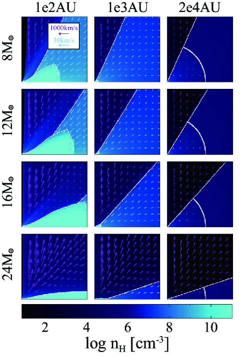
Figure 1.— Evolutionary sequence of density, $n_{\rm H}$, and velocity fields around protostars of mass $m_{*}=8,~{}12,~{}16,{\rm~{}and~{}}24M_{\odot}$ forming from a core with initial properties $M_{c}=60M_{\odot},~{}\Sigma_{\rm cl}=1\>{\rm g~{}cm^{-2}},$ and $\beta_{c}=0.02$ (model A08, A12, A16, and A24). Three spatial scales, successively zooming out from the protostar, are shown from left to right. In each panel, the protostar is at the lower left corner, the horizontal axis lies on the disk midplane and the vertical axis along the outflow axis. The velocity fields are shown by arrows (purple for the outflow; light-blue for the infalling envelope; note the different velocity scales). The initial core radius, i.e., its boundary with the clump, and the boundaries of disk, envelope and outflow are indicated by white lines.

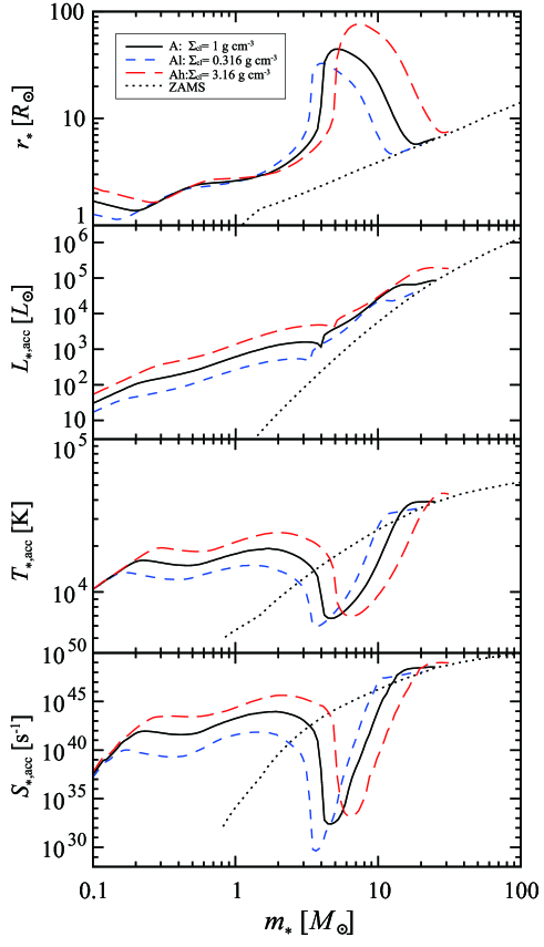
Figure 2.— Evolutionary sequences of $r_{*}$, $L_{*,\rm acc}$, $T_{*,\rm acc}$, and $S_{*,\rm acc}$ versus protostellar mass (top to bottom) for protostars forming from $M_{c}=60M_{\odot}$ and $~{}\beta_{\rm c}=0.02$. The black solid line shows the case with $\Sigma_{\rm cl}=1\>{\rm g~{}cm^{-2}}$, while blue dashed and red long-dashed lines show the $\Sigma_{\rm cl}=0.316$ and $3.16\>{\rm g~{}cm^{-2}}$ cases, respectively. The ZAMS properties are shown by the dotted lines.

We calculate the photoionization structure and present synthetic observations in the context of the Turbulent Core Accretion Model of MT03. We use a series of models of protostellar evolution and surrounding gas structure constructed by ZTH14, which self-consistently include the evolution of the protostar and disk formed from a rotating parent core embedded in a particular clump environment, and mass accretion regulated by disk-wind outflows. We note that these models are highly idealized in that they assume axisymmetry about a single protostar, while real objects will be more irregular, especially if the initial core is highly turbulent, and may be forming in a cluster environment with other protostars in the vicinity. Even if there is a relatively ordered and isolated core that is collapsing to a central disk, this collapse may lead to binary or low-order multiple star formation. Still, by first presenting the simplest case of formation of an isolated massive protostar, we can then see how relevant such models are as approximations to real systems.

Here we briefly review the evolution of the protostar and its surrounding gas structures. The initial core is assumed to be spherical and in near virial equilibrium via support by turbulence and/or magnetic fields. The evolutionary track of a core is determined by three environmental initial conditions: core mass $M_{\rm c}$, mass surface density of ambient clump $\Sigma_{\rm cl}$ (which sets surface pressure of the core), and ratio of the core’s initial rotational to gravitational energy $\beta_{c}$. We fix the rotational parameter $\beta_{c}=0.02$ as a typical value from observations of lower-mass cores (Goodman et al., 1993; Li et al., 2012; Palau et al., 2013). The core density structure is described by a power law in spherical radius, $\rho\propto r^{-k_{\rho}}$. Values of $k_{\rho}\simeq 1.3$–$1.6$ are inferred from observations of dense cores in Infrared Dark Clouds (IRDCs) (Butler & Tan, 2012; Butler et al., 2014). We adopt $k_{\rho}=1.5$ as a fiducial value, following MT03. Then, the radius of a core is $R_{c}=1.2\times 10^{4}(M_{c}/60M_{\odot})^{1/2}(\Sigma_{\rm cl}/1~{}{\rm g\>cm^{-2}})^{-1/2}{\rm AU}$. Since the core is in pressure equilibrium with the surrounding clump, it is more compact for higher $\Sigma_{\rm cl}$.

Table 1 presents the parameter sets of $(M_{c},~{}\Sigma_{\rm cl})$ for which we study the ionization structures. These are the same as studied by ZTH14. We refer to model group A as a fiducial group with $M_{c}=60M_{\odot}$ and $\Sigma_{\rm cl}=1~{}{\rm g\>cm^{-2}}$. We also investigate high- and low-$\Sigma_{\rm cl}$ cases, model groups Al and Ah, and $M_{c}=120\>M_{\odot}$ and 240$M_{\odot}$ cases, as model groups B and C, respectively.

The core undergoes inside-out collapse (Shu, 1977; McLaughlin & Pudritz, 1997) with the effect of rotation described with the solution by Ulrich (1976) (see also Tan & McKee, 2004). Given the high accretion rates associated with collapse of dense cores, the protostellar disk is expected to be massive and self-gravitating such that angular momentum may be transported by torques due to, e.g., spiral arm structures. Considering this efficient angular momentum transfer, the mass ratio between disk and protostar is set to be a constant $f_{d}=m_{d}/m_{*}=1/3$ (e.g., Kratter et al., 2008). The disk structure is described by a standard $\alpha$-viscosity disk model (Shakura & Sunyaev, 1973), but also including the effects of infall and outflow (conservations of mass and angular momentum). The temperatures at the midplane are evaluated by vertical energy balance, and the vertical structure of the disk is determined by this temperature. The disk surface is set by assuming continuity with the density structure of the outflow. More details about the disk model are described in Zhang et al. (2013).

The mass accretion rate onto the forming protostar $\dot{m}_{*}$ is

$$\dot{m}_{*} = 9.2\times 10^{-4}\frac{\epsilon_{*}}{\overline{\epsilon}_{*}^{0.5}}\left(\frac{m_{*}}{M_{\rm c}}\right)^{0.5}$$ (1)

$$\times\left(\frac{M_{c}}{60M_{\odot}}\right)^{3/4}\left(\frac{\Sigma_{\rm cl}}{1~{}{\rm g\>cm^{-2}}}\right)^{3/4}M_{\odot}\>{\rm yr}^{-1},$$

where $\epsilon_{*}(t)$ and $\overline{\epsilon}_{*}(t)$ are the instantaneous and averaged star formation efficiencies. The instantaneous star formation efficiency ${\epsilon}_{*}$ is the ratio of the accretion rate onto the star to the idealized spherical infall rate from the initial cloud core in the absence of feedback: a certain percentage of infalling material is swept up by the disk wind (see next paragraph) and a fraction, $f_{d}$, of the accreted mass remains in the disk during the protostellar phase. The averaged star formation efficiency $\overline{\epsilon}_{*}$ is the ratio of the stellar mass to the idealized collapsed mass of the initial cloud core at the same stage of infall in the absence of feedback. The accretion rate is high for high clump mass surface densities, since high $\Sigma_{\rm cl}$ results in a more compact core and thus shorter collapse time. Also, this formula indicates that in the no-feedback limit of $\epsilon_{*}=\overline{\epsilon}_{*}=1$, the accretion rate increases with time, i.e., as $m_{*}^{0.5}$ (see MT03).

The magnetically driven bipolar outflows sweep up part of the core and thus help set the star formation efficiency $\epsilon_{*}$. The density and velocity distributions of the outflow are described by a semi-analytic disk wind solution that is modified from the centrifugally driven outflow model of Blandford & Payne (1982) (for details, see Zhang et al., 2013, and ZTH14). The mass loading rate of the wind is proportional to the mass accretion rate, with a ratio $f_{w}=0.1$ assumed as a typical value (Königl & Pudritz, 2000). The velocity is as high as $\sim 1000\>{\rm km\>s^{-1}}$ near the rotation axis and then smoothly decreases at lower latitudes. This outflow velocity structure represents features of both a collimated fast jet and a wider-angle, slower wind. The opening angle of the outflow cavity $\theta_{\rm w,esc}$ is estimated following the method of Matzner & McKee (2000): if the outflow momentum is strong enough to accelerate the core material to its escape speed, the outflow extends in that direction. The outflow momentum, ${p}_{w}$, is evaluated by integrating the momentum rate $\dot{p}_{w}$ over time. The momentum injection rate is typically $\dot{p}_{w}\simeq(0.15$ – $3)\times\dot{m}_{*}v_{K*}$ in our model, where $v_{K*}\simeq 440(m_{*}/10M_{\odot})^{1/2}(r_{*}/10R_{\odot})^{-1/2}{\rm\>km\>s^{-1}}$ is the Keplerian speed at the stellar radius. This process sets the star formation efficiency $\epsilon_{*}$ (and also $\overline{\epsilon}_{*}$). For more details of the outflow model and the evaluation of the star formation efficiency, see Zhang et al. (2013) and ZTH14.

Figure 1 shows an example of the evolution of the density and velocity structures in the fiducial case. The gradual opening-up of the outflow can be seen at the scale of $2\times 10^{4}\>{\rm~{}AU}$ with typical outflow velocity of $100\>$–$\>500\>{\rm\>km\>s^{-1}}$ which is high near the axis. This leads to a decrease in the instantaneous star formation efficiency. At the end of accretion in this model, the stellar mass reaches $26\>M_{\odot}$ and the final averaged star formation efficiency is $\overline{\epsilon}_{*f}=26M_{\odot}/60M_{\odot}=0.43$. For the different models, the averaged final star formation efficiencies are similar, with a range of $\overline{\epsilon}_{*f}=0.34\>$–$\>0.52$. While we expect the momentum flux from protostellar outflows to be the dominant source of feedback, we note that additional feedback processes due to ionization, (line-driven) stellar winds and radiation pressure are not yet included in our modeling, so the above efficiencies may be somewhat overestimated. The growth of the disk radius can be seen in the panels showing the scale of $100\>{\rm AU}$. Note, partly for the reason of being near the end of its accretion phase and having a relatively low accretion rate, the disk in the $24\>M_{\odot}$ case appears relatively thin compared to earlier stages (ZTH14). On the $100\>{\rm AU}$ scales, we also see the narrow, inner, on-axis cavity of the disk wind, which is set to have zero (i.e., negligible) density. This cavity is too thin to see in the larger scale panels, but it is resolved by the logarithmic grid spacing.

The evolution of the protostar depends on its accretion history. ZTH14 calculated the protostellar properties with a detailed stellar evolution model by Hosokawa & Omukai (2009) and Hosokawa et al. (2010), self-consistently adapted to the Turbulent Core Model accretion rates. When the flow reaches the stellar surface, the accretion energy, $L_{\rm acc}=Gm_{*}\dot{m}_{*}/(2r_{*})$, is released there. Following ZTH14, we treat this accretion luminosity and the internal stellar luminosity as being emitted isotropically with a single effective temperature, $T_{\rm*,acc}$, i.e., $L_{\rm*,acc}=L_{*}+L_{\rm acc}=4\pi r_{*}^{2}\sigma T_{\rm*,acc}^{4}$. We will refer to $T_{\rm*,acc}$ as the stellar effective temperature. ZTH14 also included the effects of the accretion energy released at the disk surfaces in the dust temperature calculation. However, in this study, we neglect the ionizing photons from the disk surface, since its surface temperature is not high enough to emit significant amounts of ionizing flux. If the protostar rotates at almost its breakup velocity, it distorts the structure of the star. This effect leads to nonuniform surface temperatures: the polar region is hotter than the equatorial region (Meynet et al., 2010). However, the degree of rotation of massive protostars is quite uncertain, and thus for simplicity we adopt a spherical model with a single surface temperature as a first approximation.

Figure 2 shows the evolution of protostellar properties with protostellar mass: the stellar radius, luminosity and effective temperature were calculated by ZTH14, while the evaluation of ionizing flux will be described in §2.2.1. In the fiducial case with $M_{c}=60~{}M_{\odot}$ and $\Sigma_{\rm cl}=1\>{\rm g~{}cm^{-2}}$, the stellar radius reaches a maximum at $m_{*}\simeq 5\>M_{\odot}$ when the Kelvin-Helmholz time becomes as short as the accretion time, after which the protostar is able to begin contraction towards the zero-age main sequence (ZAMS) (Hosokawa & Omukai, 2009). Due to this variation in radius, the effective temperature increases strongly for $m_{*}\gtrsim 5M_{\odot}$. Comparing to the fiducial case, the mass at which the stellar radius has a maximum is larger in the higher $\Sigma_{\rm cl}$ case and smaller in the lower $\Sigma_{\rm cl}$ case. This is because a higher $\Sigma_{\rm cl}$ causes higher accretion rates (eq. 1), which make the accretion timescale shorter and also lead to increased swelling of the protostar.

2.2. Photoionization

2.2.1 Ionizing photon luminosity

The total stellar H-ionizing photon luminosity $S_{*,\rm acc}$ is evaluated as

$$S_{\rm*,acc}=\int_{\nu_{0}}^{\infty}\frac{L_{\nu,\rm*,acc}}{h\nu}d\nu,$$ (2)

where $\nu$ is the frequency, $\nu_{0}$ is the Lyman limit frequency, and $L_{\nu,{\rm*,acc}}$ is the luminosity per frequency interval (i.e., the stellar spectrum). The stellar atmosphere model of Castelli & Kurucz (2004) is adopted to estimate $L_{\nu,{\rm*,acc}}$, which covers wide ranges of effective temperature and surface gravity. The variation of ionizing luminosity is sensitive to the effective temperature and varies by orders of magnitude (bottom panel of Figure 2). In the fiducial case of group A, the ionizing luminosity is as small as $3\times 10^{32}\>{\rm~{}s^{-1}}$ at $4.7\>M_{\odot}$, and quickly increases to $10^{48}\>{\rm~{}s^{-1}}$ or larger in the Kelvin-Helmholz contraction phase. Even at the same mass of $12\>M_{\odot}$, the ionizing luminosity of model Ah12 is five orders of magnitude smaller than that of model Al12. Therefore, the accretion history and the detailed stellar evolution calculation are essential to study the ionization structure. We note that the obtained ionizing photon luminosities are somewhat lower than those in Figure 2 of Tan et al. (2014) due to improved calculation of the effects of line blanketing.

2.2.2 Transfer of ionizing photons

We calculate the extent of the ionized regions using our previously developed radiative transfer code (Tanaka et al., 2013), which allows a treatment of both direct and diffuse ionizing radiation fields. We consider only the ionization of Hydrogen, ignoring Helium and other elements. If the stellar effective temperature is high, $T_{\rm*,acc}>40,000{\rm K}$, we would underestimate the electron density by about $10\%$ due to singly ionized Helium, which would then enhance free-free emission by about $20\%$.

The gray approximation for the photoionization calculation is adopted, where the frequency of ionizing photons is represented by the mean value. The equation of radiative transfer along a ray is

$$\frac{dI}{ds}=-x_{\rm I}n_{\rm H}\sigma_{\rm H}I+\alpha_{1}x_{\rm II}^{2}n_{\rm H}^{2}\frac{\langle h\nu\rangle}{4\pi}$$

$$-n_{\rm H}\sigma_{\rm d,a}I+n_{\rm H}\sigma_{\rm d,s}(J-I),$$ (3)

where $n_{\rm H}$ is the number density of hydrogen nuclei, $I$ is the irradiance intensity, $J=\int Id\Omega/4\pi$ is the mean intensity, $\langle h\nu\rangle$ is the mean energy of ionizing photons, $\sigma_{\rm H}$ is the mean photoionization cross-section of the Hydrogen atom, $\alpha_{1}$ is the radiative recombination coefficient to the ground state, $x_{\rm I}$ and $x_{\rm II}$ are neutral (atomic) and ionized fractions of H, $\sigma_{\rm d,a}$ and $\sigma_{\rm d,s}$ are absorption and scattering cross sections of dust grains per H nucleon. The first term of the right-hand side represents the consumption of ionizing photons by neutral Hydrogen, the second term describes the re-emission of ionizing photons by recombinations directly to the ground state, and the third and fourth terms correspond to absorption and scattering by dust grains, respectively. The local ionization fraction of H, $x_{\rm II}$, is calculated from the balance between photoionization, recombination and advection,

$$\nabla\cdot\left(n_{\rm H}x_{\rm II}{\bf v}\right)=\frac{4\pi x_{\rm I}n_{\rm H}\sigma_{\rm H}J}{\langle h\nu\rangle}-\alpha_{\rm A}x_{\rm II}^{2}n_{\rm H}^{2},$$ (4)

where ${\bf v}$ is the velocity of the disk wind gas, $\alpha_{\rm A}$ is the recombination coefficient for all levels (so-called case A). The advection term on the left-hand side of this equation can be especially important near the ionization boundary. The recombination rates, $\alpha_{1}$ and $\alpha_{\rm A}$, are functions of temperature of the ionized gas. The mean values of the photon energy and Hydrogen cross-section are evaluated from the stellar spectra for each model,

$$\langle h\nu\rangle = \frac{1}{S_{*,\rm acc}}\int_{\nu_{0}}^{\infty}L_{\nu,{\rm*,acc}}d\nu,$$ (5)

$$\sigma_{\rm H} = \frac{1}{S_{*,\rm acc}}\int_{\nu_{0}}^{\infty}\sigma_{\rm H,\nu}\left(\frac{L_{\nu,{\rm*,acc}}}{h\nu}\right)d\nu,$$ (6)

where $\sigma_{\rm H,\nu}$ is the frequency dependent cross-section of the Hydrogen atom. We adopt the fitting formulas from Draine (2011) for the recombination rates $\alpha_{1}$ and $\alpha_{A}$, and the Hydrogen cross-section $\sigma_{\rm H,\nu}$. The absorption and scattering properties of dust in these H II regions are quite uncertain. We adopt $\sigma_{\rm d,a}$ and $\sigma_{\rm d,s}$ equal to zero in regions where the temperature history has exceeded the dust destruction temperature (1,400 K) in the thermal radiation calculation by ZTH14 (i.e., there is a dust-free inner region of the disk wind), and elsewhere they are fixed at $10^{-21}~{}{\rm cm^{2}}$ from a typical value of the diffuse interstellar medium (Weingartner & Draine, 2001). The effect of variation of dust grain properties, i.e., sizes, abundances, compositions, is deferred to a future paper.

We conduct axisymmetric two dimensional calculations to solve equations (3) and (4), using our developed ray-tracing radiative transfer code. In the previous work of Tanaka et al. (2013), the code solved the transfer equation by the method of short characteristics, which involves only the cells next to the point under consideration (Stone et al., 1992). Here, we update the code implementing the method of long characteristics. With this method, the transfer problem is solved along the rays from the domain boundary to each point, which leads to less numerical diffusion and treats the diffuse radiation more accurately than the short characteristics method. The computational domain is a cylindrical region with radial and vertical coordinates $R\leq 20,000\>{\rm~{}AU}$ and $Z\leq 20,000\>{\rm~{}AU}$, assuming equatorial plane symmetry. The ionizing photon source is a sphere located at $(R,Z)=(0,0)$ with a radius of $r_{*}$, which represents the accreting star. We denote the distance from the center of the star as $r=\sqrt{R^{2}+Z^{2}}$. The spatial grids for radial and vertical directions are set to be spaced logarithmically since the inner region has finer structures. The entire computational domain is resolved with a $256\times 256$ grid. The radiation intensity $I$ is a function of location and also direction: $I=I(R,Z,\theta,\phi)$ where $\theta$ and $\phi$ are the polar and azimuthal angles, respectively. The radiation emitted from the vicinity of the star has very fine angular structure when it reaches the outer boundary, i.e., $\delta\theta\sim\delta\phi\sim r_{*}/r_{\rm max}\sim 10^{-6}$. To resolve these fine structures while still saving computational costs, the angular resolutions of $\theta$ and $\phi$ are configured to vary depending on location $(R,\;Z)$. In the $\theta$ direction, the radiation arriving from directions with $\theta\simeq\tan^{-1}(R/Z)$, which comes from the vicinity of the star, is resolved with a high resolution of $\Delta\theta\ll r_{*}/r$, while the radiation arriving from $\theta\simeq\tan^{-1}(R/Z)+\pi/2$ is resolved by $\Delta\theta\simeq 10^{-2}$. In the $\phi$ direction, based on the tangential plane method (Stone et al., 1992), the radiation emitted from near the axis and from the opposite direction, $\phi\simeq 0$ and $\pi$, is resolved with high resolution of $\Delta\phi\ll r_{*}/r$, while the radiation from $\phi\simeq\pi/2$ is resolved by $\Delta\phi\simeq 10^{-2}$. We also conduct resolution tests for the fiducial case with grids of $128\times 128$ and $330\times 330$. The obtained ionized structures are consistent at these resolutions and free-free fluxes change by less than $6\%$ at radio frequencies from $0.3\>$–$\>300\rm GHz$.

In this first work we study the photoionization of the disk wind, and do not allow photoionization of gas in the disk or infall envelope components of the model. Such photoionization would enhance the mass loss rate that is being injected into the disk wind, i.e., by photoevaporation, and would thus change its density structure and also the star formation efficiency. This feedback of photoevaporation will be discussed in a future paper.

2.2.3 Temperature of the ionized gas

The temperature of the ionized gas is important to evaluate recombination rates and to study free-free emission for observational diagnostics. The photoionized gas temperature is regulated to around $10,000{~{}\rm K}$ by the balance of heating and cooling processes. The dominant heating process is photoionization and the main cooling processes are radiative cooling of collisionally excited metal lines, recombination of H, and free-free emission.

It is computationally expensive to take into account all heating and cooling processes at every step of the radiative transfer calculation, and thus here we introduce an approximate treatment. The heating rate by photoionization depends on the stellar spectrum. Also, heating and cooling rates are both mostly sensitive to the density. Therefore, we treat the photoionized gas temperature, for each stellar model, as a function of the local density, i.e., $T(n_{\rm H})$. We evaluate $T(n_{\rm H})$ from the volume average temperature of static H II regions with uniform densities in the range $n_{\rm H}=10\>$–$\>10^{11}\>{\rm cm^{-3}}$ using version 13.03 of CLOUDY (Ferland et al., 2013). This approximate approach is appropriate since a uniform density H II region for each stellar model is almost isothermal as shown below. It should be noted that the ionized gas temperature is also sensitive to the metallicity of the gas, and we assume solar metallicity in this study.

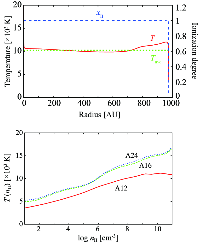
Figure 3.— Top: Radial structure of an H II region with an uniform density of $n_{\rm H}=10^{6}\>{\rm cm}^{-3}$ formed by the radiation of the stellar model of A24. The radial structures of temperature, $T$, (solid) and ionization degree of H, $x_{\rm II}$, (dashed) are shown. The volume averaged temperature of $T_{\rm ave}=10,225{\rm~{}K}$ is also indicated (dotted). Bottom: Ionized gas temperature as a function of density, $T(n_{\rm H})$, which is set equal to the volume-averaged photoionized gas temperature, $T_{\rm ave}(n_{\rm H})$. Results are shown for stellar models A12, A16, and A24.

The top panel of Figure 3 shows the radial structure of an H II region with uniform density of $n_{\rm H}=10^{6}\>{\rm~{}cm^{-3}}$ formed by the stellar radiation of the stellar model A24. It can be seen that the H II region has a sharp edge at $960\>{\rm AU}$ where the ionization degree drops from near unity to near zero. The temperature is almost isothermal in the ionized region. We evaluate the typical photoionized gas temperature at $n_{\rm H}=10^{6}\>{\rm cm^{-3}}$ as being $10,225{\rm K}$ from the volume average of this temperature for this stellar model.

In this way, we obtain photoionized gas temperatures over the density range of $n_{\rm H}=10\>$–$\>10^{11}\>{\rm cm^{-3}}$ for each stellar model. The bottom panel of Figure 3 shows the photoionized gas temperature as functions of density, $T(n_{\rm H})=T_{\rm ave}(n_{\rm H})$, for the stellar models A12, A16, and A24. The temperatures of all models are around $5,000$–$15,000{\rm K}$ for orders of magnitude of density variation. The temperature is typically higher at higher density. This is because the cooling is suppressed if the density exceeds the critical density of some of the cooling lines. We adopt these averaged temperatures to set $T(n_{\rm H})$ as the local temperature of the ionized gas in our radiative transfer calculations.

Since the adopted temperature is evaluated based on static H II region calculations, adiabatic cooling has not been included in this study. The adiabatic cooling rate, $\Lambda_{\rm ad}\simeq 2.5\nabla\cdot(n_{\rm H}k_{\rm B}T{\bf v})$, is proportional to $\sim n_{\rm H}/r$. On the other hand, the radiative cooling rates in ionized regions are almost proportional to the square of density. Since the density gradient in the disk wind is as steep as $d\log n_{\rm H}/d\log r\sim-1.5$ to $-2$, adiabatic cooling may not be negligible in low density regions far from the star. We compare the adiabatic cooling rate to the cooling rate evaluated by the static calculations. In the fiducial model of A16, adiabatic cooling would be $>20\%$ of total cooling rate when $n_{\rm H}<10^{4}\>{\rm cm^{-3}}$ and $r>1000\>{\rm AU}$. As we will see in §3.2.1, the free-free flux at frequencies lower than $1{\>\rm GHz}$ is mainly provided from $r>1000{\rm AU}$. Therefore, we note that the SEDs obtained by our simplified modeling would be overestimated somewhat at $\lesssim 1\>{\rm GHz}$.

2.3. Observables

2.3.1 Free-free emission

Using the obtained structures of the photoionized outflow, we estimate the free-free radio continuum emission. The equation of transfer for free-free emission is

$$\frac{dI_{\nu,{\rm ff}}}{ds}=-\kappa_{\nu,{\rm ff}}\left(I_{\nu,{\rm ff}}-B_{\nu}\right),$$ (7)

where $I_{\nu,{\rm ff}}$ and $\kappa_{\nu,{\rm ff}}$ are the intensity and opacity of free-free emission, and $B_{\nu}(T)$ is the Planck function. The opacity due to free-free absorption is given by

$$\kappa_{\nu,{\rm ff}}=\frac{4}{3}\left(\frac{2\pi}{3}\right)^{1/2}\frac{e^{6}}{m_{e}^{3/2}hc}\frac{n_{\rm H}^{2}x_{\rm HII}^{2}}{\sqrt{k_{B}T}}$$

$$\times\left[\frac{1-\exp{\left(-h\nu/k_{B}T\right)}}{\nu^{3}}\right]g_{\rm ff},$$ (8)

where $e$ and $m_{e}$ are the charge and mass of the electron, $h$ is the Planck constant, $c$ is the speed of light, $k_{B}$ is the Boltzmann constant, and $g_{\rm ff}(\nu,T)$ is the Gaunt factor for free-free emission. The observed flux density is obtained by integrating over source solid angle of $\Omega_{s}$,

$$F_{\nu,{\rm ff}}=\int_{\rm\Omega_{s}}I_{\nu,{\rm ff}}\cos(\theta-\theta_{\rm view})d\Omega=\int_{\rm\Omega_{s}}I_{\nu,{\rm ff}}d\Omega,$$ (9)

where $\theta_{\rm view}$ is the viewing inclination measured from the outflow axis. In the last formula, we assumed that the distance is much farther than the object size, i.e., $\theta-\theta_{\rm view}\lesssim 20,000{\rm AU}/1{\rm\>kpc}\ll 1$. In this study, for quantitative results, we assume protostars are located at a distance of $1\>{\rm~{}kpc}$, and total fluxes are obtained by integrating over a radius out to $10^{4}\>{\rm~{}AU}$ from the central star (for all our models this region dominates the total flux from free-free emission). The free-free emission is typically observed at $\nu\simeq 0.1$–$100\>{\rm~{}GHz}$, while the thermal dust emission would usually be dominant at higher frequencies. However, for completeness, we calculate free-free emission over the frequency range of $\nu=10^{-1}$–$10^{7}{\rm~{}GHz}$.

2.3.2 Hydrogen recombination lines

We also evaluate the HRL emission from the photoionized outflow. Considering a H$n\alpha$ line, i.e., the line from the transition $n+1\rightarrow n$, the opacity is

$$\kappa_{\nu,\rm HRL} = n_{n}\frac{\lambda_{n}^{2}}{8\pi}\left(\frac{n+1}{n}\right)^{2}$$ (10)

$$\times A_{n+1,n}\left(1-e^{-h\nu_{n}/k_{B}T}\right)\phi_{\nu},$$

where $\phi_{\nu}$ is the normalized line profile ($\int\phi_{\nu}d\nu=1$), $n_{n}$ is the population number in energy level $n$, $A_{n+1,n}$ is the Einstein coefficient of spontaneous emission, and $h\nu_{n}$ and $\lambda_{n}=c/\nu_{n}$ are the energy and wavelength of the H$n\alpha$ transition, respectively. Here, for simplicity, we assume the case of local thermodynamic equilibrium (LTE). However we note that, in the particular case of the massive star MWC 349A, maser amplification of HRLs are observed and thus non-LTE effects can be important (for modeling of MWC 349A including non-LTE effects, see Báez-Rubio et al., 2013).

The transfer for the total intensity, $I_{\nu,\rm ff,HRL}$, i.e., the sum of the free-free and HRL emission, is

$$\frac{dI_{\nu,{\rm ff,HRL}}}{ds} = -(\kappa_{\nu,{\rm ff}}+\kappa_{\nu,{\rm HRL}})\left(I_{\nu,{\rm ff,HRL}}-B_{\nu}\right),$$ (11)

and the total observed flux is

$$F_{\nu,{\rm ff,HRL}} = \int_{\rm\Omega_{s}}I_{\nu,{\rm ff,HRL}}\cos(\theta-\theta_{\rm view})d\Omega$$ (12)

$$= \int_{\rm\Omega_{s}}I_{\nu,{\rm ff,HRL}}d\Omega.$$

Here, we assumed that the source distance is greater than its size as in equation (9). We evaluate the HRL flux as the excess from the continuum flux at $\nu_{n}$, i.e., $F_{\nu,{\rm HRL}}=F_{\nu,{\rm ff,HRL}}-F_{\nu_{n},{\rm ff}}$. Of course, observationally it is not possible to observe the free-free flux exactly at $\nu_{n}$ since the line exists there and we cannot divide the total flux into two components. However, the value of $F_{\nu_{n},{\rm ff}}$ is still able to evaluated from the far tail of the line profile or from interpolating from continuum observations at other frequencies. Since the typical line width is $\Delta\nu/\nu_{n}\sim v/c<10^{-3}$ and the typical free-free emission spectral index in this study is $0\lesssim p\lesssim 1$, the variation of the continuum flux in this width is less than $0.1\%$. Thus, it is safe to assume the continuum is constant over the line width. In this paper we will illustrate these results with the H$40\alpha$ line at $99\>{\rm GHz}$. The flux ratio is typically $F_{\nu,{\rm HRL}}/F_{\nu,{\rm ff}}\sim 0.1$ for the H$40\alpha$ line in our models.

We assume that locally the gas has a Maxwellian velocity distribution, ignoring the intrinsic width of the line relative to the thermal and bulk-motion broadening. The velocity dispersion of Hydrogen is $\sigma_{v}=\sqrt{k_{\rm B}T/m_{\rm H}}$, and the corresponding dispersion in frequency is $\sigma_{\nu}=(\sigma_{v}/c)\nu_{n}$. The local normalized line profile $\phi_{\nu}$ combining the bulk gas velocity along the line of sight, $v$, is

$$\phi_{\nu}=\frac{1}{\sqrt{2\pi\sigma_{\nu}^{2}}}\exp\left[-\frac{\left\{(1+v/c)\nu-\nu_{n}\right\}^{2}}{2\sigma_{\nu}^{2}}\right].$$ (13)

The frequency $\nu$ observationally represents a radial velocity of $(1-\nu/\nu_{n})c$.

2.4. Escape fraction of ionizing photons

As we will see in next section, the ionized region, after initial early expansion, becomes unconfined in the radial direction along the outflow axis. Thus, some fraction of the ionizing photons escapes from the protostellar core and can ionize the surrounding, ambient clump gas, which may be forming a stellar cluster. Although the main focus of this work is the ionized structure of disk winds and their observational properties, ambient gas ionization is also important for its effect on star cluster formation and production of additional radio emission. Therefore, we provide estimates of the ionization of escaping photons and radio emission from the ionized clump gas.

The escape fraction of ionizing photons depends on the polar angle $\theta$, i.e., in response to the ionized disk wind structure. We calculate the escape fraction as

$$f_{\rm esc}(\theta)=\frac{4\pi r^{2}F_{r,\rm out}(\theta)}{S_{\rm*,acc}\langle h\nu\rangle},$$ (14)

where $F_{r,\rm out}$ is the radial energy flux of ionizing photons at the outer boundary, i.e., $R=20,000\>{\rm AU}$ or $Z=20,000\>{\rm AU}$. We note that the escape fraction is insensitive to the choice of the radius at which escape is defined as long as it is significantly larger than the disk radius. Integrating $f_{\rm esc}$ over the boundary, we obtain the total escape fraction,

$$\overline{f}_{\rm esc}=\frac{1}{4\pi}\int f_{\rm esc}(\theta)d\Omega.$$ (15)

3. Results

3.1. Structure and evolution of the photoionized outflow

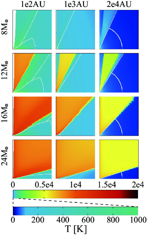
Figure 4.— Evolutionary sequences of the photoionized outflows of model group A. The color scale shows the temperature of the photoionized and neutral regions. The white regions seen close to the vertical axes in the $100{\rm\>AU}$-scale panels (left column) are disk wind inner cavities, where the gas density is negligible (formally zero) and the ionizing photon can travel freely. As in Figure 1, the core scale and the boundaries between disk, core envelope, outflow and clump are shown by white lines.

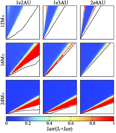
Figure 5.— The radiation fields for model group A. The color scale shows the fraction of diffuse radiation in the ionized region (the white region is neutral). Black lines indicate the disk/envelope boundaries with the disk wind.

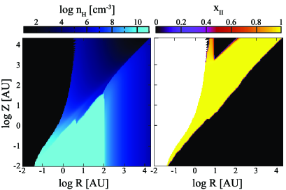
Figure 6.— The structures of density $n_{\rm H}$ (left) and ionization degree $x_{\rm II}$ (right) for model A16 in logarithmic scale. The white region in the right panel is the inner hole where the ionization degree cannot be defined due to the zero density. However, the ionizing photons travels this inner hole freely. Note that the stellar radius is $r_{*}=6.4R_{\odot}=0.03{\>\rm AU}$ for this model.

First we report results of the fiducial case, model group A. Figure 4 shows the evolution of the photoionized structure. The high temperature region with $\sim 10^{4}\>{\rm K}$ is the photoionized gas, i.e., the H II region, and elsewhere is neutral gas (with temperatures calculated from the ZTH14 radiative transfer models; note, we expect there would be some localized changes to the ZTH14 results for the neutral gas due to the presence of the H II region and its associated photodissociation region (PDR), but we ignore those here—the PDR region will be considered in a future paper). Note that the white regions seen along the rotation axes in the $100{\>\rm AU}$-scale panels are disk wind inner cavities, where the density is negligible (formally zero in these models since we do not include a line-driven wind from the stellar surface) and thus where ionizing photons can travel freely. The ionized gas temperature is slightly higher in the inner region of the disk wind due to the higher density (see Fig. 3). When $m_{*}\leq 8M_{\odot}$, the ionizing photon luminosity is too low to ionize the disk wind. As the ionizing luminosity increases with mass, the photoionized region is formed. When $m_{*}=12\>M_{\odot}$, the photoionized region is confined to intermediate zenith angles of $10\arcdeg\lesssim\theta\lesssim 30\arcdeg$. This is because densities are higher near the outflow axis at $\theta<10\arcdeg$ and near its launching zone for $\theta\gtrsim 30\arcdeg$. Since the radial density gradient in the outflow is typically steeper than $r^{-1.5}$, the photoionized region is not confined in the radial direction and breaks out. The opening angle of the photoionized region increases as the protostellar mass grows. The ionized region eventually reaches the flared disk surfaces, however some parts of the disk wind remain neutral due to the shielding by the inner disk and disk wind even though the diffuse radiation is considered. Therefore, photoevaporation from the disk surface is suppressed, while photoevaporation from the envelope may still be efficient.

The ionizing radiation has two components: one is the direct stellar radiation and the other is the diffuse radiation from recombinations to the ground state and dust scattering. Figure 5 shows the fraction of diffuse radiation, $J_{\rm diff}/(J_{*}+J_{\rm diff})$, at each evolutionary stage. The direct radiation dominates over most of the outflow. However, in some locations, due to the direct radiation being shielded by the inner disk at $\ll 10^{2}\>{\rm AU}$, the diffuse radiation becomes more important, i.e., near the ionized-neutral boundary, e.g., as seen in model A24. In this way, as suggested by Hollenbach et al. (1994), the diffuse radiation is important to determine the structure of the H II region and rates of photoevaporation from the neutral components. For these reasons, accurate treatment of the radiative transfer including the diffuse component is necessary.

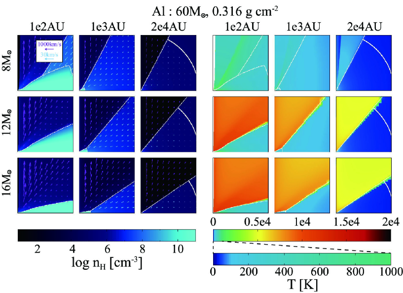
Figure 7.— The evolution of density (left) and photoionization (as revealed by gas temperature, $T$) (right) structures for model groups Al ($M_{c}=60\>M_{\odot},\>\Sigma_{\rm cl}=0.316{\rm g\>cm^{-2}}$).

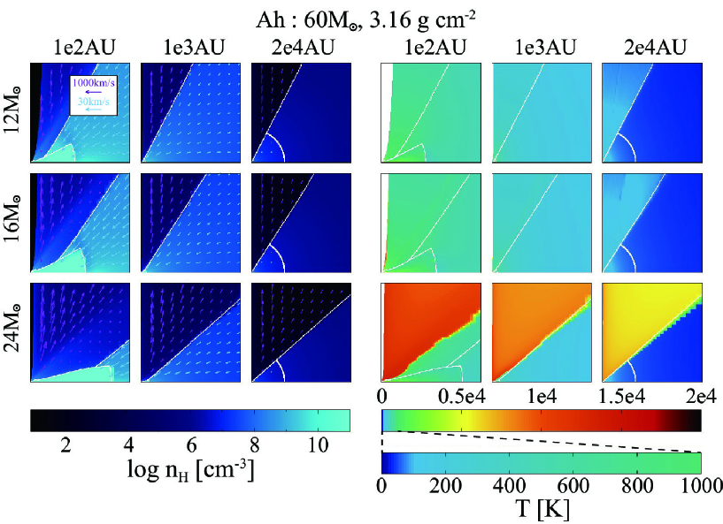
Figure 8.— The evolution of density (left) and photoionization (as revealed by gas temperature, $T$) (right) structures for model groups Ah ($M_{c}=60\>M_{\odot},\>\Sigma_{\rm cl}=3.16{\rm g\>cm^{-2}}$).

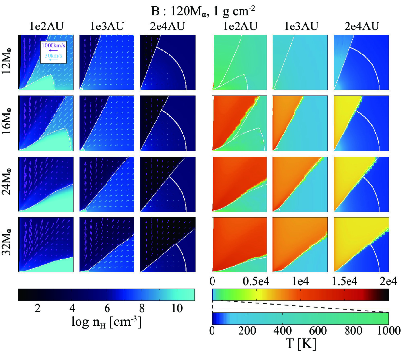
Figure 9.— The evolution of density (left) and photoionization (as revealed by gas temperature, $T$) (right) structures for model groups B ($M_{c}=120\>M_{\odot},\>\Sigma_{\rm cl}=1{\rm g\>cm^{-2}}$).

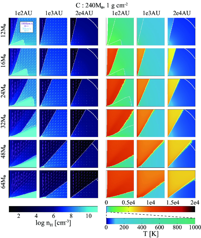
Figure 10.— The evolution of density (left) and photoionization (as revealed by gas temperature, $T$) (right) structures for model groups C ($M_{c}=240\>M_{\odot},\>\Sigma_{\rm cl}=1{\rm g\>cm^{-2}}$).

To illustrate the structure near the rotation axis, Figure 6 shows the density and ionization fraction of model A16 with a logarithmic scale. The disk wind inner cavity, with zero density inside its innermost streamline, is seen as a very collimated structure with $\theta<2\times 10^{-4}$ at $Z=20,000\>{\rm AU}$ (the black region in left panel and the white region in right panel). The density is high along the inner edge of the outflow. Due to the shielding by this high density inner wall, the gas in the region at high latitude with $R\sim 10$–$100{\rm\>AU}$ and $Z\gtrsim 1000{\rm\>AU}$ remains neutral. This shielding is the same mechanism seen in model A12 in which the neutral region is at $\theta\lesssim 10\arcdeg$. The strip of ionized gas entering this neutral region is caused by high velocity advection near the axis (eq. 4). These thin structures near the axis are sensitive to our adoption of an idealized axisymmetric model. In reality, the outflow winds are not expected to be perfectly axisymmetric. For example, the jet in IRAS 16547-4247 appears to undergo precession (Rodríguez et al., 2008). However, the idealized structures in our model illustrate the wind shielding effect and also demonstrate the accuracy of our numerical calculation even at such fine angular scales.

Next we show results with different initial cores with lower and higher $\Sigma_{\rm cl}$. The evolution of density and photoionization (as revealed by gas temperature, $T$) structures in groups Al and Ah are shown in Figures 7 and 8. In group Al, the photoionized region breaks out when $8\>M_{\odot}<m_{*}<12\>M_{\odot}$, as in the fiducial case. On the other hand in group Ah, the photoionized region is tightly confined to a thin layer at the inner wind wall even at $16\>M_{\odot}$ and only expands later. This is mostly because higher $\Sigma_{\rm cl}$ leads to higher accretion rates (eq. 1), which result in a higher mass at which the ionizing luminosity shows its dramatic increase due to Kelvin-Helmholz contraction (Fig. 2). We discuss the breakout of outflow-confined HII regions in §4.1.

Figures 9 an 10 show the evolution of density and photoionization (as revealed by gas temperature, $T$) structures in higher $M_{c}$ models of groups B and C. In both cases, the photoionized region breaks out when $m_{*}>12\>M_{\odot}$. This is similar to the high $\Sigma_{\rm cl}$ case, as the higher-mass core leads to delayed (in $m_{*}$) contraction via higher accretion rates. If we ignore feedback effects, the accretion rate is proportional to $M_{c}^{0.25}$ at the same stellar mass (eq. 1). In this way, the mass at which the photoionized region emerges varies from $\sim 10\>$–$\>15\>M_{\odot}$ depending on its parent cloud core.

3.2. Free-free continuum emission

We conduct the radiative transfer calculation of free-free emission from the obtained photoionized structures. The total flux, spectrum, and size of the free-free emission of our model are similar to those of the radio winds and jets associating with massive star forming regions as we will see in §4.2. However, our ionized region model has a limited cylindrical volume (§2.2.2) and the contribution from external ionized regions is not included. Thus, it should be kept in mind that the free-free flux would be enhanced by the emission from the ionized clump if it is on the line of sight, i.e., $\theta_{\rm view}<\theta_{\rm w,esc}$.

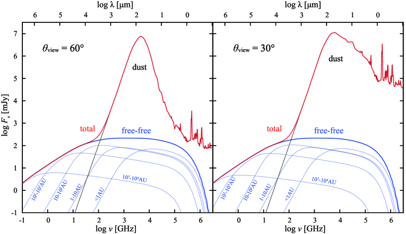
Figure 11.— SEDs for model A16 ($M_{c}=60\>M_{\odot}$, $\Sigma_{\rm cl}=1\>{\rm g\>cm^{-2}}$, and $m_{*}=16\>M_{\odot}$) at inclination angles of $60\arcdeg$ (left) and $30\arcdeg$ (right). Two emission components, free-free (thick blue) and thermal dust (thin black), are shown in each panel. The blue dotted lines show the contributions by the regions at $1,10,10^{2},10^{3}$ and $10^{4}\>{\rm AU}$ from the central star. A distance of $1\>{\rm kpc}$ is assumed for the flux normalizations.

3.2.1 Spectral Energy Distributions

For all SED calculations, a distance of $1\>{\rm kpc}$ and an aperture diameter of $20\arcsec$ (20,000 AU) are assumed. Figure 11 shows full SEDs including thermal dust and free-free emission for model A16 at viewing inclinations of $60\arcdeg$ and $30\arcdeg$ of the line of sight to the rotation/outflow axis. The flux from thermal dust emission was calculated by ZTH14. The free-free emission dominates over the thermal dust emission at radio frequencies of $\lesssim 100\>{\rm GHz}$, while the dust flux dominates at higher frequencies. We note that, at wavelengths shorter than $100\>{\rm\micron}$, we do not count the free-free emission in the total flux since we do not treat the dust extinction in the free-free radiative transfer calculation (eq. 7).

The infrared (IR) dust flux (at relatively short wavelengths) depends strongly on viewing angle. This is because the stellar radiation is absorbed by the dense disk and core envelope along directions close to the equatorial plane, and the re-emitted IR radiation, still suffering from high optical depths, escapes along the polar, low-density outflow cavity. Therefore, the observed flux is higher if the line of sight is passing through the outflow cavity (ZTH14). This process is known as the “flashlight effect,” which is also important for helping to overcome radiation pressure feedback (Nakano et al., 1995; Yorke & Bodenheimer, 1999; Krumholz et al., 2005, 2009; Kuiper et al., 2010, 2011).

On the other hand, the radio flux is almost independent of viewing angle since it typically experiences much smaller optical depths than the IR radiation. We can approximate the spectrum of free-free emission as being a power law in frequency, $F_{\nu,{\rm ff}}\propto\nu^{p}$, with spectral index $p$. From $3$ – $30\>{\rm GHz}$, the free-free flux from model A16 is fitted as $F_{\nu,{\rm ff}}=81(\nu/{\rm GHz})^{0.48}\>{\rm mJy}$. The spectral index of the free-free emission decreases from $p=0.9$ at 0.1 GHz to $0.2$ at 100 GHz. An index smaller than two indicates that the photoionized disk wind is only partially optically thick with respect to its free-free emission. The overall spectral index (including thermal dust emission) has a minimum of $0.45$ at $35\>{\rm GHz}$, and quickly increases at higher frequencies approaching the dust spectrum value of $p=3.3$. Figure 11 also indicates that the free-free flux at $\sim 0.1$ GHz is mostly emitted from $\sim 10^{3}$–$10^{4}$ AU scales, while that at $\sim 10$ GHz is mostly probing $\sim 10^{2}$–$10^{3}$ AU scales. Thus, the higher frequencies trace the structure of the inner wind.

Figure 12 shows SEDs for all models. The features of the free-free emission are similar to those discussed for model A16: the free-free fluxes at radio frequencies are almost independent of viewing angle, and are $\sim 20$ – $200\>{\rm mJy}$ with the spectral indices of $p\simeq 0.4$ – $0.7$ at $10\>{\rm GHz}$. These common features are caused by the fact that the outflows of all models have similar structures, i.e., the amount of gas and the density gradient. If the photoionized region is small, the free-free emission is not observable, as in, e.g., model Al08. Once the photoionized region breaks out, the free-free emission becomes bright, as in, e.g., model Al12. Since the flux of free-free emission depends on the density structure of the outflow, the mass of the outflow that is emitting free-free flux (within a given distance from the protostar) may be estimated from its free-free flux.

With our focus in this paper on radio wavelengths, we note again that we have not accounted for the free-free emission for the total flux at wavelengths less than $100\>\micron$. However, in some cases the free-free flux might make a significant contribution in this range: e.g., at wavelengths shorter than $10\micron$ of model C16 viewed at $60\arcdeg$. The potential importance of free-free emission at shorter wavelengths will be explored in a future paper.

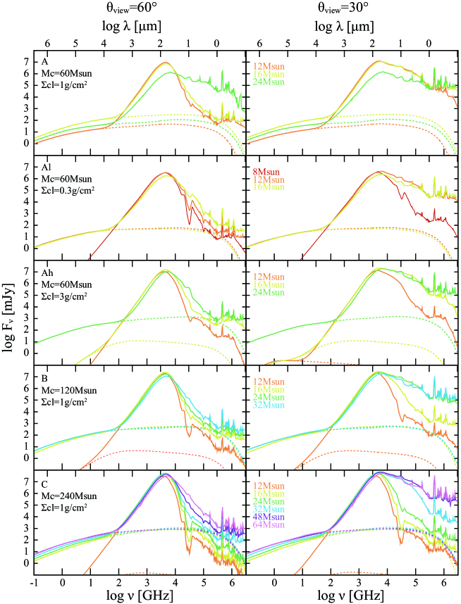
Figure 12.— The SEDs at inclination angles of $60\arcdeg$ (left) and $30\arcdeg$ (right) for model group A, Al, Ah, B and C (from top to bottom). The dotted lines show the free-free emission components.

3.2.2 Images

Next, we present images of the free-free emission. We show both resolved images and those after convolving with finite beam sizes of various telescopes. Detailed comparisons of models with individual sources are deferred to future papers in this series.

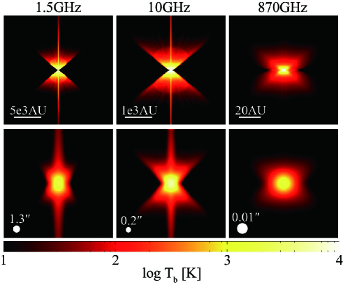
Figure 13.— Resolved (top) and convolved (bottom) images of model A16 ($M_{c}=60\>M_{\odot},\Sigma_{\rm cl}=1\>{\rm g\>cm^{-2}},{\rm~{}and~{}}m_{*}=16\>M_{\odot}$) at an inclination angle of $60\arcdeg$. The panels show the images at the frequencies of $1.5,~{}10,{\rm~{}and~{}}870\>{\rm GHz}$ from left to right. In the top panels, the box sizes are $20,000{\rm AU}\times 20,000{\rm AU}$, $4,000{\rm AU}\times 4,000{\rm AU}$, and $100{\rm AU}\times 100{\rm AU}$, respectively. In the bottom panels, the beam sizes (FWHM) at each frequency are indicated at the bottom-left corners ($1.3,~{}0.2,$ and $0.01\arcsec$). A distance of $1{\rm\>kpc}$ is assumed. In the convolved images of the bottom row, from left to right the brightness temperature of $T_{b}$ is equivalent to $3.1\mu{\rm Jy}(T_{b}/{\rm K}){\rm\>beam}^{-1}$, $3.3\mu{\rm Jy}(T_{b}/{\rm K}){\rm\>beam}^{-1}$ and $62\mu{\rm Jy}(T_{b}/{\rm K}){\rm\>beam}^{-1}$ at these given frequencies.

The top three panels of Figure 13 show the resolved free-free emission images of model A16 at the inclination of $60\arcdeg$ at three different frequencies, 1.5, 10, and 870 GHz. These frequencies correspond to the L and X bands of the Karl G. Jansky Very Large Array (J-VLA) and band 10 of the Atacama Large Millimeter/submillimeter Array (ALMA). Box sizes are $20,000\>{\rm AU}\times 20,000\>{\rm AU}$, $4,000\>{\rm AU}\times 4,000\>{\rm AU}$, and $100\>{\rm AU}\times 100\>{\rm AU}$, respectively. The apparent size of the free-free images is larger at lower frequencies since free-free absorption is stronger (eq. 8). The effective radius at which half of the total flux is emitted is $10^{-3}(\nu/10{\rm\>GHz})^{q}\>{\rm pc}\simeq 2\times 10^{2}(\nu/{10\rm\>GHz})^{q}\>{\rm AU}$, with $q\simeq-0.7$ for $1$–$100{\rm\>GHz}$. Thus these would typically be categorized as HC H II regions (see also §4.2). At 1.5 GHz and 10 GHz, the apparent shape is similar to an hour-glass shape with a jet, because the disk wind has a self-similar structure at the scale of $\gtrsim 1000\>{\rm AU}$. The surface brightness is high in the central wind region and at the jet axis where the density is high, and the maximum brightness temperature of $T_{b}\simeq 10^{4}\>{\rm K}$ indicates optically thick conditions. At the higher frequency of 870 GHz, the shape is now more rounded in the inner region. This is because of the accretion disk with radius of $\sim 100{\rm AU}$. The collimated on-axis jet is not seen, since it becomes optically thin at this frequency. For the total free-free flux in Figure 11, the innermost wind region dominates the on-axis jet since its area is bigger. However, the bright linear feature is still very interesting, since it is potentially related to observed radio jets (Gibb et al., 2003; Rodríguez et al., 2008; Guzmán et al., 2012, 2014).

The bottom three panels of Figure 13 show the free-free images convolved with the finite beam sizes of the telescopes at these frequencies. The full-width at half-maximum (FWHM) beam sizes are 1.3, 0.2, and 0.01 $\arcsec$ for 1.5, 10, and 870 GHz, respectively, i.e., the highest resolutions in the L and X bands of the J-VLA and in band 10 of ALMA. A distance of 1 kpc is assumed, and the point-spread function is approximated as a Gaussian function. The jet feature with high brightness temperature along the axis is diluted at 1.5 GHz and 8.4 GHz, since it is narrower than the beam size. However, the linear feature is still observable at the level of $T_{b}\lesssim 30{\rm\>K}$ or $100\mu{\rm Jy\>beam}^{-1}$ at both frequencies. The sensitivity with root-mean-square value of $\sim 10\mu{\rm Jy\>beam}^{-1}$ can be attained with an observing time of 1 hour and a bandwidth of 500 MHz by the J-VLA. The inner brightest region with $T_{b}\simeq 10^{4}{\rm\>K}$ is smaller than the beam size, and thus the highest brightness temperature decreases to $1600{\rm\>K}$ at 870 GHz. The dust emission cannot have a brightness temperature above the dust sublimation temperature of $1400\>{\rm K}$. Therefore, even though the total flux is dominated by dust emission at the frequencies $\gtrsim 100{\>\rm GHz}$ (Fig. 11), the free-free emission may be observable even at this high frequency. Since most massive protostars are at somewhat larger distances, this emission may need to be observed in more massive, denser sources.

Figure 14 shows resolved and convolved images at 10 GHz as the protostar evolves, viewed at inclination angles of $30\arcdeg$ and $60\arcdeg$ for all models. From the resolved images (top panels of Fig. 14), it can be seen that the outflow opening angle gradually increases, especially at the inclination of $60\arcdeg$, once the photoionized region is formed. When the line of sight passes through the outflow cavity ($\theta_{\rm view}<\theta_{\rm w,esc}$), like model A16 at $30\arcdeg$ inclination, then the image becomes elliptical rather than hourglass shaped. The outflow axis always exhibits a high brightness at this frequency. As stated above, the linear jet-like feature is observable at the level of $T_{b}\lesssim 30{\rm\>K}$ in the convolved image of model A16. In the case of higher-$\Sigma_{\rm cl}$ or $M_{c}$, the brightness temperature is higher since the outflow rate is higher. Thus the jet feature is observable even at $T_{b}\simeq 100{\rm\>K}$ in these models, such as models Ah24 and C32. The small spots in convolved images of models Ah16 and B12 are the sign of unresolved outflow-confined H II regions.

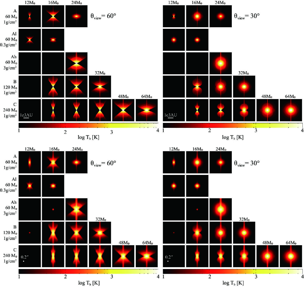
Figure 14.— Resolved (top) and convolved (bottom) images at 10 GHz of all models at inclination angles of line of sight of $60\arcdeg$ (left) and $30\arcdeg$ (right) to the outflow axis. The box size of top panels are $4,000{\rm\>AU}\times 4,000{\rm\>AU}$. The images in the bottom panels are convolved with a beam size of $0.2{\arcsec}$ and a distance of 1 kpc is assumed. Here, the brightness temperature of $T_{b}$ is equivalent to $3.3\mu{\rm Jy}(T_{b}/{\rm K}){\rm\>beam}^{-1}$.

3.3. Hydrogen recombination lines

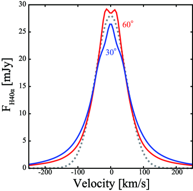
Figure 15.— H$40\alpha$ line profiles of model A16 viewed with inclination angles of $60\arcdeg$ (red solid line) and $30\arcdeg$ (blue solid line). The FWHM are $v_{\rm FWHM}=104,\>115\>{\rm km\>{s}^{-1}}$ at $60,\>30\arcdeg$ respectively. The gray dotted line shows a Gaussian distribution with $v_{\rm FWHM}=110\>{\rm km\>s^{-1}}$ and a peak flux of $28\>{\rm mJy}$. A distance of $1\>{\rm kpc}$ is assumed.

We perform radiative transfer of the H$40\alpha$ line to obtain simulated observations that probe the kinematics of the photoionized wind. Here, a distance of $1\>{\rm kpc}$ and aperture diameter of $20\arcsec$ (20,000 AU) are assumed.

Figure 15 shows profiles of H$40\alpha$ flux from model A16. The line profiles are very similar for the inclination angles of $60\arcdeg$ and $30\arcdeg$: the FWHM are $104{\rm~{}and~{}}115\>{\rm km\>s^{-1}}$, the peak fluxes are $29{\rm~{}and~{}}27\>{\rm mJy}$, the ratios of line flux to the free-free continuum flux are $0.16$ and $0.18$, respectively. Although we used a Gaussian line profile of $\phi_{\nu}$ at each position for the radiative transfer calculation (eq. 13), the obtained total spectrum has broader wings. This is because the disk wind has higher velocity components, $\gtrsim 500\>{\rm km\>s^{-1}}$, near the axis.

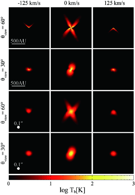
Figure 16.— H$40\alpha$ maps of model A16 at $-125,~{}0,{\rm~{}and~{}}125\>{\rm km\>s^{-1}}$ (from left to right). Top two rows show the resolved images viewed at inclination angles of $60\arcdeg$ (first row) and $30\arcdeg$ (second row). The box size is $1500\>{\rm AU}\times 1500\>{\rm AU}$. Bottom two rows show the convolved images viewed at inclination angles of $60\arcdeg$ (third row) and $30\arcdeg$ (fourth row). A beam size of 0.1$\arcsec$ and a distance of 1 kpc are assumed.

Figure 16 shows resolved and convolved maps of H$40\alpha$ of model A16 at three different velocities, $-125,~{}0,{\rm~{}and~{}}125\>{\rm km\>s^{-1}}$, at inclinations of $60\arcdeg$ and $30\arcdeg$. The map is convolved with a beam size of 0.1 ″ which is the highest resolution in band 3 of ALMA. For this ionized bipolar outflow, the blueshifted component appears on the north (upper) side and the redshifted component in south (lower) side. However, the $0{\rm\>km\>s^{-1}}$ maps are tilted slightly to northwest-southeast direction. This is due to the rotation of the outflow. Rotating outflows have been found around low-mass and intermediate-mass protostars (Klaassen et al., 2013; Codella et al., 2014), but not yet for high-mass objects. In resolved maps at an inclination of $60\arcdeg$, the line of sight is outside the cavity and thus the rim of the outflow is brightest. On the other hand, in resolved maps at an inclination of $30\arcdeg$, the line of sight passes through the cavity and the maps are elliptical illustrating the outflow cone. This difference becomes less clear in the convolved maps at $\pm 125{\rm\>km\>s^{-1}}$. However, it is still visible in the $0{\rm\>km\>s^{-1}}$ maps at the level of $T_{b}\simeq 10{\rm K}$. The sensitivity of $T_{b}=2{\rm K}$ could be attained with an observing time of 8 hours with a channel width of 6 MHz by ALMA. The effective spectral resolution is two times of the channel width which corresponds to 12 MHz or $36{\rm km\>s^{-1}}$ (the H40$\alpha$ HRL is at 99 GHz). We should mention that again a distance of 1 kpc is assumed here, and most massive protostars are typically at larger distances. Thus, this emission may need to be observed in more massive and denser sources.

3.4. Escape fraction of ionizing photons

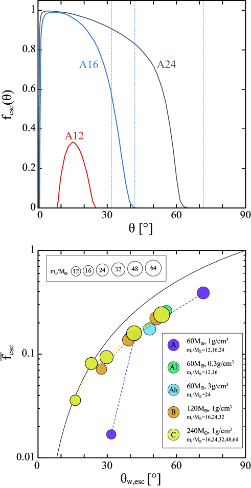
Figure 17.— Top: Escape fraction of ionizing photons to each polar angle for models A12, A16, and A24 (red, blue, and black solid lines, respectively). The dotted lines represent the opening angle of each model. Bottom: The total escape fraction of ionizing photon vs. the opening angle of the disk wind cavity. The circles show the models and the dotted lines represent their evolution (purple: model group A; green: Al; light blue: Ah; orange: B; and yellow: C). The size of each circle represents the protostellar mass. The solid line shows the covering fraction of the whole sky solid angle by the disk wind cavity, i.e., $1-\cos\theta_{\rm w,esc}$.

So far we presented results for the ionization of disk winds. Next, we consider the ionizing photons that escape along the outflow cavities created by these winds. Since the obtained ionized regions are unconfined in the radial direction, some fraction of ionizing photons escape and are expected to ionize the ambient clump gas. This ionization feedback, in addition to that of the disk wind protostellar outflows, may affect star formation around the forming massive star and will also lead to additional radio emission.

The top panel of Figure 17 shows the escape fraction of ionizing photons to each polar angle, $f_{\rm esc}(\theta)$, along with the opening angle of the disk wind cavity, $\theta_{\rm w,esc}$. In the case of model A12, the escape fraction is $0.35$ at its maximum value and almost zero for $\theta<10\arcdeg$ or $\theta>30\arcdeg$. This is because the ionized region is restricted to $10\arcdeg\lesssim\theta\lesssim 30\arcdeg$ (Fig. 4). As the ionized region expands in models A16 and A24, the angular range in which photons escape also expands and the maximum value of $f_{\rm esc}(\theta)$ reaches about unity. However, the escape fraction is still $<0.5$ in directions near the boundary of the core infall envelope (i.e., $\theta>\theta_{\rm w,esc}-10\arcdeg$: see also Fig. 5) or near the outflow axis ($\theta<5\arcdeg$: see also Fig. 6) due to strong attenuation in these higher density regions.

The bottom panel of Figure 17 shows the evolution of the outflow cavity opening angle, $\theta_{\rm w,esc}$, and the total escape fraction of ionizing photons, $\overline{f}_{\rm esc}$, for all model groups. It can be seen that the total escape fraction increases as the opening angle grows in every case. However, we note that, due to Hydrogen ionization and dust absorption, the total escape fraction is lower than the fraction of solid angle extended by the disk wind cavity. The maximum value of $\overline{f}_{\rm esc}$ in our models is $0.38$ with $\theta_{\rm w,esc}=72\arcdeg$, so more than half of ionizing photons do not escape from the system (including the directions blocked by the disk and infalling core envelope).

The total ionizing photon rate escaping from the protostellar core is $\overline{f}_{\rm esc}S_{\rm*,acc}$. Most of these photons will be able to ionize the ambient clump or larger-scale cloud gas, especially the gas in front of the head of the outflow bowshock. Our model does not explicitly include the structure of the outflow bowshock or the ambient clump gas. Thus, we do not study details of the geometry or kinematics of the ionized clump. Instead, as a simple first approximation, we use a Strömgren sphere analysis to make some simple estimations. In this case, the approximate size scale of the ionized region created by escaping photons is

$$R_{\rm St,cl}=\left(\frac{3\overline{f}_{\rm esc}S_{*,\rm acc}}{4\pi n_{\rm H,cl}^{2}\alpha_{\rm B}}\right)^{1/3},$$ (16)

where $n_{\rm H,cl}$ is the density of the ambient clump, and $\alpha_{\rm B}=\alpha_{\rm A}-\alpha_{1}$ is the case B recombination rate (this estimate ignores absorption of photons by dust). The mean clump density is given by $n_{\rm H,cl}=2.0\times 10^{5}({\Sigma_{\rm cl}}/{1\>{{\rm g\>cm^{-2}}}})^{3/2}(M_{\rm cl}/4000\>M_{\odot})^{-1/2}{\>\rm cm^{-3}}$. The recombination rate, $\alpha_{\rm B}$, is a function of temperature, which is calculated from the stellar spectrum and the clump density (§2.2.3). The free-free emission is evaluated by solving equation (7) assuming spherical geometry. The FWHM of the velocity distribution of the ionized clump gas, which will be used as part of the diagnostic process to classify H II regions (§4), is estimated simply from thermal broadening, $v_{\rm FWHM,cl}=\sqrt{8\ln{2}}\sigma_{v}$. This estimation gives the minimum value of the line width, since the clump gas could also be disturbed by outflows and additional turbulent motions that broaden the line profile.

We note some caveats of this Strömgren sphere approximation for ambient clump ionization. First, the geometry of the ionized region is likely to be affected by the outflow cavity, leading to deviations from a simple sphere. Second, the ambient clump density is expected to be inhomogeneous, which can lead to various effects, including enhanced effective densities at ionization fronts that can lead to smaller H II region sizes (e.g., Tan & McKee, 2004). Thus, the free-free flux evaluated by the Strömgren sphere analysis is only expected to be a very crude approximation. If the ambient clump region is optically thin, its total free-free flux from the ionized region is just proportional to the total escaping photon rate, $\overline{f}_{\rm esc}S_{\rm*,acc}$, regardless of its shape or density. However, if the ionized region is optically thick, the free-free flux is smaller than the optically thin limit by the factor of its mean optical depth. Therefore, the error in the free-free flux would be small if the ionized clump region is optically thin.

4. Discussion

4.1. Outflow-confined H II regions and their break out

Here we summarize the evolution of ionized outflows. Note, the increase of ionizing flux in the Kelvin-Helmholz contraction phase is very rapid (Fig. 2) and our numerical results have only been carried out with relatively coarse sampling across the evolutionary sequence. However, we can still present a description of the following evolutionary sequence. At the first stage, when the ionizing flux is small, the MHD-driven outflow is the first barrier to the propagation of ionizing photons, except in the very narrow range of directions within the inner disk wind cavity. The H II region is confined in a very thin layer of the inner outflow wall, e.g., model Ah16 in Figure 8. As the ionizing flux increases, the H II region extends to greater distance from the protostar. At a critical ionizing flux, the H II region breaks out at a middle latitude (see model A12 in Fig 4). At the lower latitude, the density is higher than that in the middle latitude since it is closer to the launching zone of the disk wind. On the other hand, the density gradient at the higher latitude is flatter than that at the middle latitude due to the collimated structure of the wind. Therefore, the H II region breakout starts from $\theta\simeq\theta_{\rm w,esc}/2$. The critical ionizing flux for the radial breakout depends on the detailed structure of outflow, i.e., mass loss rate, opening angle and velocity structure. From a qualitative standpoint, the mass loss rate is roughly proportional to the mass accretion rate, and thus the critical ionizing flux for the breakout is higher for higher-$\Sigma_{\rm cl}$ cases. The breakout does not occur at $8\>M_{\odot}$ even in the low-$\Sigma_{\rm cl}$ case of model Al08. The typical flux for breakout is $10^{46}$–$10^{47}\>{\rm s}^{-1}$ in our numerical calculations, which is as high as the flux from the ZAMS at about $10$–$15\>M_{\odot}$. All models in this work reach $20\>M_{\odot}$ at the final stage, however, it should be noted that there are almost as many stars between $8$ and $10\>M_{\odot}$ as above $20\>M_{\odot}$. In the formation of such stars with $\lesssim 10\>M_{\odot}$, the H II region is confined during the main accretion phase and breakout occurs only towards the end of accretion when the outflow rate also decreases.

After first breakout at $\theta_{\rm w,esc}/2$, the photoionized region extends in polar angle. To ionize almost the entire outflow, the ionizing flux needs to increase by about one order of magnitude from the first breakout ionizing flux. This takes only $10^{3}$–$10^{4}{\>\rm yr}$ since the ionizing flux increases rapidly in the KH contraction phase. Once the entire outflow is ionized, the expansion in polar angle of the H II region slows down matching the increase of the outflow cavity opening angle, which has a timescale similar to the accretion time, i.e., $m_{*}/\dot{m}_{*}\sim 10^{4}$–$10^{5}{\>\rm yr}$.

Our model of photoionized disk winds may also help to explain the short timescale variability that is seen in some UC/HC H II regions (Franco-Hernández & Rodríguez, 2004; Rodríguez et al., 2007; Galván-Madrid et al., 2008) and which has also been modeled in the radiative hydrodynamical simulations of Peters et al. (2010). Fluctuations in the accretion rate would also lead to changes in the outflow massloss rate, which would change the density and thus the extent of the photoionized region. Changes could happen on outflow crossing timescales, i.e., as short as $\sim 0.01$ pc / $1000\>{\rm km\>s}^{-1}\simeq 10$ yr.

Our model makes prediction for the spectral and the size indices, i.e., $p$ and $q$, of the free-free emission. The free-free emission spectral index at 10 GHz is about $p=0.4$–$0.7$ (see §3.2.1), which indicates that the outflow is partially optically thick. The apparent size of the observed free-free emission (see §3.2.2) is as small as $\sim 10^{-3}{\rm\>pc}$ at 10 GHz and smaller at higher frequencies, scaling with size as $r\propto\nu^{q}$, with the index of $q\simeq-0.7$, even though the ionized region is larger than the core scale of $0.1\>{\rm\>pc}$ after breakout. These frequency dependences are related to the density structure of the ionized outflow. A simplest analytical structure is a spherical wind with constant velocity, i.e., $n_{\rm H}=\dot{m}_{w}/(4\pi r^{2}v_{w})$ where $\dot{m}_{w}$ and $v_{w}$ are the wind mass loss rate and velocity (Panagia & Felli, 1975). Since the opacity for the free-free emission at radio frequencies is approximatly $\kappa_{\nu,\rm ff}\propto n_{\rm H}^{2}\nu^{-2.1}$ if the gas is isothermal, the optical depth rapidly decreases as $r^{-3}$. Therefore, the outer region becomes optically thin and has less contribution to the total free-free flux even though the ionized gas extends to larger scales. In this spherical model, the radius of the optically thick region scales as $r_{\tau_{\nu}=1}\propto\nu^{-0.7}$, and thus the total free-free flux, which is proportional to the flux from the optically thick region, is $F_{\nu,\rm ff}\propto B_{\nu}r_{\tau_{\nu}=1}^{2}\propto\nu^{0.6}$. Additionally, as shown by Reynolds (1986), even with a bipolar jet geometry, the set of indices will be similar to the simple spherical wind if the jet is conical (constant aperture angle), of constant velocity and ionization fraction, and is isothermal. Thus the departure from the indices of $(p,\>q)=(0.6,\>-0.7)$ is related to acceleration, collimation, thermal structure, or variation of ionization fraction (Reynolds, 1986; Guzmán et al., 2014). Our wind model is more complex compared to the spherical wind or the conical jet, however the fundamental physics is the same and thus the values of its spectral and size indices are similar.

4.2. Comparison with observed radio sources around massive protostars

Here, we compare general properties of our model with observed radio sources around massive protostars and show that the features of our theoretical models are similar to those of observed radio winds and jets.

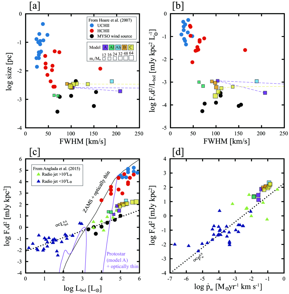
Figure 18.— Properties of theoretical outflow-confined H II region models compared with observed radio sources around protostars. The observational data are adopted from Hoare et al. (2007), Hoare & Franco (2007) (filled circles in panels (a), (b), and (c)), and from Anglada et al. (2015) (filled triangles in panels (b) and (c)). In all panels, the theoretical models are shown by square symbols with sizes indicating the stellar mass $m_{*}$ (purple: model group A, green: Al, light blue: Ah, orange: B, and yellow: C). The dash lines represent evolution within the model groups. (a): Size versus line width. Observed objects are shown by circles (blue: UC H II regions, red: HC H II regions, and black: MYSO wind sources). The sizes for the theoretical models (which vary with frequency) and the observed sources have both been evaluated at $8\>{\rm GHz}$. (b): The ratio of radio and bolometric luminosities versus line width. Symbols are same as the panel (a). The radio luminosity for the theoretical models, which varies with frequency, and the observed sources have been evaluated at $8\>{\rm GHz}$. (c): Radio luminosity versus bolometric luminosity. Triangles show observed radio jets (light green: high-luminosity, and blue: low-luminosity sources). The radio luminosities of the theoretical models are evaluated at $8\>{\rm GHz}$, and the observational data are at $5$ or $8\>{\rm GHz}$. The dotted line shows the fitting by Anglada et al. (2015): $F_{\nu}d^{2}/{\rm mJy\>kpc^{2}}=8\times 10^{-3}\left(L_{\rm bol}/L_{\odot}\right)^{0.6}$. This relation is based on observed radio jets over a wide bolometric luminosity range of $1$–$10^{5}L_{\odot}$. The solid line shows the estimated radio flux from an optically thin H II region based on the ionizing luminosities of ZAMS stellar models by Thompson (1984). The purple line shows the estimated radio flux from an optically thin H II region based on the ionizing luminosities of the protostar of model group A. (d): Radio luminosity versus outflow momentum rate. The dotted line shows the fitting by Anglada et al. (2015): $F_{\nu}d^{2}/{\rm mJy\>kpc^{2}}=190\left({\dot{p}_{w}}/{M_{\odot}\>{\rm yr}^{-1}{\rm\>km\>s^{-1}}}\right)^{0.9}$. The square and triangle symbols and the purple line are same as in panel (c). The momentum rate of our model $\dot{p}_{w}$ is obtained from the evolution calculation by ZTH14 rather than from estimation by a synthetic observation. Properties of the theoretical models of outflow-confined H II regions are broadly consistent with those of the high luminosity end of the observed radio wind/jet sources.

Figure 18 shows the properties of size, line width, radio and bolometric luminosities, and outflow momentum rate of our models and of observed radio sources. For our models, size and free-free luminosity are measured at $8\>{\rm GHz}$ and line width is evaluated from H$40\alpha$ assuming an inclination angle of $60\arcdeg$. The size is evaluated by the diameter at which half of the total radio flux of the system is emitted. As we have seen, the inclination angle does not affect these properties significantly at radio frequencies. Note, the outflow momentum rate, $\dot{p}_{w}$, of our model shown in Figure 18 is obtained from the protostellar evolution calculation of ZTH14 rather than from an estimation via a synthetic observation.

In panel (a) of Figure 18, we show how Hoare et al. (2007) distinguished objects into three categories based on size and line width: UC H II regions are $\sim 0.1{\rm\>pc}$ and $<40\>{\rm\>km\>s^{-1}}$, HC H II regions are $<0.05{\rm\>pc}$ and $>40\>{\rm\>km\>s^{-1}}$, and massive young stellar object (MYSO) wind sources are $<0.005{\rm\>pc}$ and $>70{\rm\>km\>s^{-1}}$. It should be noted that this classification of the radio sources is somewhat arbitrary. For example, Kurtz (2002, 2005) defined UC H II regions as having diameters $\leq 0.1{\rm\>pc}$ and HC H II regions as $\leq 0.01{\rm\>pc}$ with emission measures $\geq 10^{8}{\rm\>pc\>cm^{-6}}$. Tan et al. (2014) adopts a simpler definition only based on the above sizes. When we refer to data from Hoare et al. (2007) and Hoare & Franco (2007), we follow Hoare et al.’s classification. The line width of UC and HC H II regions are derived from radio HRLs, while those of wind sources are from IR HRLs. The wind sources (BN, W33A, S140 IRS 1, NGC 2024 IRS 2, GL 989 and GL 490 are plotted here) are the smallest and fastest objects. Comparing in those plots, our models reproduce the properties of wind sources quantitatively, with sizes of $\sim 10^{-3}\>{\rm pc}$ and line widths of $\sim 100{\rm\>km\>s^{-1}}$. Two of our models have broader line widths than $250{\rm\>km\>s^{-1}}$ ($718{\rm\>km\>s^{-1}}$ for A12 and $429{\rm\>km\>s^{-1}}$ for C16). These two models are at the beginning of H II region expansion, and the ionized region is confined only near the axis where the wind velocity is highest. Thus, their line width is exceptionally broad.

The difference between UC/HC H II regions and MYSO wind sources is more clearly seen in the ratio of radio and bolometric luminosities in panel (b) of Figure 18. UC/HC H II regions are more radio-loud than MYSO wind sources by two orders of magnitude or more. Even though the average radio to bolometric luminosity ratio of our models are about one order of magnitude higher than those of MYSO wind sources, there is still overlap given their dispersions.

Anglada et al. (2015) found two empirical correlations related to the radio luminosity of observed radio jets: one is a correlation with bolometric luminosity; the other is with outflow momentum rate:

$$\frac{F_{\nu}d^{2}}{{\rm\>mJy\>kpc^{2}}} = 8\times 10^{-3}\left(\frac{L_{\rm bol}}{L_{\odot}}\right)^{0.6};$$ (17)

$$\frac{F_{\nu}d^{2}}{{\rm\>mJy\>kpc^{2}}} = 190\left(\frac{\dot{p}_{w}}{M_{\odot}\>{\rm yr}^{-1}{\rm\>km\>s^{-1}}}\right)^{0.9}.$$ (18)

Interestingly, those two correlations are consistent over a wide bolometric luminosity range of $\sim 1\>L_{\odot}$ to $\sim 10^{5}\>L_{\odot}$ (dotted lines in panels (c) and (d) of Fig. 18). MYSO wind sources from Hoare & Franco (2007) (black circles) also fall on the first correlation. The solid line in panel (b) is the expected radio luminosity in the optically thin limit using the ionizing photon rate of ZAMS models by Thompson (1984), which represents the maximum radio luminosity from photoionized gas. At $L_{\rm bol}\lesssim 10^{3}\>L_{\odot}$, however, there are radio jets that exceed this maximum value (Anglada et al., 1992). It has been suggested that the single power law correlations of equations (17) and (18) indicates a common nature of (ionized) outflows from low-mass and high-mass protostars (Rodríguez et al., 1989b; Anglada, 1995). Since the photoionization properties differ greatly from low-mass to high-mass stars, this might imply that a different mechanism, i.e., shock ionization, is responsible for the observed radio emission along these correlations. However, we find that the radio luminosities of our model agree reasonably well with both the correlations of eqs. (17) and (18), even though they are photoionized structures. We predict that there should be a transition to photoionization-dominated winds for massive protostars, but that in this regime the radio/bolometric luminosities and the outflow momentum rate may not differ too much from this empirical relation. The systematic differences of our models are towards somewhat higher values of radio luminosities by factors of 1.5–13. This may be a signature of the initial stage of photoionization leading to enhanced radio fluxes. Note, our models tend to be more massive than the observed sources, so more data in this range is needed.

If the photoionized region is optically thin, the free-free emission is simply proportional to the ionizing photon flux rate (Hummer & Seaton, 1963). However, our model indicates much lower free-free flux than the optically thin limit (panel (c) in Fig. 18). First, this is because more than half of the emitted ionizing photons are absorbed at the innermost region of $r\ll 1000{\rm AU}$. This region is optically thick for the radio free-free emission, and thus the absorption there does not contribute to the total free-free flux. In the case of model A16, $78\%$ of photons are absorbed inside $r\leq 100{\rm AU}$. Second, most of the rest of the photons, ${\bar{f}}_{\rm esc}$, escape from the system. Those escaping photons do not induce free-free flux from the core scale, but contribute to the flux from the ambient clump gas, which is discussed below (§4.3). The final reason is that the photoevaporation flow has so far not been included in our model. If the ionizing photon rate is high enough to ionize the disk and envelope surfaces, e.g., in the case of model A24, the outflow rate of ionized gas increases and the free-free flux should be enhanced. While the first and second reasons are physical, the last one is due to the incompleteness of our model. We will address photoevaporation and its feedback effects in a subsequent paper.

Our ionized outflow models typically have spectral indices with $p=0.4$–$0.7$ (Fig. 12), and size index with frequency of $q\simeq-0.7$ from free-free emission at 10 GHz (Fig. 13). As discussed above, those indices are related to the density gradient of the outflow. The indices obtained by our calculations are consistent with some observed radio jets, such as MWC 349 ($p=0.67\pm 0.03$ and $q=-0.74\pm 0.03$, Tafoya et al., 2004) and W75N(B) ($p=0.61\pm 0.03$ and $q=-0.7\pm 0.03$, Carrasco-González et al., 2015). G345.4938+01.4677, however, has the slightly steeper indices of $p=0.92\pm 0.01$ and $q=-1.1^{+0.5}_{-0.4}$ than our model, which may be interpreted as being due to a stronger degree of collimation and acceleration (Guzmán et al., 2014, Guzmán et al., in prep.).

We should notice that, even though our theoretical model has similar properties to those of the observed radio jets, there is still a lack of some physical processes in our model. The velocity of some jets is estimated to be as high as $500{\rm\>km\>s^{-1}}$ from the proper motion of associated lobes along the axes, e.g., HH 80-81 (Martí et al., 1998, 1995; Masqué et al., 2015) and Cep A HW 2 (Curiel et al., 2006). Similar to these sources, our wind models have high radio brightnesses and high velocities of $\gtrsim 300\>{\rm\>km\>s^{-1}}$ near the axes (Figs. 1, 7, etc.). However, unlike our model, some of lobes are found to have the radio emission with negative spectral indices, such as Serpens (Rodríguez et al., 1989a), HH 80-81 (Martí et al., 1993), Ceph A HW 2 (Garay et al., 1996), W3(OH) (Wilner et al., 1999), and IRAS 16547-4247 (Rodríguez et al., 2005). These negative spectral indices can be interpreted as due to nonthermal synchrotron emission induced by strong shocks with the ambient gas (Araudo et al., 2007), and this has been confirmed by the detection of linearly polarized emission in HH 80-81 (Carrasco-González et al., 2010). Additionally, our simple axisymmetric model has not accounted for the possibility of outflow axis precession, which is apparent in IRAS16547-4247 (Rodríguez et al., 2008). Although the current number of sources with these features is relatively small, inclusion of such additional physics in our theoretical models, i.e., shock ionization and outflow axis precession, are likely to be needed for a complete understanding of jet properties in massive star formation. Such analysis is also deferred to a future paper.

As we have seen, the properties of our models are consistent with the so-called “MYSO wind sources” in Hoare et al. (2007) and Hoare & Franco (2007), and “radio jets” with high bolometric luminosity in Anglada et al. (2015). In general, the main difference of “winds” and “jets” is the shape, i.e., winds have relatively wide opening angles and jets are more collimated bipolar outflows. This difference could be related to evolutionary stage (see also Fig. 14). To clarify our view of the evolutionary sequence of massive star formation and its outflow launching mechanism, further study is needed utilizing multi-wavelength observations to be compared with theoretical models.

4.3. Ionization of ambient clump gas by escaping photons

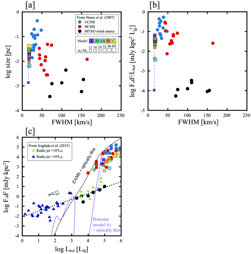
Figure 19.— Same as panels (a), (b) and (c) of Figure 18, except theoretical models now account for the escape of ionizing photons from the disk wind cavity.

Finally, we comment on the ionization of the ambient clump. Tens of percent of the total ionizing photon output escape along the outflow cavity (Fig. 17). These photons are likely to ionize the ambient clump which would lead to enhanced radio luminosity. We estimate features of these extended ionized regions, as described in §3.4. Figure 19 shows the comparison of our ionized clump models and observed sources (the observational data are the same as in Fig. 18). The Strömgren-based models of ionized ambient clumps typically have the size of $\sim 10^{-2}\>{\rm pc}$ and line widths of $\sim 20{\rm\>km\>s^{-1}}$, and large radio luminosities of $\gtrsim 10^{2}\>{\rm mJy\>kpc^{2}}$, which are larger in size, narrower in line width, and more radio loud than the ionized outflow models. These features are roughly consistent with observed UC/HC H II regions, except the line widths are broader in the observed systems. However, this difference is not surprising as the theoretical models include only thermal broadening and so give minimum widths.

We conclude that some UC/HC H II regions may be formed by the escaping photons from massive protostars with radio jets or winds. In this study, the ionized clump features are evaluated based on the simple Strömgren analysis (§3.4). For more detailed analysis, planned for future work, one needs to model more accurately the structure and kinematics of ambient clump gas, including its perturbation by the outflow, to better understand the connection of radio winds/jets and UC/HC H II regions.

5. Summary

We have studied the structure, evolution and observational properties of photoionized disk wind outflows that are expected to be associated with massive protostars forming by Core Accretion. Specifically, we have followed the quantitative properties of the Turbulent Core Accretion Model of McKee & Tan (2003) and follow-up protostellar evolution, disk wind and IR continuum radiative transfer models of Zhang & Tan (2011) and Zhang et al. (2013, 2014).

We calculated the transfer of ionizing photons and obtained the photoionized structure. The disk wind starts to be ionized when the stellar mass reaches about $10$ – $20\>M_{\odot}$, depending on the properties of the initial cloud core, due to the stellar temperature increase resulting from Kelvin-Helmholz contraction. At this moment, the photoionized region is confined to zenith angles of about $10$ – $30\arcdeg$, while the high density regions near the outflow axis and equatorial plane remain neutral. On the other hand, in the radial direction, the photoionized region is unconfined, since the density gradient of the disk wind is steep. The disk wind is almost entirely ionized in about $10^{3}$ – $10^{4}{\rm yr}$, and the photoionized region extends as the outflow opening angle increases. The outer disk surface is not ionized even though the diffuse radiation has been considered. This is because of the shielding effects of the inner disk and the disk wind.

Using the obtained photoionized structures, we calculated radiative transfer of free-free continuum and Hydrogen recombination line emission. The free-free emission exceeds dust emission at the radio frequencies lower than $100\>{\rm GHz}$ once the ionized region is formed. While shorter wavelength infrared flux from dust emission can depend on inclination of viewing angle, the radio flux from free-free emission is almost independent of inclination and its typical flux density is $\sim(20\>$–$\>200)\times(\nu/10{\rm GHz})^{p}{\rm\>mJy}$ at a distance of 1 kpc with a spectral index $p\simeq 0.4\>$–$\>0.7$ The apparent size depends on frequency as approximately $500(\nu/10{\rm GHz})^{-0.7}\>{\rm AU}$. The profile of ${\rm H40\alpha}$ has a FWHM of $\sim 100\>{\rm\>km\>s^{-1}}$ with broad wings. These properties of our model are similar to those of observed radio winds and jets from massive protostars. Detailed comparison with individual sources is deferred to future papers in this series.

References

- Anglada et al. (1992) Anglada, G., Rodríguez, L. F., Canto, J., Estalella, R., & Torrelles, J. M. 1992, ApJ, 395, 494
- Anglada (1995) Anglada, G. 1995, Revista Mexicana de Astronomia y Astrofisica Conference Series, 1, 67
- Anglada et al. (2015) Anglada, G., Rodríguez, L. F., & Carrasco-Gonzalez, C. 2015, Advancing Astrophysics with the Square Kilometre Array (AASKA14), 121
- Araudo et al. (2007) Araudo, A. T., Romero, G. E., Bosch-Ramon, V., & Paredes, J. M. 2007, A&A, 476, 1289
- Báez-Rubio et al. (2013) Báez-Rubio, A., Martín-Pintado, J., Thum, C., & Planesas, P. 2013, A&A, 553, AA45
- Beuther et al. (2002) Beuther, H., Schilke, P., Sridharan, T. K., et al. 2002, A&A, 383, 892
- Blandford & Payne (1982) Blandford, R. D., & Payne, D. G. 1982, MNRAS, 199, 883
- Bunn et al. (1995) Bunn, J. C., Hoare, M. G., & Drew, J. E. 1995, MNRAS, 272, 346
- Butler & Tan (2012) Butler, M. J., & Tan, J. C. 2012, ApJ, 754, 5
- Butler et al. (2014) Butler, M. J., Tan, J. C., & Kainulainen, J. 2014, ApJ, 782, LL30
- Carrasco-González et al. (2010) Carrasco-González, C., Rodríguez, L. F., Anglada, G., et al. 2010, Science, 330, 1209
- Carrasco-González et al. (2015) Carrasco-González, C., Torrelles, J. M., Cantó, J., et al. 2015, Science, 348, 114
- Castelli & Kurucz (2004) Castelli, F., & Kurucz, R. L. 2004, IAU Symp. No 210, Modelling of Stellar Atmospheres, eds. N. Piskunov et al. 2003, poster A20, arXiv:astro-ph/0405087
- Codella et al. (2014) Codella, C., Cabrit, S., Gueth, F., et al. 2014, A&A, 568, L5
- Curiel et al. (2006) Curiel, S., Ho, P. T. P., Patel, N. A., et al. 2006, ApJ, 638, 878
- Dale et al. (2005) Dale, J. E., Bonnell, I. A., Clarke, C. J., & Bate, M. R. 2005, MNRAS, 358, 291
- Davies et al. (2011) Davies, B., Hoare, M. G., Lumsden, S. L., et al. 2011, MNRAS, 416, 972
- Draine (2011) Draine, B. T. 2011, Physics of the Interstellar and Intergalactic Medium by Bruce T. Draine. Princeton University Press, 2011. ISBN: 978-0-691-12214-4
- Dupree & Goldberg (1970) Dupree, A. K., & Goldberg, L. 1970, ARA&A, 8, 231
- Ferland et al. (2013) Ferland, G. J., Porter, R. L., van Hoof, P. A. M., et al. 2013, RMxAA, 49, 137
- Figer (2005) Figer, D. F. 2005, Nature, 434, 192
- Franco-Hernández & Rodríguez (2004) Franco-Hernández, R., & Rodríguez, L. F. 2004, ApJ, 604, L105
- Galván-Madrid et al. (2008) Galván-Madrid, R., Rodríguez, L. F., Ho, P. T. P., & Keto, E. 2008, ApJ, 674, L33
- Garay et al. (2007) Garay, G., Mardones, D., Bronfman, L., et al. 2007, A&A, 463, 217
- Garay et al. (1996) Garay, G., Ramirez, S., Rodriguez, L. F., Curiel, S., & Torrelles, J. M. 1996, ApJ, 459, 193
- Gibb et al. (2003) Gibb, A. G., Hoare, M. G., Little, L. T., & Wright, M. C. H. 2003, MNRAS, 339, 101
- Goodman et al. (1993) Goodman, A. A., Benson, P. J., Fuller, G. A., & Myers, P. C. 1993, ApJ, 406, 528
- Guzmán et al. (2012) Guzmán, A. E., Garay, G., Brooks, K. J., & Voronkov, M. A. 2012, ApJ, 753, 51
- Guzmán et al. (2014) Guzmán, A. E., Garay, G., Rodríguez, L. F., et al. 2014, ApJ, 796, 117
- Hoare et al. (2007) Hoare, M. G., Kurtz, S. E., Lizano, S., Keto, E., & Hofner, P. 2007, Protostars and Planets V, 181
- Hoare & Franco (2007) Hoare, M. G., & Franco, J. 2007, A Volume Honouring John Dyson, Edited by T.W. Hartquist, J. M. Pittard, and S. A. E. G. Falle. Series: Astrophysics and Space Science Proceedings. Springer Dordrecht, 2007, p.61, arXiv:0711.4912
- Hollenbach et al. (1994) Hollenbach, D., Johnstone, D., Lizano, S., & Shu, F. 1994, ApJ, 428, 654
- Hosokawa & Omukai (2009) Hosokawa, T., & Omukai, K. 2009, ApJ, 703, 1810
- Hosokawa et al. (2010) Hosokawa, T., Yorke, H. W., & Omukai, K. 2010, ApJ, 721, 478
- Hosokawa et al. (2011) Hosokawa, T., Omukai, K., Yoshida, N., & Yorke, H. W. 2011, Science, 334, 1250
- Hummer & Seaton (1963) Hummer, D. G., & Seaton, M. J. 1963, MNRAS, 125, 437
- Keto (2007) Keto, E. 2007, ApJ, 666, 976
- Klaassen et al. (2013) Klaassen, P. D., Juhasz, A., Mathews, G. S., et al. 2013, A&A, 555, A73
- Königl & Pudritz (2000) Königl, A., & Pudritz, R. E. 2000, Protostars and Planets IV, 759
- Kratter et al. (2008) Kratter, K. M., Matzner, C. D., & Krumholz, M. R. 2008, ApJ, 681, 375
- Krumholz et al. (2009) Krumholz, M. R., Klein, R. I., McKee, C. F., Offner, S. S. R., & Cunningham, A. J. 2009, Science, 323, 754
- Krumholz et al. (2005) Krumholz, M. R., McKee, C. F., & Klein, R. I. 2005, ApJ, 618, L33
- Krumholz et al. (2007) Krumholz, M. R., Stone, J. M., & Gardiner, T. A. 2007, ApJ, 671, 518
- Kuiper et al. (2010) Kuiper, R., Klahr, H., Beuther, H., & Henning, T. 2010, ApJ, 722, 1556
- Kuiper et al. (2011) Kuiper, R., Klahr, H., Beuther, H., & Henning, T. 2011, ApJ, 732, 20
- Kurtz (2002) Kurtz, S. 2002, Hot Star Workshop III: The Earliest Phases of Massive Star Birth, 267, 81
- Kurtz (2005) Kurtz, S. 2005, Massive Star Birth: A Crossroads of Astrophysics, 227, 111
- Lanz & Hubeny (2007) Lanz, T., & Hubeny, I. 2007, ApJS, 169, 83
- Li et al. (2012) Li, J., Wang, J., Gu, Q., Zhang, Z.-y., & Zheng, X. 2012, ApJ, 745, 47
- López-Sepulcre et al. (2009) López-Sepulcre, A., Codella, C., Cesaroni, R., Marcelino, N., & Walmsley, C. M. 2009, A&A, 499, 811
- Martí et al. (1993) Martí, J., Rodríguez, L. F., & Reipurth, B. 1993, ApJ, 416, 208
- Martí et al. (1995) Martí, J., Rodríguez, & Reipurth, B. 1995, ApJ, 449, 184
- Martí et al. (1998) Martí, J., Rodríguez, L. F., & Reipurth, B. 1998, ApJ, 502, 337
- Martins & Plez (2006) Martins, F., & Plez, B. 2006, A&A, 457, 637
- Masqué et al. (2015) Masqué, J. M., Rodríguez, L. F., Araudo, A., et al. 2015, ApJ, in press (arXiv:1510.01769)
- Matzner & McKee (2000) Matzner, C. D., & McKee, C. F. 2000, ApJ, 545, 364
- McKee & Tan (2003) McKee, C. F., & Tan, J. C. 2003, ApJ, 585, 850 (MT03)
- McKee & Tan (2008) McKee, C. F., & Tan, J. C. 2008, ApJ, 681, 771
- McLaughlin & Pudritz (1997) McLaughlin, D. E., & Pudritz, R. E. 1997, ApJ, 476, 750
- Meynet et al. (2010) Meynet, G., Georgy, C., Revaz, Y., et al. 2010, Revista Mexicana de Astronomia y Astrofisica Conference Series, 38, 113
- Nakano et al. (1995) Nakano, T., Hasegawa, T., & Norman, C. 1995, ApJ, 450, 183
- Nisini et al. (1994) Nisini, B., Smith, H. A., Fischer, J., & Geballe, T. R. 1994, A&A, 290, 463
- Palau et al. (2013) Palau, A., Fuente, A., Girart, J. M., et al. 2013, ApJ, 762, 120
- Panagia & Felli (1975) Panagia, N., & Felli, M. 1975, A&A, 39, 1
- Peters et al. (2010) Peters, T., Klessen, R. S., Mac Low, M.-M., & Banerjee, R. 2010, ApJ, 725, 134
- Peters et al. (2011) Peters, T., Banerjee, R., Klessen, R. S., & Mac Low, M.-M. 2011, ApJ, 729, 72
- Reynolds (1986) Reynolds, S. P. 1986, ApJ, 304, 713
- Richling & Yorke (1997) Richling, S., & Yorke, H. W. 1997, A&A, 327, 317
- Rodríguez et al. (1989a) Rodríguez, L. F., Curiel, S., Moran, J. M., et al. 1989a, ApJ, 346, L85
- Rodríguez et al. (2005) Rodríguez, L. F., Garay, G., Brooks, K. J., & Mardones, D. 2005, ApJ, 626, 953
- Rodríguez et al. (2007) Rodríguez, L. F., Gómez, Y., & Tafoya, D. 2007, ApJ, 663, 1083
- Rodríguez et al. (2008) Rodríguez, L. F., Moran, J. M., Franco-Hernández, R., et al. 2008, AJ, 135, 2370
- Rodríguez et al. (1989b) Rodríguez, L. F., Myers, P. C., Cruz-Gonzalez, I., & Terebey, S. 1989b, ApJ, 347, 461
- Salem & Brocklehurst (1979) Salem, M., & Brocklehurst, M. 1979, ApJS, 39, 633
- Shakura & Sunyaev (1973) Shakura, N. I., & Sunyaev, R. A. 1973, A&A, 24, 337
- Shu (1977) Shu, F. H. 1977, ApJ, 214, 488
- Stone et al. (1992) Stone, J. M., Mihalas, D., & Norman, M. L. 1992, ApJS, 80, 819
- Strelnitski et al. (1996) Strelnitski, V. S., Ponomarev, V. O., & Smith, H. A. 1996, ApJ, 470, 1118
- Tafoya et al. (2004) Tafoya, D., Gómez, Y., & Rodríguez, L. F. 2004, ApJ, 610, 827
- Tan & McKee (2003) Tan, J. C., & McKee, C. F. 2003, IAU Symposium 221, Star Formation at High Angular Resolution, Eds. M. Burton, R. Jayawardhana, & T. Bourke, arXiv:astro-ph/0309139
- Tan & McKee (2004) Tan, J. C., & McKee, C. F. 2004, ApJ, 603, 383
- Tan & McKee (2004) Tan, J. C., & McKee, C. F. 2004, The Formation and Evolution of Massive Young Star Clusters, 322, 263
- Tan et al. (2014) Tan, J. C., Beltrán, M. T., Caselli, P., et al. 2014, Protostars and Planets VI, 149
- Tanaka & Nakamoto (2011) Tanaka, K. E. I., & Nakamoto, T. 2011, ApJ, 739, L50
- Tanaka et al. (2013) Tanaka, K. E. I., Nakamoto, T., & Omukai, K. 2013, ApJ, 773, 155
- Thompson (1984) Thompson, R. I. 1984, ApJ, 283, 165
- Thum et al. (1994) Thum, C., Matthews, H. E., Martin-Pintado, J., et al. 1994, A&A, 283, 582
- Ulrich (1976) Ulrich, R. K. 1976, ApJ, 210, 377
- Walmsley (1990) Walmsley, C. M. 1990, A&AS, 82, 201
- Weingartner & Draine (2001) Weingartner, J. C., & Draine, B. T. 2001, ApJ, 548, 296
- Wilner et al. (1999) Wilner, D. J., Reid, M. J., & Menten, K. M. 1999, ApJ, 513, 775
- Wood & Churchwell (1989) Wood, D. O. S., & Churchwell, E. 1989, ApJS, 69, 831
- Yorke & Bodenheimer (1999) Yorke, H. W., & Bodenheimer, P. 1999, ApJ, 525, 330
- Yorke & Welz (1996) Yorke, H. W., & Welz, A. 1996, A&A, 315, 555
- Zhang & Tan (2011) Zhang, Y., & Tan, J. C. 2011, ApJ, 733, 55
- Zhang et al. (2013) Zhang, Y., Tan, J. C., & McKee, C. F. 2013, ApJ, 766, 86
- Zhang et al. (2014) Zhang, Y., Tan, J. C., & Hosokawa, T. 2014, ApJ, 788, 166 (ZTH14)