Localisation of directional scale-discretised wavelets on the sphere

Abstract

Scale-discretised wavelets yield a directional wavelet framework on the sphere where a signal can be probed not only in scale and position but also in orientation. Furthermore, a signal can be synthesised from its wavelet coefficients exactly, in theory and practice (to machine precision). Scale-discretised wavelets are closely related to spherical needlets (both were developed independently at about the same time) but relax the axisymmetric property of needlets so that directional signal content can be probed. Needlets have been shown to satisfy important quasi-exponential localisation and asymptotic uncorrelation properties. We show that these properties also hold for directional scale-discretised wavelets on the sphere and derive similar localisation and uncorrelation bounds in both the scalar and spin settings. Scale-discretised wavelets can thus be considered as directional needlets.

1 Introduction

Wavelet methodologies on the sphere are not only of considerable theoretical interest in their own right but also have important practical application. For example, wavelets analyses on the sphere have led to many insightful scientific studies in the fields of planetary science [e.g. 4, 5], geophysics [e.g. 69, 68, 13, 34] and cosmology, in particular for the analysis of the cosmic microwave background (CMB) [e.g. 7, 75, 40, 41, 43, 42, 76, 49, 53, 77, 82, 83, 30, 59, 60, 61, 62, 63, 66, 9, 15] (for a somewhat dated review see [50]), among others. Of particular importance in such applications is the scale-space trade-off of the wavelets adopted, which arises from the extension of the familiar (Euclidean) Fourier uncertainly principle to the sphere [56]. Consequently, characterising the localisation properties of wavelets on the sphere is of considerable interest.

Many early attempts to extend wavelet transforms to the sphere differ primarily in the manner in which dilations are defined on the sphere [56, 64, 19, 73, 14, 29, 3, 2, 65, 39]. The construction of Freeden & Windheuser [19] is based on singular integrals on the sphere, while Antoine and Vandergheynst [3, 2] follow a group theoretic approach. In the latter construction dilation is defined via the stereographic projection of the sphere to the plane, leading to a consistent framework that reduces locally to the usual continuous wavelet transform in the Euclidean limit. An implementation and technique to approximate functions on the sphere is developed for this approach in [1]. This construction is revisited in [78], independently of the original group theoretic formalism, and fast algorithms are developmented in [79, 80].

Initial wavelet constructions were essentially based on continuous methodologies, which, although insightful, limited practical application to problems where the exact synthesis of a function from its wavelet coefficients is not required. Early discrete constructions [67, 72, 7] (and subsequently [47, 52]) that support exact synthesis were built on particular pixelisations of the sphere and do not necessarily lead to stable bases [72]. Half-continuous and fully discrete frames based on the continuous framework of [3, 2] were constructed by [11, 10] and polynomial frames were constructed by [54]. More recently, a number of a exact discrete wavelet frameworks on the sphere have been developed, with underlying continuous representations and fast implementations that have been made available publicly, including: needlets [55, 6, 36]; directional scale-discretised wavelets [81, 33, 48]; and the isotropic undecimated and pyramidal wavelet transforms [71]. Each approach has also been extended to analyse spin functions on the sphere [21, 23, 24, 22, 46, 37, 70] and functions defined on the three-dimensional ball formed by augmenting the sphere with the radial line [17, 32, 45, 31].

1.1 Contribution

Needlets [55, 6, 36] and directional scale-discretised wavelets [81, 33, 48] on the sphere were developed independently, about the same time, but share many similarities. Both are essentially constructed by a Meyer-type tiling of the line defined by spherical harmonic degree $\ell$. Directional scale-discretised wavelets in addition include a directional component in the wavelet kernel, yielding a directional wavelet analysis so that signal content can be probed not only in scale and position but also in orientation. Needlets have been shown to satisfy important quasi-exponential localisation and asymptotic uncorrelation properties [55, 6, 36, 58, 21, 23, 24]. In this article we show that these properties also hold for directional scale-discretised wavelets. We derive equivalent localisation and uncorrelation bounds, in both the scalar and spin settings, and show that directional scale-discretised wavelets are characterised by excellent localisation properties in the spatial domain.

More precisely, we prove that for any $\xi\in\mathbb{R}^{+}_{\ast}$, there exists strictly positive constants $C_{1},C_{2}\in\mathbb{R}^{+}_{\ast}$, such that the directional scale-discretised wavelet $\Psi\in\mathrm{L}^{2}({\mathbb{S}^{2}})$, defined on the sphere ${\mathbb{S}^{2}}$ and centred on the North pole, satisfies the localisation bound:

$$\bigl{|}\Psi(\theta,\varphi)\bigr{|}\leq\frac{C_{1}}{\bigl{(}1+C_{2}\theta\bigr{)}^{\xi}}\>,$$ (1)

where $(\theta,\varphi)\in{\mathbb{S}^{2}}$ denote spherical coordinates, with colatitude $\theta\in[0,\pi]$ and longitude $\varphi\in[0,2\pi)$. Furthermore, we prove that for Gaussian random fields on the sphere, directional scale-discretised wavelet coefficients are asymptotically uncorrelated. The correlation of wavelet coefficients corresponding to wavelets at scales $j,j^{\prime}\in\mathbb{N}$ and centred on Euler angles $\mathbf{\rho}_{1},\mathbf{\rho}_{2}\in{\mathrm{SO}(3)}$, respectively, parameterising the rotation group ${\mathrm{SO}(3)}$, is denoted $\Xi^{(jj^{\prime})}(\mathbf{\rho}_{1},\mathbf{\rho}_{2})$. We show that for any $j,j^{\prime}\in\mathbb{N}$ such that $\left|j-j^{\prime}\right|<2$ and for any $\xi\in\mathbb{R}^{+}_{\ast}$, $\xi\geq 2{N}$ (where ${N}$ is the azimuthal band-limit of the wavelet), there exists $C_{1}^{(j)},C_{2}^{(j)}\in\mathbb{R}^{+}_{\ast}$ such that the directional wavelet correlation satisfies the bound:

$$\Xi^{(jj^{\prime})}(\mathbf{\rho}_{1},\mathbf{\rho}_{2})\leq\frac{C_{1}^{(j)}}{\bigl{(}1+C_{2}^{(j)}\beta\bigr{)}^{\xi}}\>,$$ (2)

where $\beta\in[0,\pi)$ is an angular separation between $\mathbf{\rho}_{1}$ and $\mathbf{\rho}_{2}$. For $\left|j-j^{\prime}\right|\geq 2$, wavelet coefficients are exactly uncorrelated, i.e. $\Xi^{(jj^{\prime})}(\mathbf{\rho}_{1},\mathbf{\rho}_{2})=0$. We present an overview of these results here only; precise definitions of the quantities involved and more specific bounds, showing the dependence on the parameterisation of the scale-discretised wavelet construction, are presented and derived in the main body of the article.

The characterisation of the localisation properties of directional scale-discretised wavelets presented is of considerable importance for applications, in particular for the analysis of the CMB, which to very good approximation is a realisation of a Gaussian random field on the sphere. Directional wavelets are useful for the analysis of the CMB, since, although the CMB is globally isotropic, its peaks are predicted to be elongated [12]. Furthermore, weak anisotropic signals with strong directional features are embedded in raw CMB observations (e.g. due to foreground contamination; [60]). Numerical experiments using simulated CMB observations are presented to demonstrate both the localisation and uncorrelation properties of scale-discretised wavelets. All results are also extended to spin scale-discretised wavelets [46] and so are applicable not only to CMB temperature observations (a scalar signal on the sphere) but also to observations of CMB polarisation (a spin $\pm 2$ signal on the sphere). In addition to the derivation of the results summarised above, which constitute the main contributions of this article, for the first time, we also explicitly show that scale-discretised wavelets form a tight frame on the sphere and present the detailed derivation of their directional construction. Since directional scale-discretised wavelets satisfy similar localisation and uncorrelation properties to needlets, and follow a similar construction but extended to a directional analysis, they can thus be considered as directional needlets.

1.2 Outline

The remainder of this article is structured as follows. In Section 2 the directional scale-discretised wavelet transform on the sphere is reviewed and we show explicitly that scale-discretised wavelets form a tight frame. The construction of scale-discretised wavelets is reviewed in Section 3, where the detailed derivation of their directional construction is elaborated for the first time; their directional correlation and steerability properties are also reviewed. The main contributions of this article are presented in Section 4 and Section 5, where the quasi-exponential localisation and asymptotic uncorrelation properties of directional scale-discretised wavelets are proved, respectively. Technical results and additional mathematical background are deferred to A. A.1 reviews harmonic analysis on the sphere ${\mathbb{S}^{2}}$ and rotation group ${\mathrm{SO}(3)}$ concisely, focusing on definitions and approximations of relevant special functions and their properties, which are used throughout the article. The remaining appendices (A.2–A.4) present calculations on which the proofs of Section 4 and Section 5 rely. Numerical experiments demonstrating the localisation and uncorrelation properties of directional scale-discretised wavelets are performed in Section 6.

2 Scale-discretised wavelet transform

The directional scale-discretised wavelet transform supports the analysis of oriented spatially localised, scale-dependent features in signals on the sphere. In this section we review the scale-discretised wavelet framework on the sphere [81, 33, 48], following closely the presentation of [48], describing wavelet analysis and synthesis, and admissibility and tight frame properties. For clarity we present the scalar setting only, however the scale discretised wavelet transform on the sphere has been extended recently to support spin signals [46]. The concentration properties of scale-discretised wavelets derived in subsequent sections of this article hold in both the scalar and spin settings.

2.1 Analysis

The scale-discretised wavelet transform of a function $f\in\mathrm{L}^{2}({\mathbb{S}^{2}})$ on the sphere ${\mathbb{S}^{2}}$ is defined by the directional convolution of $f$ with the wavelet $\Psi^{(j)}\in\mathrm{L}^{2}({\mathbb{S}^{2}})$. The wavelet coefficients $W^{\Psi^{(j)}}\in\mathrm{L}^{2}({\mathrm{SO}(3)})$ thus read

$$W^{\Psi^{(j)}}(\mathbf{\rho})\equiv(f\circledast\Psi^{(j)})(\mathbf{\rho})\equiv\langle{f},\>{\mathcal{R_{\mathbf{\rho}}}\Psi^{(j)}}\rangle=\int_{\mathbb{S}^{2}}\mathrm{\,d}\Omega(\omega)f(\omega)(\mathcal{R_{\mathbf{\rho}}}\Psi^{(j)})^{\ast}(\omega)\>,$$ (3)

where $\omega=(\theta,\varphi)\in{\mathbb{S}^{2}}$ denotes spherical coordinates with colatitude $\theta\in[0,\pi]$ and longitude $\varphi\in[0,2\pi)$, $\mathrm{\,d}\Omega(\omega)=\sin\theta\mathrm{\,d}\theta\mathrm{\,d}\varphi$ is the usual rotation invariant measure on the sphere, and $\cdot^{\ast}$ denotes complex conjugation. The inner product of functions on the sphere is denoted $\langle{\cdot},\>{\cdot}\rangle$, while the operator $\circledast$ denotes directional convolution on the sphere. The rotation operator is defined by

$$(\mathcal{R_{\mathbf{\rho}}}\Psi^{(j)})(\omega)\equiv\Psi^{(j)}(\mathbf{R}_{\mathbf{\rho}}^{-1}\mbox{\boldmath${\hat{\omega}}$})\>,$$ (4)

where $\mathbf{R}_{\mathbf{\rho}}$ is the three-dimensional rotation matrix corresponding to $\mathcal{R_{\mathbf{\rho}}}$ and ${\hat{\omega}}$ denotes the Cartesian vector corresponding to $\omega$. Rotations are specified by elements of the rotation group ${\mathrm{SO}(3)}$, parameterised by the Euler angles $\mathbf{\rho}=(\alpha,\beta,\gamma)\in{\mathrm{SO}(3)}$, with $\alpha\in[0,2\pi)$, $\beta\in[0,\pi]$ and $\gamma\in[0,2\pi)$. The wavelet transform of Eq. (3) thus probes directional structure in the signal of interest $f$, where $\gamma$ can be viewed as the orientation about each point on the sphere $(\theta,\varphi)=(\beta,\alpha)$. The wavelet scale $j\in\mathbb{N}$ encodes the angular localisation of $\Psi^{(j)}$, as discussed in more detail subsequently. Note that the wavelet scales $j$ are discrete (hence the name scale-discretised wavelets), which affords the exact synthesis of a function from its wavelet (and scaling) coefficients.

The wavelet coefficients encode only the detail-information contained in the signal $f$; scaling coefficients must be introduced to represent the approximation-information of the signal, i.e. low-frequency signal content. The scaling coefficients $W^{\Phi}\in\mathrm{L}^{2}({\mathbb{S}^{2}})$ are given by the convolution of $f$ with the axisymmetric scaling function $\Phi\in\mathrm{L}^{2}({\mathbb{S}^{2}})$ and read

$$W^{\Phi}(\omega)\equiv(f\odot\Phi)(\omega)\equiv\langle{f},\>{\mathcal{R_{\omega}}\Phi}\rangle=\int_{\mathbb{S}^{2}}\mathrm{\,d}\Omega(\omega^{\prime})f(\omega^{\prime})(\mathcal{R_{\omega}}\Phi)^{\ast}(\omega^{\prime})\>,$$ (5)

where $\mathcal{R_{\omega}}=\mathcal{R}_{(\varphi,\theta,0)}$ and the operator $\odot$ denotes axisymmetric convolution on the sphere. Note that the scaling coefficients live on the sphere, and not the rotation group ${\mathrm{SO}(3)}$, since directional structure of the approximation-information of $f$ is not typically of interest.

2.2 Synthesis

The signal $f$ can be synthesised perfectly from its wavelet and scaling coefficients by

$$f(\omega)=\int_{\mathbb{S}^{2}}\mathrm{\,d}\Omega(\omega^{\prime})W^{\Phi}(\omega^{\prime})(\mathcal{R_{\omega^{\prime}}}\Phi)(\omega)+\sum_{j=0}^{J}\int_{\mathrm{SO}(3)}\mathrm{\,d}\varrho(\mathbf{\rho})W^{\Psi^{(j)}}(\mathbf{\rho})(\mathcal{R_{\mathbf{\rho}}}\Psi^{j})(\omega)\>,$$ (6)

where $\mathrm{\,d}\varrho(\mathbf{\rho})=\sin\beta\mathrm{\,d}\alpha\mathrm{\,d}\beta\mathrm{\,d}\gamma$ is the usual invariant measure on ${\mathrm{SO}(3)}$ and $0$ and $J$ are the minimum and maximum wavelet scales considered, respectively. We adopt the same convention as [81] for the wavelet scales $j$, with increasing $j$ corresponding to larger angular scales, i.e. lower frequency content.

Typically, we consider band-limited functions, i.e. functions such that their spherical harmonic coefficients ${f}_{{\ell}{m}}=0$, $\forall\ell\geq{L}$, where ${f}_{{\ell}{m}}=\langle{f},\>{Y_{\ell m}}\rangle$ and $Y_{\ell m}\in\mathrm{L}^{2}({\mathbb{S}^{2}})$ are the spherical harmonics (defined in A.1) with $\ell\in\mathbb{N}$ and $m\in\mathbb{Z}$, such that $|m|\leq\ell$. In practice, for band-limited functions, wavelet analysis and synthesis can be computed exactly (to machine precision), since one may appeal to sampling theorems and corresponding exact quadrature rules for the computation of integrals [51, 38], and efficiently by developing fast algorithms [44, 48, 46, 79, 80], which scale to very large data-sets containing tens of millions of samples on the sphere.

2.3 Admissibility

The wavelet admissibility condition under which a function $f$ can be synthesised perfectly from its wavelet and scaling coefficients through Eq. (6) is given by the following resolution of the identity:

$$\frac{4\pi}{2\ell+1}|{\Phi}_{{\ell}{0}}|^{2}+\frac{8\pi^{2}}{2\ell+1}\sum_{j=0}^{J}\sum_{m=-\ell}^{\ell}|{\Psi}_{{\ell}{m}}^{(j)}|^{2}=1\>,\quad\forall\ell\>,$$ (7)

where ${\Phi}_{{\ell}{0}}\delta_{{m}{0}}=\langle{\Phi},\>{Y_{\ell m}}\rangle$ and ${\Psi}_{{\ell}{m}}^{(j)}=\langle{\Psi^{(j)}},\>{Y_{\ell m}}\rangle$ are the spherical harmonic coefficients of $\Phi$ and $\Psi^{(j)}$, respectively, where $\delta_{{i}{j}}$ for $i,j\in\mathbb{Z}$ denotes the Kronecker delta.

2.4 Parseval frame

Scale-discretised wavelets on the sphere satisfy the following Parseval frame property:

$$A\|f\|^{2}\leq\int_{\mathbb{S}^{2}}\mathrm{\,d}\Omega(\omega)|\langle{f},\>{\mathcal{R_{\omega}}\Phi}\rangle|^{2}+\sum_{j=0}^{J}\int_{\mathrm{SO}(3)}\mathrm{\,d}\varrho(\mathbf{\rho})|\langle{f},\>{\mathcal{R_{\mathbf{\rho}}}\Psi^{(j)}}\rangle|^{2}\leq B\|f\|^{2}\>,$$ (8)

with $A=B\in\mathbb{R}^{+}_{\ast}$, for any band-limited $f\in\mathrm{L}^{2}({\mathbb{S}^{2}})$, and where $\|\cdot\|^{2}=\langle{\cdot},\>{\cdot}\rangle$. We adopt a shorthand integral notation in Eq. (8), although by appealing to exact quadrature rules [51, 38] these integrals may be replaced by finite sums. We prove the Parseval frame property as follows. Firstly, note the harmonic representation of the wavelet and scaling coefficients given by [see e.g. 44]

$$W^{\Psi^{(j)}}(\mathbf{\rho})=\langle{f},\>{\mathcal{R_{\mathbf{\rho}}}\Psi^{(j)}}\rangle=\sum_{\ell=0}^{{L}-1}\sum_{m=-\ell}^{\ell}\sum_{n=-\ell}^{\ell}{f}_{{\ell}{m}}{\Psi}_{{\ell}{n}}^{(j)\ast}D_{mn}^{\ell\ast}(\mathbf{\rho})$$ (9)

and

$$W^{\Phi}(\omega)=\langle{f},\>{\mathcal{R_{\omega}}\Phi}\rangle=\sum_{\ell=0}^{{L}-1}\sum_{m=-\ell}^{\ell}\sqrt{\frac{4\pi}{2\ell+1}}{f}_{{\ell}{m}}{\Phi}_{{\ell}{0}}^{\ast}Y_{\ell m}({\omega})\>,$$ (10)

respectively, where the Wigner $D$-functions $D_{mn}^{\ell}$ are the matrix elements of the irreducible unitary representation of the rotation group ${\mathrm{SO}(3)}$ (defined in A.1). Substituting these harmonic expressions and noting the orthogonality of the spherical harmonics given by Eq. (82) and of the Wigner $D$-functions given by Eq. (85), it is straightforward to show that the term of Eq. (8) bounded between inequalities may be written

$$\sum_{\ell=0}^{{L}-1}\sum_{m=-\ell}^{\ell}\frac{4\pi}{2\ell+1}|{f}_{{\ell}{m}}|^{2}|{\Phi}_{{\ell}{0}}|^{2}+\sum_{j=0}^{J}\sum_{\ell=0}^{{L}-1}\sum_{m=-\ell}^{\ell}\sum_{n=-\ell}^{\ell}\frac{8\pi^{2}}{2\ell+1}|{f}_{{\ell}{m}}|^{2}|{\Psi}_{{\ell}{n}}^{(j)}|^{2}=\|f\|^{2}\>,$$ (11)

where the equality of Eq. (11) follows by the admissibility property Eq. (7). Thus, scale-discretised wavelets indeed constitute a Parseval frame with $A=B=1$, implying the energy of $f$ is conserved in wavelet space.

3 Wavelet construction

Scale-discretised wavelets are constructed to ensure the admissibility criterion Eq. (7) is satisfied, while also carefully controlling their angular and directional spatial localisation, in additional to their harmonic localisation. Wavelets are defined in harmonic space in the factorised form:

$${\Psi}_{{\ell}{m}}^{(j)}\equiv\sqrt{\frac{2\ell+1}{8\pi^{2}}}\>\kappa^{(j)}(\ell)\>{\zeta}_{{\ell}{m}}\>,$$ (12)

in order to control their angular and directional localisation separately, respectively through the kernel $\kappa^{(j)}\in\mathrm{L}^{2}(\mathbb{R}^{+})$ and directionality component $\zeta\in\mathrm{L}^{2}({\mathbb{S}^{2}})$, with harmonic coefficients ${\zeta}_{{\ell}{m}}=\langle{\zeta},\>{Y_{\ell m}}\rangle$ ($\kappa^{(j)}$ and $\zeta$ are defined explicitly in Section 3.1 and Section 3.3, respectively). Without loss of generality, the directionality component is normalised to impose

$$\sum_{m=-\ell}^{\ell}|{\zeta}_{{\ell}{m}}|^{2}=1\>,$$ (13)

for all values of $\ell$ for which ${\zeta}_{{\ell}{m}}$ are non-zero for at least one value of $m$. The angular localisation properties of the wavelet $\Psi^{(j)}$ are then controlled by the kernel $\kappa^{(j)}$, while the directionality component $\zeta$ controls the directional properties of the wavelet (i.e. the behaviour of the wavelet with respect to the azimuthal variable $\varphi$, when centered on the North pole). In the remainder of this section we describe the construction of the wavelet kernel, the wavelet steerability property, and, for the first time, the explicit construction of the directionality component.

3.1 Kernel construction

The kernel $\kappa^{(j)}(t)$ is a positive real function, with argument $t\in\mathbb{R}^{+}$, although $\kappa^{(j)}(t)$ is evaluated only for natural arguments $t=\ell$ in Eq. (12). The kernel controls the angular localisation of the wavelet and is constructed to be a smooth function with compact support, as follows. Consider the smooth, infinitely differentiable (Schwartz) function with compact support $t\in[{\lambda}^{-1},1]$, for dilation parameter ${\lambda}\in\mathbb{R}^{+}_{\ast}$, ${\lambda}>1$:

$$s_{\lambda}(t)\equiv s\biggl{(}\frac{2{\lambda}}{{\lambda}-1}(t-{\lambda}^{-1})-1\biggr{)}\>,\textrm{\quad with \quad}s(t)\equiv\Biggl{\{}\begin{array}[]{ll}\ {\rm exp}\bigl{(}-(1-t^{2})^{-1}\bigr{)},&t\in[-1,1]\\ \ 0,&t\notin[-1,1]\end{array}\>.$$ (14)

Define the smoothly decreasing function $k_{\lambda}$ by

$$k_{\lambda}(t)\equiv\frac{\int_{t}^{1}\frac{{\rm d}t^{\prime}}{t^{\prime}}s_{\lambda}^{2}(t^{\prime})}{\int_{{\lambda}^{-1}}^{1}\frac{{\rm d}t^{\prime}}{t^{\prime}}s_{\lambda}^{2}(t^{\prime})},$$ (15)

which is unity for $t<{\lambda}^{-1}$, zero for $t>1$, and is smoothly decreasing from unity to zero for $t\in[{\lambda}^{-1},1]$. Define the wavelet kernel generating function by

$$\kappa_{\lambda}(t)\equiv\sqrt{k_{\lambda}({\lambda}^{-1}t)-k_{\lambda}(t)}\>,$$ (16)

which has compact support $t\in[{\lambda}^{-1},{\lambda}]$ and reaches a peak of unity at $t=1$. The scale-discretised wavelet kernel for scale $j$ is then defined by

$$\kappa^{(j)}(\ell)\equiv\kappa_{\lambda}({\lambda}^{j}{L}^{-1}\ell)\>,$$ (17)

which has compact support on $\ell\in\bigl{[}\lfloor{\lambda}^{-(1+j)}{L}\rfloor,\lceil{\lambda}^{1-j}{L}\rceil\bigr{]}$, where $\lfloor\cdot\rfloor$ and $\lceil\cdot\rceil$ are the floor and ceiling functions respectively, and reaches a peak of unity at ${\lambda}^{-j}{L}$. With this construction the kernel functions tile the harmonic line, as illustrated in Fig. 1. Note that needlets are constructed by a similar Meyer-like tiling of the line defined by spherical harmonic degree $\ell$ [55, 6, 36], where the function $s(t)$ of Eq. (14) is also used but minor differences in the kernel construction mean that the needlet and scale-discretised wavelet kernels differ slightly [see 33, Fig. 1].

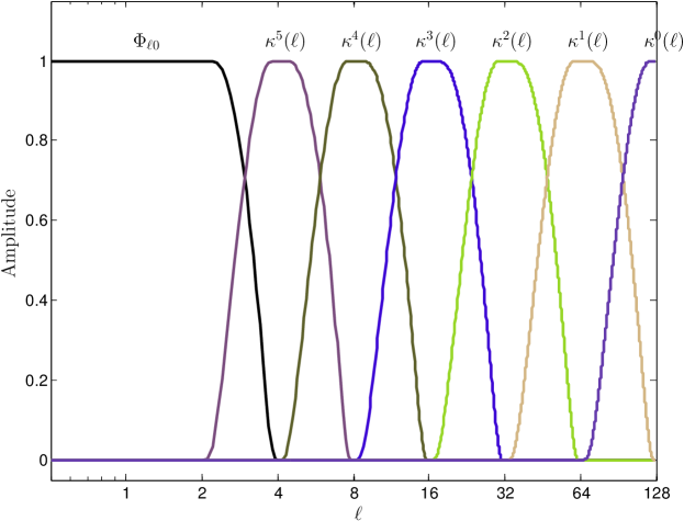
Figure 1: Scale-discretised wavelet tiling in harmonic space (${L}=128$, ${\lambda}=2$, ${N}=3$, $J=5$).

The maximum possible wavelet scale $J_{L}({\lambda})$ is given by the lowest integer $j$ for which the kernel peak occurs at or below $\ell=1$, i.e. by the lowest integer value such that ${\lambda}^{-J_{L}({\lambda})}{L}\leq 1$, yielding $J_{L}({\lambda})=\lceil\log_{\lambda}({L})\rceil$. All wavelets for $j>J_{L}({\lambda})$ would be identically null as their kernel would have compact support in $\ell\in(0,1)$. The maximum scale to be probed by the wavelets $J$ can be chosen within the range $0\leq J\leq J_{L}({\lambda})$. For $J=J_{L}({\lambda})$ the wavelets probe the entire frequency content of the signal of interest $f$ except its mean, encoded in ${f}_{{0}{0}}$ and incorporated in the scaling coefficients.

To represent the signal content not probed by the wavelets the scaling function $\Phi$ is required, as discussed previously. Recall that the scaling function $\Phi$ is chosen to be axisymmetric; hence, we define the harmonic coefficients of the scaling function by

$${\Phi}_{{\ell}{m}}\equiv\sqrt{\frac{2\ell+1}{4\pi}}\>\sqrt{k_{\lambda}({\lambda}^{J}{L}^{-1}\ell)}\>\delta_{{m}{0}}\>,$$ (18)

in order to ensure the scaling function probes the signal content not probed by the wavelets.

For the wavelets, scaling function and wavelet scale parameter ranges outlined above, the admissibility criterion Eq. (7) is satisfied. Although the precise construction of the directionality component has not yet been defined, provided it is normalised according to Eq. (13), admissibility holds.

3.2 Steerability

A function on the sphere is steerable if an azimuthal rotation of the function can be written as a linear combination of weighted basis functions. By imposing an azimuthal band-limit ${N}$ on the directionality component such that ${\zeta}_{{\ell}{m}}=0$, $\forall\ell,m$ with $|m|\geq{N}$, we recover wavelets that are steerable [81, 20]. Moreover, if $T\in\mathbb{N}$ of the harmonic coefficients ${\zeta}_{{\ell}{m}}$ are non-zero for a given $m$ for at least one $\ell$, then the number of basis functions $M\in\mathbb{N}$ required to steer the wavelet directionality component satisfies $M\geq T$ and the optimal number $M=T$ can be chosen. Furthermore, if $\zeta$ exhibits an azimuthal band-limit, then it can be steered using basis functions that are in fact rotations of itself:

$$\zeta_{\gamma}(\omega)=\sum_{g=0}^{M-1}z(\gamma-\gamma_{g})\>\zeta_{\gamma_{g}}(\omega)\>,$$ (19)

which extends to the wavelets $\Psi^{(j)}$ also, where $\zeta_{\gamma}\equiv\mathcal{R}_{(0,0,\gamma)}\zeta$ and $g\in\mathbb{N}$. The rotation angles $\gamma_{g}\in[0,2\pi)$ and interpolating function $z\in\mathrm{L}^{2}(\mathbb{R})$ are defined subsequently. Note that the interpolating function is independent of the directionality component $\zeta$ of the wavelet. Due to the linearity of the wavelet transform, the steerability property is transferred to the wavelet coefficients themselves, yielding

$$W^{\Psi^{(j)}}(\alpha,\beta,\gamma)=\sum_{g=0}^{M-1}z(\gamma-\gamma_{g})\>W^{\Psi^{(j)}}(\alpha,\beta,\gamma_{g})\>.$$ (20)

Before proving the steerability property of Eq. (19), we consider additional azimuthal symmetries that the directionality component, and thus wavelets, are designed to satisfy. For ${N}-1$ odd (even), the wavelets are constructed to exhibit odd (even) symmetry under a reflection of $\varphi$:

$$\zeta(\theta,-\varphi)=(-1)^{N-1}\>\zeta(\theta,\varphi)\>,$$ (21)

which for real functions on the sphere implies the harmonic coefficients ${\zeta}_{{\ell}{m}}$ are purely real for $N-1$ even and purely imaginary for $N-1$ odd. In addition, for ${N}-1$ odd (even), the wavelets are constructed to exhibit odd (even) symmetry under an azimuthal rotation by $\pi$:

$$\zeta(\theta,\varphi+\pi)=(-1)^{N-1}\>\zeta(\theta,\varphi)\>,$$ (22)

which implies the harmonic coefficients ${\zeta}_{{\ell}{m}}$ are zero for $m$ odd when ${N}-1$ is even and zero for $m$ even when ${N}-1$ is odd. This symmetry is exploited to optimise the number of basis functions required to steer the wavelet to $M=N$.

Returning to the steerability relation of Eq. (19), we prove this expression by proving the equivalent harmonic space representation:

$${(\zeta_{\gamma})}_{{\ell}{m}}=\sum_{m^{\prime}=-K}^{K}\sum_{n=-\ell}^{\ell}z_{m^{\prime}}\>{\rm exp}{({\rm i}m^{\prime}\gamma)}\>d_{mn}^{\ell}(0)\>{\zeta}_{{\ell}{n}}\sum_{g=0}^{M-1}{\rm exp}{(-i(m^{\prime}+n)\gamma_{g})}\>,$$ (23)

where $z_{m}$ are the Fourier coefficients of the interpolating function, $K\in\mathbb{N}$ is the (as yet unconstrained) band-limit of the interpolating function, and $d_{mn}^{\ell}$ are the Wigner $d$-functions (defined in A.1). Performing a rotation in harmonic space of the left-hand-side of Eq. (23), and noting the orthogonality of the final summation of Eq. (23) for the equiangular sampling $\gamma_{g}=g\pi/M$, with $m^{\prime},n<\lfloor M\rfloor$, and thus $K=\lfloor M\rfloor-1$, one finds that the steerability relation is satisfied provided $z_{m}=1/M=1/N$ over the domain where ${\zeta}_{{\ell}{m}}$ is non-zero and zero elsewhere, where we have exploited the symmetry relation of Eq. (22).

A steered wavelet for ${N}=3$ and its basis functions, given by rotated versions of the wavelet, are plotted in Fig. 2. The wavelet can be steered to any continuous orientation $\gamma$ by taking weighted sums of its three basis functions.

(a) $\gamma_{0}=0^{\circ}$

(b) $\gamma_{1}=60^{\circ}$

(c) $\gamma_{2}=120^{\circ}$

(d) Steered to $\gamma=30^{\circ}$

Figure 2: Demonstration of wavelet steerability property (${L}=256,\ {\lambda}=2,\ {N}=3,\ j=5$). The wavelet in panel (d) is steered by constructed from a weighted sum of the wavelets shown in panels (a)–(c) through Eq. (19).

3.3 Directional construction

(a) ${N}=1,\ j=6$

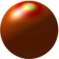
(b) ${N}=1,\ j=5$

(c) ${N}=1,\ j=4$

(d) ${N}=1,\ j=3$

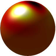
(e) ${N}=2,\ j=6$

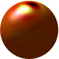
(f) ${N}=2,\ j=5$

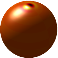
(g) ${N}=2,\ j=4$

(h) ${N}=2,\ j=3$

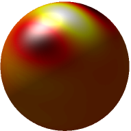
(i) ${N}=3,\ j=6$

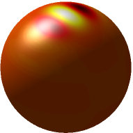
(j) ${N}=3,\ j=5$

(k) ${N}=3,\ j=4$

(l) ${N}=3,\ j=3$

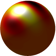
(m) ${N}=4,\ j=6$

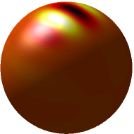
(n) ${N}=4,\ j=5$

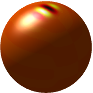
(o) ${N}=4,\ j=4$

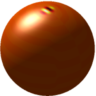
(p) ${N}=4,\ j=3$

Figure 3: Directional scale-discretised wavelets (${L}=256,\ {\lambda}=2,\ J=8$). Wavelet scale $j$ varies across columns, while azimuthal band-limit ${N}$ values across rows.

The directionality component is constructed to carefully control the directional localisation of the wavelet, while steerability is achieved by imposing an azimuthal band-limit ${N}$ (as described above). Directional localisation is controlled by imposing a specific form for the directional auto-correlation of the wavelet, where the directional auto-correlation is defined by

$$\Gamma^{{(j)}}(\Delta\gamma=\gamma^{\prime}-\gamma)\equiv\langle{\Psi^{(j)}_{\gamma}},\>{\Psi^{(j)}_{\gamma^{\prime}}}\rangle=\sum_{\ell=0}^{\infty}\>\bigl{|}\kappa^{(j)}(\ell)\bigr{|}^{2}\sum_{m=-\min(N-1,\ell)}^{\min(N-1,\ell)}\bigl{|}{\zeta}_{{\ell}{m}}\bigr{|}^{2}\>{\rm exp}{({\rm i}m\Delta\gamma)}\>,$$ (24)

where $\Psi^{(j)}_{\gamma}\equiv\mathcal{R}_{(0,0,\gamma)}\Psi^{(j)}$. The peakedness of the directional auto-correlation function can be considered as a measure of the directionality of the wavelet: the more peaked the directional auto-correlation, the more directional the wavelet [78, 81]. To control the directional localisation of the wavelet precisely, we seek a directional auto-correlation function of the form:

$$\Gamma^{{(j)}}(\Delta\gamma)=\sum_{\ell=0}^{\infty}\>\bigl{|}\kappa^{(j)}(\ell)\bigr{|}^{2}\>\cos^{p}(\Delta\gamma)\>.$$ (25)

The directionality component of the wavelet is then defined to satisfy

$$\cos^{p}(\Delta\gamma)=\sum_{m=-\min(N-1,\ell)}^{\min(N-1,\ell)}\>\bigl{|}{\zeta}_{{\ell}{m}}\bigr{|}^{2}\>{\rm exp}{({\rm i}m\Delta\gamma)}\>,$$ (26)

for $p\in\mathbb{N}$, where it is apparent that the modulus squared of the spherical harmonic coefficients of the directionality component identifies with the Fourier coefficients of $\cos^{p}(\Delta\gamma)$. By noting Euler’s formula and performing a binomial expansion, $\cos^{n}(\phi)$ can be written

$$\cos^{n}(\phi)=\frac{1}{2^{n}}\sum_{m=0}^{n}\>\biggl{(}{{n}\atop{m}}\biggr{)}\>{\rm exp}{\bigl{(}{\rm i}(n-2m)\phi\bigr{)}}\>,$$ (27)

for $\phi\in[0,2\pi)$, from which we recover the following Fourier series expansions for even and odd exponents, respectively:

$$\cos^{2n}(\phi)=\frac{1}{2^{2n}}\sum_{\begin{subarray}{c}m=-2n,\\ m\>\text{even}\end{subarray}}^{2n}\biggl{(}{{2n}\atop{n-m/2}}\biggr{)}\>{\rm exp}{({\rm i}m\phi)}$$ (28)

and

$$\cos^{2n+1}(\phi)=\frac{1}{2^{2n+1}}\sum_{\begin{subarray}{c}m=-(2n+1),\\ m\>\text{odd}\end{subarray}}^{2n+1}\biggl{(}{{2n+1}\atop{n-(m-1)/2}}\biggr{)}\>{\rm exp}{({\rm i}m\phi)}\>.$$ (29)

Associating the Fourier coefficients of cosine raised to a power with the harmonic coefficients of the directionality component of the wavelet, the following coherent expression is recovered for both even and odd exponents:

$${\zeta}_{{\ell}{m}}=\eta\>\upsilon\>\sqrt{\frac{1}{2^{p}}\biggl{(}{{p}\atop{(p-m)/2}}\biggr{)}}\>,$$ (30)

where

$$\eta=\begin{cases}1,&\text{if ${N}-1$ even}\\ {\rm i},&\text{if ${N}-1$ odd}\end{cases}\>,$$ (31)

$$\upsilon=[1-(-1)^{{N}+m}]/2=\begin{cases}0,&\text{if ${N}+m$ even}\\ 1,&\text{if ${N}+m$ odd}\end{cases}$$ (32)

and

$$p=\min\{{N}-1,\ell-[1+(-1)^{{N}+\ell}]/2\}=\begin{cases}\min({N}-1,\ell-1),&\text{if ${N}+\ell$ even}\\ \min({N}-1,\ell),&\text{if ${N}+\ell$ odd}\end{cases}\>.$$ (33)

The factors $\eta$ and $\upsilon$ are introduced to ensure the symmetries given by Eq. (21) and Eq. (22), respectively, are satisfied. The exponent $p$ is defined to achieve the greatest directionality supported by the azimuthal band-limit available at a given $\ell$. For wavelets with support within $\ell\geq{N}$, i.e. $j\leq J_{N}=\lfloor\log_{\lambda}({L}/{N})-1\rfloor$, (which is usually the case since ${N}$ is typically chosen to be relatively small and the scaling function is used to represent the approximation-information of the signal), the parameter $p$ is given by ${N}-1$ and becomes independent of $\ell$. Note that the directional component normalisation of Eq. (13) is satisfied since $\sum_{k}\bigl{(}{{n}\atop{k}}\bigr{)}=2^{n}$. Example wavelets are plotted in Fig. 3, while directional auto-correlation functions are plotted in Fig. 4.

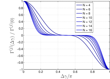
(a) Odd $N-1$

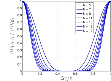
(b) Even $N-1$

Figure 4: Directional auto-correlation for even and odd ${N}-1$. As ${N}$ increases the directional auto-correlation function becomes more peaked and the associated wavelet more directional.

4 Localisation properties

We show in this section that directional scale-discretised wavelets $\Psi^{(j)}$ are characterised by an excellent localisation property in the spatial domain. More precisely, for any $\xi\in\mathbb{R}^{+}_{\ast}$, there exists strictly positive $C_{\xi,{N}}\in\mathbb{R}^{+}_{\ast}$, such that the local concentration of a directional wavelet centred on the North pole reads:

$$\bigl{|}\Psi^{(j)}(\theta,\varphi)\bigr{|}\leq\frac{\bigl{(}L\lambda^{-j}\bigr{)}^{2+{N}}C_{\xi,{N}}}{\bigl{(}1+L\lambda^{-j}\theta\bigr{)}^{\xi}}\>.$$ (34)

For the sake of simplicity, we present here the outline of the proof of this property; all the mathematical technicalities are extensively described in A.

Firstly, observe the following decomposition of directional scale-discretised wavelets in terms of spherical harmonics:

$$\Psi^{(j)}(\omega)=\sum_{\ell=0}^{\infty}\sum_{m=-\ell}^{\ell}\kappa^{(j)}(\ell)\>\zeta_{\ell m}\>\sqrt{\frac{2\ell+1}{8\pi^{2}}}\>Y_{\ell m}({\omega})\>.$$ (35)

For our purposes, we recall a general result in mathematical analysis, namely Theorem 2.2 of [25], which states that the spatial concentration properties of such wavelet constructions are conserved under the action of $C^{\infty}$-differential operators, up to a polynomial term depending on the degree of the operator. A full statement of the theorem can be found in A.2. In order to apply this result, we rewrite directional wavelets in terms of some proper differential operator.

Let us start by assuming, for the sake of simplicity, that $\zeta_{\ell m}$ does not depend on the multipole $\ell$ but just on the azimuthal angle. For wavelet scales $j\leq J_{N}=\lfloor\log_{\lambda}({L}/{N})-1\rfloor$ such that the harmonic support of the wavelet lies within $\ell\geq N$ (the standard setting), this assumption is satisfied directly (as discussed in Section 3.3). For $\ell<N$, straightforward calculations lead to:

$$\zeta_{\ell m}\leq\left(\frac{\ell}{\sqrt{2}}\right)^{-\frac{1}{4}}\leq 1,\text{ for }\ell>1\>.$$ (36)

Consequently, from now on we will write $\zeta_{m}\equiv\zeta_{\ell m}$.

Let us define the following $C^{\infty}$-differential operator on $\theta$ of order $m$ on the sphere:

$$\mathcal{T}_{m}\equiv(\sin\theta)^{m}\frac{\partial^{m}}{\partial(\cos\theta)^{m}}=\sum_{k=0}^{m}a_{k}\sin^{k}\theta\frac{\partial^{k}}{\partial\theta^{k}}\>.$$ (37)

Following Eq. (81) in A.1, we can rewrite the wavelet as

$$\Psi^{(j)}(\theta,\varphi)=\sum_{m=-{N}}^{{N}}\zeta_{m}\>{\rm exp}{({\rm i}m\varphi)}\left(-1\right)^{m}\sum_{\ell=(L\lambda^{-(1+j)}\vee m)}^{L\lambda^{1-j}}\kappa^{(j)}(\ell)\>\frac{2\ell+1}{2^{5/2}\pi^{3/2}}\sqrt{\frac{(\ell-m)!}{(\ell+m)!}}\>\mathcal{T}_{m}P_{\ell}(\cos\theta)\>,$$ (38)

where $P_{\ell}(\cdot)$ are the Legendre polynomials (defined in A.1) and we have adopted the shorthand notation $a\vee b=\max(a,b)$. Straightforward manipulations lead to the following bound, for any $\varphi$:

$$\bigl{|}\Psi^{(j)}(\theta,\varphi)\bigr{|}\leq(2{N}+1)\max_{m=-{N},...,{N}}\>\bigl{|}\zeta_{m}\bigr{|}\>\bigl{|}Q_{m}^{(j)}(\cos\theta)\bigr{|}\>,$$ (39)

where

$$Q_{m}^{(j)}(\cos\theta)\equiv\sum_{\ell=(L\lambda^{-(1+j)}\vee m)}^{L\lambda^{1-j}}\kappa^{(j)}(\ell)\>\frac{2\ell+1}{2^{7/2}\pi^{5/2}}\>\ell^{-m}\>\mathcal{T}_{m}P_{\ell}(\cos\theta)\>.$$ (40)

We have employed the bound of Eq. (110) above, which is derived in A.3.

For the sake of simplicity, let $\varepsilon_{j}=\lambda^{j}L^{-1}$ and define the function $b_{m,\varepsilon_{j}}$ mapping $\mathbb{R}$ to $\mathbb{R^{+}}$ as

$$b_{m,\varepsilon_{j}}(x)\equiv\kappa^{(j)}(x)\>x^{-m},\text{ for }x>0\>.$$ (41)

As in [55], we extend this function to the negative axis simply by taking $b_{m,\varepsilon_{j}}(-|x|)=b_{m,\varepsilon_{j}}(|x|)$. Furthermore, because the function $\kappa^{(j)}$ assumes the value $0$ in the interval $(-{\lambda}^{-(1+j)}{L},{\lambda}^{-(1+j)}{L})$, it also holds that $b_{m,\varepsilon_{j}}(x)=0$ for $x\in(-{\lambda}^{-(1+j)}{L},0)\cup(0,{\lambda}^{-(1+j)}{L})$. Moreover, we extend for continuity $b_{m,\varepsilon_{j}}(0)=0$.

We then obtain:

$$Q_{m}^{(j)}(\cos\theta)=\frac{1}{\left(2\pi\right)^{5/2}}\mathcal{T}_{m}U^{\left(j\right)}_{m}(\cos\theta)\>,$$ (42)

where

$$U^{\left(j\right)}_{m}(\cos\theta)\equiv\sum_{\ell=(L\lambda^{-(1+j)}\vee m)}^{L\lambda^{1-j}}b_{m,\varepsilon_{j}}(\ell)\Bigl{(}\ell+\frac{1}{2}\Bigr{)}P_{\ell}(\cos\theta)\>.$$ (43)

As proved in A.4, for any $\xi\in\mathbb{R}^{+}_{\ast}$, there exists $C_{\xi}\in\mathbb{R}^{+}_{\ast}$ such that $U^{\left(j\right)}_{m}(\cos\theta)$ is bounded above:

$$\bigl{|}U^{\left(j\right)}_{m}(\cos\theta)\bigr{|}\leq\frac{C_{\xi}/\varepsilon_{j}^{2}}{\Bigl{(}1+\bigl{|}\frac{\theta}{\varepsilon_{j}}\bigr{|}\Bigr{)}^{\xi}}\>.$$ (44)

According to Eq. (108) of A.2 it follows that

$$\bigl{|}Q^{(j)}_{m}(\cos\theta)\bigr{|}\leq\frac{(L\lambda^{-j})^{2+m}C_{\xi}}{\bigl{(}1+L\lambda^{-j}\theta\bigr{)}^{\xi}}\>,$$ (45)

and, therefore, we obtain

$$\bigl{|}\Psi^{(j)}(\theta,\varphi)\bigr{|} \leq(2{N}+1)\max_{m=-{N},...,{N}}\>\bigl{|}\zeta_{m}\bigr{|}\>\frac{(L\lambda^{-j})^{2+{N}}C_{\xi}}{\bigl{(}1+L\lambda^{-j}\theta\bigr{)}^{\xi}}$$ (46)

$$\leq\frac{(L\lambda^{-j})^{2+{N}}C_{\xi,{N}}}{\bigl{(}1+L\lambda^{-j}\theta\bigr{)}^{\xi}}\>,$$ (47)

as claimed.

If we consider spin scale-discretised wavelets [46], denoted by ${}_{s}\Psi^{(j)}(\omega)$, $\omega\in{\mathbb{S}^{2}}$, the following decomposition in terms of spin spherical harmonics ${{}_{s}Y_{\ell m}({\omega})}$ holds:

$${}_{s}\Psi^{(j)}(\omega)=\sum_{\ell=0}^{\infty}\sum_{m=-\ell}^{\ell}\kappa^{(j)}(\ell)\>\zeta_{\ell m}\>\sqrt{\frac{2\ell+1}{8\pi^{2}}}\>{{}_{s}Y_{\ell m}({\omega})}\>.$$ (48)

Details and properties concerning spin spherical harmonics are extensively discussed in the A.1. Considering $s>0$, and using Eq. (97), we obtain

$${}_{s}\Psi^{(j)}(\omega)=\sum_{\ell=0}^{\infty}\sum_{m=-\ell}^{\ell}\kappa^{(j)}(\ell)\>\zeta_{\ell m}\>\sqrt{\frac{2\ell+1}{8\pi^{2}}}\ \biggl{[}\frac{(\ell-s)!}{(\ell+s)!}\biggr{]}^{1/2}\eth^{s}Y_{\ell m}({\omega})\>\>.$$ (49)

Observe that $\bigl{[}{(\ell-s)!}/{(\ell+s)!}\bigr{]}^{1/2}$ is bounded by $\ell^{-s}$, as given by Eq. (110) and shown in A.3. Noting Eq. (79), Eq. (80) and Eq. (81), straightforward calculations, entirely analogous to the scalar case and therefore omitted for the sake of brevity, lead to the following inequality:

$$\bigl{|}{}_{s}\Psi^{(j)}(\theta,\varphi)\bigr{|}\leq(2{N}+1)\max_{m=-{N},...,{N}}\>\bigl{|}\zeta_{m}\bigr{|}\>\bigl{|}{}_{s}Q_{m}^{(j)}(\cos\theta)\bigr{|}\>,$$ (50)

where

$${}_{s}Q_{m}^{(j)}(\cos\theta)\equiv\sum_{\ell=(L\lambda^{-(1+j)}\vee m)}^{L\lambda^{1-j}}\kappa^{(j)}(\ell)\>\frac{2\ell+1}{2^{7/2}\pi^{5/2}}\>\ell^{-(m+s)}\>\eth^{s}\mathcal{T}_{m}P_{\ell}(\cos\theta)\>.$$ (51)

Similar manipulations of ${}_{s}Q_{m}^{(j)}(\cos\theta)$ to those presented above (see again A.2), lead to the following result. For any $\xi\in\mathbb{R}^{+}_{\ast}$, there exists a strictly positive $C_{\xi,{N},s}\in\mathbb{R}^{+}_{\ast}$ such that

$$\bigl{|}{}_{s}\Psi^{(j)}(\theta,\varphi)\bigr{|} \leq\frac{(L\lambda^{-j})^{2+{N}+s}C_{\xi,{N},s}}{\bigl{(}1+L\lambda^{-j}\theta\bigr{)}^{\xi}}\>.$$ (52)

5 Stochastic properties

We study in this section the stochastic properties of zero-mean homogeneous and isotropic Gaussian random fields on the sphere $f$ when decomposed by directional scale-discretised wavelets. The stochastic field $f$ is characterised by its power spectrum $C_{\ell}$, with

$$\mathbb{E}({f}_{{\ell}{m}}{f}_{{\ell^{\prime}}{m^{\prime}}}^{\ast})=C_{\ell}\>\delta_{{\ell}{\ell^{\prime}}}\delta_{{m}{m^{\prime}}}$$ (53)

and

$$\mathbb{E}({f}_{{\ell}{m}})=0\>.$$ (54)

Specifically, we study the correlation of directional scale-discretised wavelet coefficients given by

$$\Xi^{(jj^{\prime})}(\mathbf{\rho}_{1},\mathbf{\rho}_{2})\equiv\frac{\mathbb{E}\Bigl{[}W^{\Psi^{(j)}}(\mathbf{\rho}_{1})\>W^{\Psi^{(j^{\prime})}}{}^{\ast}(\mathbf{\rho}_{2})\Bigr{]}}{\sqrt{\mathbb{E}\biggl{[}\Bigl{|}W^{\Psi^{(j)}}(\mathbf{\rho}_{1})\Bigr{|}^{2}\biggr{]}}\sqrt{\mathbb{E}\biggl{[}\Bigl{|}W^{\Psi^{(j^{\prime})}}(\mathbf{\rho}_{2})\Bigr{|}^{2}\biggr{]}}}\>.$$ (55)

For notational convenience, we also introduce the covariance

$$\xi^{(jj^{\prime})}(\mathbf{\rho}_{1},\mathbf{\rho}_{2})\equiv\mathbb{E}\Bigl{[}W^{\Psi^{(j)}}(\mathbf{\rho}_{1})\>W^{\Psi^{(j^{\prime})}}{}^{\ast}(\mathbf{\rho}_{2})\Bigr{]}\>,$$ (56)

such that

$$\Xi^{(jj^{\prime})}(\mathbf{\rho}_{1},\mathbf{\rho}_{2})=\frac{\xi^{(jj^{\prime})}(\mathbf{\rho}_{1},\mathbf{\rho}_{2})}{\sqrt{\xi^{(jj)}(\mathbf{\rho}_{1},\mathbf{\rho}_{1})\>\xi^{(j^{\prime}j^{\prime})}(\mathbf{\rho}_{2},\mathbf{\rho}_{2})}}\>.$$ (57)

Recall the harmonic representation of the scale-discretised wavelet transform of Eq. (9). Noting this expansion, the wavelet covariance may be written

$$\xi^{(jj^{\prime})}(\mathbf{\rho}_{1},\mathbf{\rho}_{2}) =\sum_{\ell=0}^{\infty}\sum_{n=-\ell}^{\ell}\sum_{n^{\prime}=-\ell}^{\ell}C_{\ell}\>{\Psi}_{{\ell}{n}}^{(j)\ast}\>{\Psi}_{{\ell}{n^{\prime}}}^{(j^{\prime})}\sum_{m=-\ell}^{\ell}D_{mn}^{\ell\ast}(\mathbf{\rho}_{1})\>D_{mn^{\prime}}^{\ell}(\mathbf{\rho}_{2})$$ (58)

$$=\sum_{\ell=0}^{\infty}\sum_{n=-\ell}^{\ell}\sum_{n^{\prime}=-\ell}^{\ell}C_{\ell}\>{\Psi}_{{\ell}{n}}^{(j)\ast}\>{\Psi}_{{\ell}{n^{\prime}}}^{(j^{\prime})}\>D_{nn^{\prime}}^{\ell}(\mathbf{\rho})\>,$$ (59)

where the second line follows from Eq. (91) and $\mathbf{R}_{\mathbf{\rho}}=\mathbf{R}_{\mathbf{\rho}_{1}}^{-1}\mathbf{R}_{\mathbf{\rho}_{2}}$ (see A.1 for further details). For the case where $\mathbf{\rho}_{1}=\mathbf{\rho}_{2}$ and $j^{\prime}=j$, the covariance reduces to

$$\xi^{(jj)}(\mathbf{\rho},\mathbf{\rho})=\sum_{\ell=0}^{\infty}\sum_{n=-\ell}^{\ell}C_{\ell}\>\bigl{|}{\Psi}_{{\ell}{n}}^{(j)}\bigr{|}^{2}\>,$$ (60)

by Eq. (93) of A.1 (as also shown in [49]).

Expressing the wavelet by its kernel and directionality component, the wavelet covariance reads:

$$\xi^{(jj^{\prime})}(\mathbf{\rho}_{1},\mathbf{\rho}_{2})=\sum_{\ell=0}^{\infty}\sum_{n=-\ell}^{\ell}\sum_{n^{\prime}=-\ell}^{\ell}C_{\ell}\>\frac{2\ell+1}{8\pi^{2}}\>\kappa^{(j)}(\ell)\>\kappa^{(j^{\prime})}(\ell)\>{\zeta}_{{\ell}{n}}\>{\zeta}_{{\ell}{n^{\prime}}}\>D_{nn^{\prime}}^{\ell}(\mathbf{\rho})$$ (61)

Furthermore, using Eq. (81), we obtain

$$\xi^{(jj^{\prime})}(\mathbf{\rho}_{1},\mathbf{\rho}_{2})=\xi_{(+)}^{(jj^{\prime})}(\mathbf{\rho}_{1},\mathbf{\rho}_{2})+\xi_{(-)}^{(jj^{\prime})}(\mathbf{\rho}_{1},\mathbf{\rho}_{2}),$$ (62)

where

$$\xi_{(+)}^{(jj^{\prime})}(\mathbf{\rho}_{1},\mathbf{\rho}_{2})= \sum_{\ell=0}^{\infty}\sum_{n=-\ell}^{\ell}\sum_{n^{\prime}=0}^{\ell}C_{\ell}\>\frac{2\ell+1}{2^{7/2}\pi^{5/2}}\kappa^{(j)}(\ell)\kappa^{(j^{\prime})}(\ell){\zeta}_{{\ell}{n}}{\zeta}_{{\ell}{n^{\prime}}}$$

$$\times(-1)^{n}\sqrt{\frac{(\ell-n^{\prime})!(\ell-n)!}{(\ell+n^{\prime})!(\ell+n^{\prime})!}}\>{\rm exp}{\bigl{(}{\rm i}(-n\alpha+n^{\prime}\gamma)\bigr{)}}\>\bar{\eth}^{n^{\prime}}\>\mathcal{T}_{n}\>P_{{\ell}}({\cos\beta})$$ (63)

and

$$\xi_{(-)}^{(jj^{\prime})}(\mathbf{\rho}_{1},\mathbf{\rho}_{2})= \sum_{\ell=0}^{\infty}\sum_{n=-\ell}^{\ell}\sum_{n^{\prime}=-\ell}^{-1}C_{\ell}\>\frac{2\ell+1}{2^{7/2}\pi^{5/2}}\kappa^{(j)}(\ell)\kappa^{(j^{\prime})}(\ell){\zeta}_{{\ell}{n}}{\zeta}_{{\ell}{n^{\prime}}}$$

$$\times\sqrt{\frac{(\ell-|n^{\prime}|)!(\ell-n)!}{(\ell+|n^{\prime}|)!(\ell+n^{\prime})!}}\>{\rm exp}{\bigl{(}{\rm i}(-n\alpha+n^{\prime}\gamma)\bigr{)}}\>\bar{\eth}^{|n^{\prime}|}\>\mathcal{T}_{n}\>P_{{\ell}}({\cos\beta}),$$ (64)

where in Eq. (63) we applied Eq. (100), while in Eq. (64) we applied Eq. (101). In both those formulas and henceforth, $\beta$ is the Euler angle associated to the resultant rotation $\mathbf{\rho}=(\alpha,\beta,\gamma)$, as stated above. These expression show that, up to a complex exponential factor, both $\xi_{(+)}^{(jj^{\prime})}(\mathbf{\rho}_{1},\mathbf{\rho}_{2})$ and $\xi_{(-)}^{(jj^{\prime})}(\mathbf{\rho}_{1},\mathbf{\rho}_{2})$ depend on the absolute value of $n^{\prime}$.

Following, for instance, [6], we introduce some mild regularity conditions on $C_{\ell}$ (see also [35]). Assume there exists $R\in\mathbb{N}$, $\alpha\in\mathbb{R}$, $\alpha\geq 2$ and a sequence of functions $\bigl{\{}g^{(\lambda)}_{j}(\cdot)\bigr{\}}$ such that we can rewrite

$$C_{\ell}=\ell^{-\alpha}g_{j}^{(\lambda)}(\lambda^{j}L^{-1}\ell)>0\>,$$ (65)

for $\ell\in\bigl{[}\lfloor{\lambda}^{-(1+j)}{L}\rfloor,\lceil{\lambda}^{1-j}{L}\rceil\bigr{]}$ and for $j\in\mathbb{N}$, $0<g_{j}^{(\lambda)}<\infty$, while for $r=1,\ldots,R$, there exists $c_{r}\in\mathbb{R}^{+}$ such that

$$\sup_{j\in\mathbb{N}}\>\sup_{u\in[L\lambda^{-1},L\lambda]}\>\Bigl{|}\frac{d^{r}}{du^{r}}g_{j}^{(\lambda)}(u)\Bigr{|}\leq c_{r}\>.$$ (66)

These conditions guarantee the boundedness and smoothness of $C_{\ell}$ and are useful in the context of practical applications. For instance, these conditions encompass standard cosmological models describing the CMB, where the CMB is modelled as a realisation of a Gaussian random field on the sphere and where $C_{\ell}$ can be modelled approximately by inverse polynomials (cf. [16]). Note also that, as stated in [6], the sequence $\bigl{\{}g^{(\lambda)}_{j}(\cdot)\bigr{\}}$ belongs to the Sobolev space $W^{R,\infty}$. Because it follows immediately that there should exist $g_{1},g_{2},\alpha\in\mathbb{R^{+}}$, $\alpha\geq 2$, such that $g_{1}\ell^{-\alpha}\leq C_{\ell}\leq g_{1}\ell^{-\alpha}$, for the sake of the simplicity and without losing any generality, we assume henceforth $C_{\ell}=g_{1}\ell^{-\alpha}$ (see, again, [6]).

Consider now the variance: in order to compute its lower bound, observe that, for $\ell$ sufficiently large, the following integral approximation holds

$$\sum_{\ell=0}^{\infty}(\lambda^{j}L^{-1}\ell)^{-\alpha}\>(\lambda^{j}L^{-1})^{2}\left(2\ell+1\right)\>\bigl{(}\kappa^{(j)}(\ell)\bigr{)}^{2}\> =\sum_{\ell=\lfloor{\lambda}^{-(1+j)}{L}\rfloor}^{\lceil{\lambda}^{1-j}{L}\rceil}\>(\lambda^{j}L^{-1}\ell)^{-\alpha}\>(\lambda^{j}L^{-1})^{2}\left(2\ell+1\right)\>\bigl{(}\kappa_{\lambda}(\lambda^{j}L^{-1}\ell)\bigr{)}^{2}\>$$

$$\simeq 2\int_{\lambda^{-1}}^{\lambda}x^{1-\alpha}\>\bigl{(}\kappa_{\lambda}(x)\bigr{)}^{2}\mathrm{\,d}x\>,$$ (67)

where $0<C_{1}\leq 2\int_{\lambda^{-1}}^{\lambda}x^{1-\alpha}\>\bigl{(}\kappa_{\lambda}(x)\bigr{)}^{2}\mathrm{\,d}x\leq C_{2}<\infty$, and $C_{1},C_{2}\in\mathbb{R^{+}}$ (cf. Lemma 3 in [6]). Recalling $\sum_{n=-\ell}^{\ell}\bigl{|}\zeta_{n}\bigr{|}^{2}=1$, straightforward manipulations lead us to the following inequality:

$$\xi^{(jj)}(\mathbf{\rho},\mathbf{\rho})=\sum_{\ell=0}^{\infty}C_{\ell}\>\frac{2\ell+1}{8\pi^{2}}\>\bigl{(}\kappa^{(j)}(\ell)\bigr{)}^{2}\geq C_{1}(L\lambda^{-j})^{(2-\alpha)}.$$ (68)

As far as the correlation $\xi^{(jj^{\prime})}(\mathbf{\rho}_{1},\mathbf{\rho}_{2})$ is concerned, observe that $\kappa^{(j)}(\ell)\kappa^{(j^{\prime})}(\ell)=0$ if $|j-j^{\prime}|>1$, so that $\xi^{(jj^{\prime})}(\mathbf{\rho}_{1},\mathbf{\rho}_{2})$ is different from $0$ only if $j^{\prime}=j$ or if $j^{\prime}=j\pm 1$.

Let us consider $j=j^{\prime}$ and define a sequence of functions $\phi_{\lambda,1}^{(j)}$ given by $\phi_{\lambda,1}^{(j)}(u)=\bigl{(}\kappa^{(j)}(u)\bigr{)}^{2}g_{j}^{(\lambda)}(u)u^{-\alpha-n-n^{\prime}}$. Assuming again that ${\zeta}_{{\ell}{n}}=\zeta_{n}$, we have

$$\xi_{(+)}^{(jj)}(\mathbf{\rho}_{1},\mathbf{\rho}_{2})\leq\sum_{n}\sum_{n^{\prime}}\zeta_{n}\zeta_{n^{\prime}}\sum_{l}\frac{2\ell+1}{2^{7/2}\pi^{5/2}}\>\phi_{\lambda,1}^{(j)}(\ell)\>\bar{\eth}^{n^{\prime}}\mathcal{T}_{n}P_{{\ell}}({\cos\beta})\>.$$ (69)

A similar result is attained as far as $\xi_{(-)}^{(jj)}(\mathbf{\rho}_{1},\mathbf{\rho}_{2})$ is concerned. Recalling that both $n$ and $n^{\prime}$ are bounded by ${N}$, we apply again the same techniques used to achieve localisation in Section 4, where $\phi_{\lambda,1}^{(j)}(\ell)$ plays the same role as $b_{m,\epsilon_{j}}\left(\ell\right)$ in Eq. (42), here omitted for the sake of brevity. These considerations lead to the following result. For any $\xi^{\prime}\in\mathbb{R}^{+}$, $\xi^{\prime}\geq 2(1+{N})$, there exists $C_{\xi^{\prime},M}$ such that

$$\xi^{(jj)}(\mathbf{\rho}_{1},\mathbf{\rho}_{2})\leq\frac{(L\lambda^{-j})^{2(1+{N})-\alpha}C_{\xi^{\prime},{N}}}{\bigl{(}1+L\lambda^{-j}\beta\bigr{)}^{\xi^{\prime}}}\>.$$ (70)

Combining Eq. (75) and Eq. (70), we attain the following bound. For any $\xi^{\prime\prime}\in\mathbb{R}^{+}$, $\xi^{\prime\prime}\geq 2{N}$, there exists $C_{\xi^{\prime\prime},M}$ such that

$$\Xi^{(jj)}(\mathbf{\rho}_{1},\mathbf{\rho}_{2})\leq\frac{(L\lambda^{-j})^{2{N}}C_{\xi^{\prime\prime},{N}}}{\bigl{(}1+L\lambda^{-j}\beta\bigr{)}^{\xi^{\prime\prime}}}\>.$$ (71)

Likewise, let us suppose $j^{\prime}=j-1$, remarking that the case $j^{\prime}=j+1$ is entirely analogous. Let us define a sequence of functions $\phi_{\lambda,2}^{(j)}$ given by $\phi_{\lambda,1}^{(j)}(u)=\kappa^{(j)}(u)\kappa^{(j-1)}(u)g_{j}^{(\lambda)}(u)u^{-\alpha-n-n^{\prime}}$. Again recalling that ${\zeta}_{{\ell}{n}}=\zeta_{n}$, we have

$$\xi_{(+)}^{(j,j-1)}(\mathbf{\rho}_{1},\mathbf{\rho}_{2})\leq\sum_{n}\sum_{n^{\prime}}\zeta_{n}\zeta_{n^{\prime}}\sum_{l}\frac{2\ell+1}{8\pi^{2}}\>\phi_{\lambda,2}^{(j)}(\ell)\>\bar{\eth}^{n^{\prime}}\mathcal{T}_{n}P_{{\ell}}({\cos\beta}).$$ (72)

Straightforward calculations, similar to the case $j=j^{\prime}$, provide an identical bound for $\Xi^{(j,j^{\prime})}(\mathbf{\rho}_{1},\mathbf{\rho}_{2})$ .

Therefore, for the sake of the clarity, we state directly the final result: for any $j,j^{\prime}\in\mathbb{N}$ such that $\left|j-j^{\prime}\right|<2$ and for any $\xi_{0}\in\mathbb{R}^{+}$, $\xi_{0}\geq 2{N}$, there exists $C_{\xi_{0},M}$ such that

$$\Xi^{(jj^{\prime})}(\mathbf{\rho}_{1},\mathbf{\rho}_{2})\leq\frac{(L\lambda^{-j})^{2{N}}C_{\xi_{0},{N}}}{\bigl{(}1+L\lambda^{-j}\beta\bigr{)}^{\xi_{0}}}\>.$$ (73)

As far as spin scale-discretised wavelets are concerned [46], consider an isotropic spin $s$ random field ${}_{s}f\in{\mathbb{S}^{2}}$ and its corresponding spherical harmonic coefficients ${}_{s}f_{\ell m}=\langle f_{s},{}_{s}Y_{\ell m}\rangle$. As proved in Theorem 7.2 of [23], it holds that $\mathbb{E}({}_{s}f_{\ell m}{}_{s}f_{\ell^{\prime}m^{\prime}}^{*})=C_{\ell}\delta_{{\ell}{\ell^{\prime}}}\delta_{{m}{m^{\prime}}}$, where $C_{\ell}$ is the spin power spectrum, which is invariant with respect to the choice of the system of coordinates over ${\mathbb{S}^{2}}$ (see also [24]). Therefore, the upper bound established for the correlation between spin directional scale-discretised wavelet coefficients is entirely analogous to the one developed for the scalar case. Indeed, the spin wavelet correlation becomes

$${}_{s}\xi^{(jj^{\prime})}(\mathbf{\rho}_{1},\mathbf{\rho}_{2}) =\sum_{\ell=0}^{\infty}\sum_{n=-\ell}^{\ell}\sum_{n^{\prime}=-\ell}^{\ell}C_{\ell}\>{}_{s}{\Psi}_{{\ell}{n}}^{(j)\ast}\>{}_{s}{\Psi}_{{\ell}{n^{\prime}}}^{(j^{\prime})}\>D_{nn^{\prime}}^{\ell}(\mathbf{\rho})\>,$$ (74)

and the wavelet variance is bounded as

$${}_{s}\xi^{(jj)}(\mathbf{\rho},\mathbf{\rho})=\sum_{\ell=0}^{\infty}C_{\ell}\>\frac{2\ell+1}{8\pi^{2}}\>\bigl{(}\kappa^{(j)}(\ell)\bigr{)}^{2}\geq C_{1}(L\lambda^{-j})^{(2-\alpha)},$$ (75)

because $\sum_{m=-\ell}^{\ell}{}_{s}Y_{\ell m}\left(\omega\right){}_{s}Y_{\ell m}^{*}\left(\omega\right)=\frac{2\ell+1}{4\pi}$, for any $\omega\in{\mathbb{S}^{2}}$. Straightforward calculations lead to the following result. For any $j,j^{\prime}\in\mathbb{N}$ such that $\left|j-j^{\prime}\right|<2$ and for any $\xi_{0}^{\prime}\in\mathbb{R}^{+}$, $\xi_{0}^{\prime}\geq 2{N}$, there exists $C_{\xi_{0}^{\prime},M}$ such that

$${}_{s}\Xi^{(jj^{\prime})}(\mathbf{\rho}_{1},\mathbf{\rho}_{2})\leq\frac{(L\lambda^{-j})^{2{N}}C_{\xi_{0}^{\prime},{N}}}{\bigl{(}1+L\lambda^{-j}\beta\bigr{)}^{\xi_{0}^{\prime}}}\>.$$ (76)

6 Numerical experiments

We perform numerical experiments to study the localisation and correlation properties of directional scale-discretised wavelet coefficients of simulations of homogenous and isotropic Gaussian random fields on the sphere. Specifically, we simulate realisations of the the CMB, which, in the standard Lambda Cold Dark Matter ($\Lambda$CDM) cosmological model, is assumed to be a realisation of a Gaussian random field on the sphere. We assume a power spectrum $C_{\ell}$ specified by the $\Lambda$CDM cosmological model that best fits observations of the CMB made by NASA’s Wilkinson Microwave Anisotropy Probe (WMAP) [28] (combined with other cosmological data: we adopt the full 9-year WMAP$+$BAO$+$H0 best-fit 6 parameter $\lambda$CDM model). Our Milky Way galaxy obscures our view of the CMB, hence real observations are made over incomplete sky coverage. We study statistical properties of wavelet coefficients in the presence of incomplete coverage on the sphere, adopting the WMAP KQ75 mask [8] (see Fig. 5). To compute directional scale-discretised wavelet transforms on the sphere we use the s2let code [33, 46], which in turn relies on the so3 [38] and ssht [51] codes, all of which are open-source and publicly available.

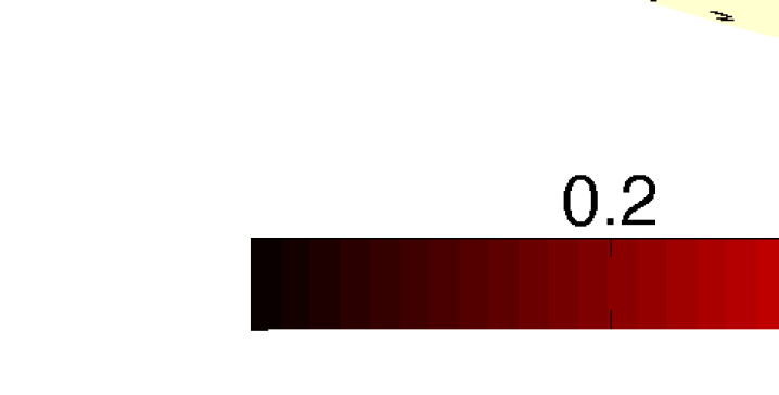
Figure 5: Binary (WMAP9 KQ75) mask plotted using the Mollweide projection showing regions of the sky where the CMB is accurately observable (ones of mask) and unobservable (zeros of mask).

6.1 Localisation

(a) $\gamma=0^{\circ}$

(b) $\gamma=60^{\circ}$

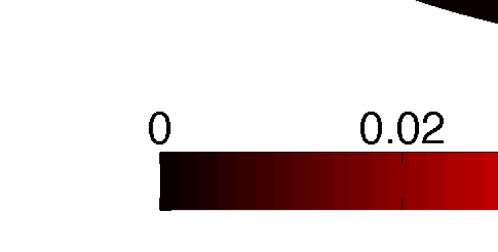
(c) $\gamma=120^{\circ}$

Figure 6: Localisation statistic $\Delta^{{(j)}}(\mathbf{\rho})$, plotted using a Mollweide projection for each orientation $\gamma$, computed from Monte Carlo simulations (${L}=128,\ {\lambda}=2,\ {N}=3,\ j=2$).

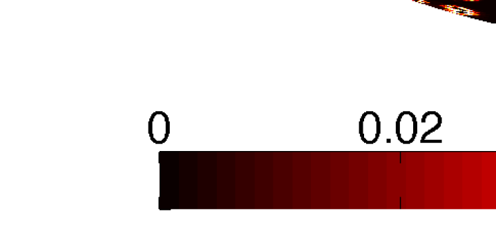
(a) $\gamma=0^{\circ}$

(b) $\gamma=60^{\circ}$

(c) $\gamma=120^{\circ}$

Figure 7: Localisation statistic $\Delta^{{(j)}}(\mathbf{\rho})$, plotted using a Mollweide projection for each orientation $\gamma$, computed from Monte Carlo simulations (${L}=256,\ {\lambda}=2,\ {N}=3,\ j=2$).

To study localisation properties in the context of incomplete coverage we compute the following localisation statistic:

$$\Delta^{(j)}(\mathbf{\rho})=\frac{\mathbb{E}\biggl{[}\Bigl{|}\widehat{W}^{\Psi^{(j)}}(\mathbf{\rho})-W^{\Psi^{(j)}}(\mathbf{\rho})\Bigr{|}^{2}\biggr{]}}{\mathbb{E}\biggl{[}\Bigl{|}W^{\Psi^{(j)}}(\mathbf{\rho})\Bigr{|}^{2}\biggr{]}}\>,$$ (77)

where $\widehat{\cdot}$ denotes a quantity observed over incomplete coverage (adopting the WMAP KQ75 mask illustrated in Fig. 5). The localisation statistic $\Delta^{{(j)}}(\mathbf{\rho})$ computed from Monte Carlo simulations is shown in Fig. 6 and Fig. 7 for different wavelet parameters. Notice that $\Delta^{{(j)}}(\mathbf{\rho})$ is close to zero over the majority of the sphere and only deviates significantly from zero along the mask boundaries, highlighting the excellent spatial localisation properties of scale-discretised wavelets. As expected, deviations from zero in $\Delta^{{(j)}}(\mathbf{\rho})$ are induced when the size of the gap in coverage is of a comparable or greater size than the wavelet considered. For example, small point source regions of the mask have a minimal impact in Fig. 6 but a more significant impact in Fig. 7, where the size of the wavelet is smaller.

6.2 Correlation

To study the correlation properties of scale-discretised wavelets we compute the expected correlation $\Xi^{(jj^{\prime})}(\mathbf{\rho},\mathbf{\rho})$ defined by Eq. (55). The correlation is computed empirically from Monte Carlo simulations, for both complete and incomplete coverage (adopting the WMAP KQ75 mask illustrated in Fig. 5), and also analytically by noting

$$\xi^{(jj^{\prime})}(\mathbf{\rho},\mathbf{\rho})=\sum_{\ell=0}^{{L}-1}\sum_{m=-\ell}^{\ell}C_{\ell}\>{\Psi}_{{\ell}{m}}^{(j)\ast}{\Psi}_{{\ell}{m}}^{(j^{\prime})}\>.$$ (78)

Computed correlation values are illustrated in Fig. 8. Notice that the analytic calculation is in close agreement with the empirical calculation for both complete and incomplete coverage. Since the implementation of the scale-discretised wavelet transform is built on exact quadrature [51, 38] and any errors in computed wavelet transforms are of the order of machine precision [33, 46], differences between analytic and empirical computations are due to statistical noise (100 Monte Carlo simulations were computed). As expected the correlation is essentially zero for $|j-j^{\prime}|>1$.

(a) Analytic

(b) Empirical without mask

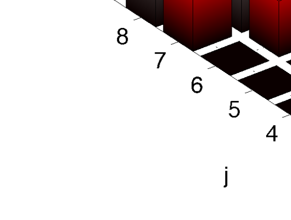
(c) Empirical with mask

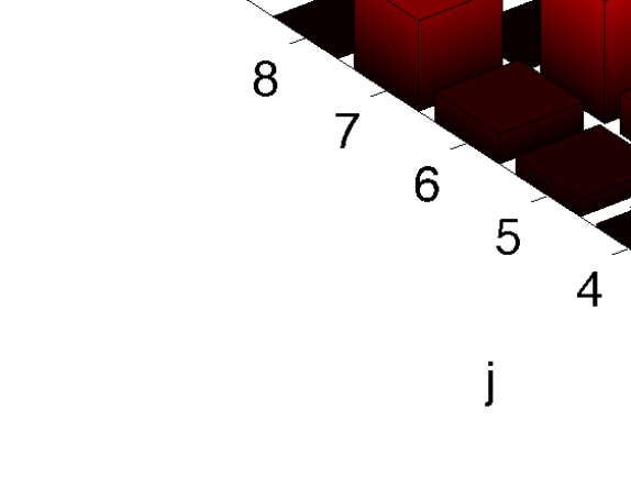
(d) Difference between analytic and empirical

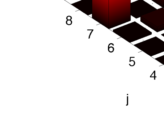
(e) Difference between empirical masked and unmasked

Figure 8: Correlation $\xi^{(jj^{\prime})}(\mathbf{\rho},\mathbf{\rho})$ computed analytically and empirically (from Monte Carlo simulations) in the absence and presence of a mask (${L}=256,\ {\lambda}=2,\ {N}=3)$.

Appendix A Auxiliary results

In this appendix we collect some useful technical results. In the first subsection we recall well-known results related to spherical harmonics, spin spherical harmonics, Wigner $D$-functions and some related properties. The latter subsections include results pivotal for the exhaustive proofs of the localisation of the directional scale-discretised wavelets $\Psi^{(j)}$ and the upper bound of the covariance between $W^{\Psi^{(j)}}(\rho_{1})$ and $W^{\Psi^{(j^{\prime})}}(\rho_{2})$. This appendix should be read in conjunction with the main text, where symbols and expressions introduced already are defined explicitly.

A.1 Spherical harmonics and Wigner $D$-functions

We succinctly recall the main definitions and properties of the spherical harmonic functions and the Wigner $D$-functions, which we make use of throughout the article. For further details and proofs we refer the reader to [35, 74].

The scalar spherical harmonic functions are explicitly defined by

$$Y_{\ell m}({\theta,\varphi})=(-1)^{m}\sqrt{\frac{2\ell+1}{4\pi}\frac{(\ell-m)!}{(\ell+m)!}}\>P_{\ell}^{m}({\cos\theta})\>{\rm exp}{({\rm i}m\varphi)}\>,$$ (79)

for natural $\ell\in\mathbb{N}$ and integer $m\in\mathbb{Z}$, $|m|\leq\ell$, where $P_{\ell}^{m}({\cdot})$ are the associated Legendre functions, which can be related to the Legendre polynomials $P_{{\ell}}({\cdot})$ by

$$P_{\ell}^{m}({\cos\theta})\equiv(\sin\theta)^{m}\frac{\mathrm{\,d}^{m}}{\mathrm{\,d}(\cos\theta)^{m}}P_{{\ell}}({\cos\theta})\>.$$ (80)

Recall the definition of the $C^{\infty}$ differential operator $\mathcal{T}_{m}$ specified by Eq. (37): it can be readily noted that

$$P_{\ell}^{m}(\cos\theta)=\mathcal{T}_{m}P_{\ell}(\cos\theta).$$ (81)

Note that here we adopt the Condon-Shortley phase convention, with the $(-1)^{m}$ phase factor included in Eq. (79) above. The orthogonality and completeness relations for the spherical harmonics read, respectively,

$$\langle{Y_{\ell m}},\>{Y_{\ell^{\prime}m^{\prime}}}\rangle=\int_{\mathbb{S}^{2}}\mathrm{\,d}\Omega(\theta,\varphi)\>Y_{\ell m}({\theta,\varphi})\>Y_{\ell^{\prime}m^{\prime}}^{\ast}({\theta,\varphi})=\delta_{{\ell}{\ell^{\prime}}}\delta_{{m}{m^{\prime}}}$$ (82)

and

$$\sum_{\ell=0}^{\infty}\sum_{m=-\ell}^{\ell}Y_{\ell m}({\theta,\varphi})\>Y_{\ell m}^{\ast}({\theta^{\prime},\varphi^{\prime}})=\delta(\cos\theta-\cos\theta^{\prime})\>\delta(\varphi-\varphi^{\prime})\>,$$ (83)

where $\delta_{{i}{j}}$ is the Kronecker delta symbol and $\delta(x)$ is the one-dimensional Dirac delta function.

The Wigner $D$-function $D_{mn}^{\ell}$, for integer $m,n\in\mathbb{Z}$, $|m|,|n|\leq\ell$, may be decomposed, in terms of Euler angles, by

$$D_{mn}^{\ell}(\alpha,\beta,\gamma)={\rm e}^{-{\rm i}m\alpha}\>d_{mn}^{\ell}(\beta)\>{\rm e}^{-{\rm i}n\gamma}\>.$$ (84)

The orthogonality and completeness relations for the Wigner $D$-functions read, respectively,

$$\langle{D_{mn}^{\ell}},\>{D_{m^{\prime}n^{\prime}}^{\ell^{\prime}}}\rangle=\int_{\mathrm{SO}(3)}\mathrm{\,d}\varrho(\mathbf{\rho})\>D_{mn}^{\ell}(\mathbf{\rho})\>D_{m^{\prime}n^{\prime}}^{\ell^{\prime}\ast}(\mathbf{\rho})=\frac{8\pi^{2}}{2\ell+1}\delta_{{\ell}{\ell^{\prime}}}\delta_{{m}{m^{\prime}}}\delta_{{n}{n^{\prime}}}\>,$$ (85)

and

$$\sum_{\ell=0}^{\infty}\sum_{m=-\ell}^{\ell}\sum_{n=-\ell}^{\ell}D_{mn}^{\ell}(\alpha,\beta,\gamma)\>D_{mn}^{\ell\ast}(\alpha^{\prime},\beta^{\prime},\gamma^{\prime})=\delta(\alpha-\alpha^{\prime})\>\delta(\cos\beta-\cos\beta^{\prime})\>\delta(\gamma-\gamma^{\prime})\>.$$ (86)

where $\langle{\cdot},\>{\cdot}\rangle$ is used to denote inner products over both the sphere and the rotation group (the case adopted can be inferred from the context).

We note the additive property of the $D$-functions is given by

$$D_{mn}^{\ell}(\alpha,\beta,\gamma)=\sum_{k=-\ell}^{\ell}D_{mk}^{\ell}(\alpha_{1},\beta_{1},\gamma_{1})\>D_{kn}^{\ell}(\alpha_{2},\beta_{2},\gamma_{2})\>,$$ (87)

where $\mathbf{\rho}=(\alpha,\beta,\gamma)$ describes the rotation formed by composing the rotations described by $\mathbf{\rho}_{1}=(\alpha_{1},\beta_{1},\gamma_{1})$ and $\mathbf{\rho}_{2}=(\alpha_{2},\beta_{2},\gamma_{2})$, i.e. $\mathbf{R}_{\mathbf{\rho}}=\mathbf{R}_{\mathbf{\rho}_{1}}\mathbf{R}_{\mathbf{\rho}_{2}}$. The Euler angles may be related explicitly by

$$\cot(\alpha-\alpha_{2})=\cos\beta_{2}\cot(\alpha_{1}+\gamma_{2})+\cot\beta_{1}\frac{\sin\beta_{2}}{\sin(\alpha_{1}+\gamma_{2})}\>,$$ (88)

$$\cos\beta=\cos\beta_{1}\cos\beta_{2}-\sin\beta_{1}\sin\beta_{2}\cos(\alpha_{1}+\gamma_{2}),$$ (89)

and

$$\cot(\gamma-\gamma_{1})=\cos\beta_{1}\cot(\alpha_{1}+\gamma_{2})+\cot\beta_{2}\frac{\sin\beta_{1}}{\sin(\alpha_{1}+\gamma_{2})}\>.$$ (90)

Thus

$$\sum_{k=-\ell}^{\ell}D_{km}^{\ell\ast}(\alpha_{1},\beta_{1},\gamma_{1})\>D_{kn}^{\ell}(\alpha_{2},\beta_{2},\gamma_{2})=D_{mn}^{\ell}(\alpha,\beta,\gamma)\>,$$ (91)

where now $\mathbf{\rho}=(\alpha,\beta,\gamma)$ describes the rotation formed by composing the inverse of the rotation described by $\mathbf{\rho}_{1}=(\alpha_{1},\beta_{1},\gamma_{1})$ and the rotation described by $\mathbf{\rho}_{2}=(\alpha_{2},\beta_{2},\gamma_{2})$, i.e. $\mathbf{R}_{\mathbf{\rho}}=\mathbf{R}_{\mathbf{\rho}_{1}}^{-1}\mathbf{R}_{\mathbf{\rho}_{2}}$, since

$$D_{mn}^{\ell}(\alpha,\beta,\gamma)=D_{nm}^{\ell\ast}(-\gamma,-\beta,-\alpha)\>.$$ (92)

For the case $\mathbf{\rho}_{1}=\mathbf{\rho}_{2}$,

$$\sum_{k=-\ell}^{\ell}D_{km}^{\ell\ast}(\alpha_{1},\beta_{1},\gamma_{1})\>D_{kn}^{\ell}(\alpha_{1},\beta_{1},\gamma_{1})=\delta_{{m}{n}}\>.$$ (93)

Finally, we note that one can relate the Wigner $D$-functions and the spherical harmonics (for further details and discussion we refer to [35, 57]):

$$Y_{\ell m}\left(\theta,\phi\right)=\sqrt{\frac{2\ell+1}{4\pi}}D_{m0}^{\ell\>\ast}(\varphi,\theta,0).$$ (94)

The Wigner $D$-functions may also be related to the spin spherical harmonics [57], ${{}_{n}Y_{\ell m}}\in\mathrm{L}^{2}({\mathbb{S}^{2}})$, which can be constructed from the scalar harmonics through repeated action of the differential spin raising/lowering operators. When applied to a spin-$n$ function, the spin raising and lowering operators are defined by

$$\eth\equiv-\sin^{n}\theta\biggl{(}\frac{\partial}{\partial\theta}+\frac{{\rm i}}{\sin\theta}\frac{\partial}{\partial\varphi}\biggr{)}\sin^{-n}\theta$$ (95)

and

$$\bar{\eth}\equiv-\sin^{-n}\theta\biggl{(}\frac{\partial}{\partial\theta}-\frac{{\rm i}}{\sin\theta}\frac{\partial}{\partial\varphi}\biggr{)}\sin^{n}\theta\>,$$ (96)

respectively. The spin-$n$ spherical harmonics can hence be expressed in terms of the scalar (spin-zero) harmonics by

$${{}_{n}Y_{\ell m}({\theta,\varphi})}=\biggl{[}\frac{(\ell-n)!}{(\ell+n)!}\biggr{]}^{1/2}\eth^{n}Y_{\ell m}({\theta,\varphi})\>,$$ (97)

for $0\leq n\leq\ell$, and by

$${{}_{n}Y_{\ell m}({\theta,\varphi})}=(-1)^{n}\biggl{[}\frac{(\ell+n)!}{(\ell-n)!}\biggr{]}^{1/2}\bar{\eth}^{-n}Y_{\ell m}({\theta,\varphi})\>,$$ (98)

for $-\ell\leq n\leq 0$. Spin spherical harmonics are related to the Wigner $D$-functions by [26]

$${{}_{n}Y_{\ell m}({\theta,\varphi})}=(-1)^{n}\sqrt{\frac{2\ell+1}{4\pi}}\>D_{m,-n}^{\ell\>\ast}(\varphi,\theta,0)\>.$$ (99)

Expressing the spin harmonics as spin raised or lower scalar harmonics, it follows that

$$D_{mn}^{\ell}(\alpha,\beta,\gamma)=\sqrt{\frac{4\pi}{2\ell+1}}\>\biggl{[}\frac{(\ell-n)!}{(\ell+n)!}\biggr{]}^{1/2}\bar{\eth}^{n}Y_{\ell m}^{\ast}({\beta,\alpha})\>{\rm exp}{({\rm i}n\gamma)}\>,$$ (100)

for $0\leq n\leq\ell$, and

$$D_{mn}^{\ell}(\alpha,\beta,\gamma)=(-1)^{n}\sqrt{\frac{4\pi}{2\ell+1}}\>\biggl{[}\frac{(\ell+n)!}{(\ell-n)!}\biggr{]}^{1/2}\eth^{-n}Y_{\ell m}^{\ast}({\beta,\alpha})\>{\rm exp}{({\rm i}n\gamma)}\>,$$ (101)

for $-\ell\leq n\leq 0$.

Before concluding this subsection, let us introduce the Mehler-Dirichlet approximation for Legendre polynomials. Further details can be found in [55]. Let us start from Eq. (32) in [18, p. 177], oncerning the integral representation of the Gegenbauer polynomials: as well-known in the literature, Legendre polynomials correspond to Gegenbauer of parameter $\frac{1}{2}$, so that we obtain

$$P_{\ell}(\cos\theta)=C_{\ell}^{\frac{1}{2}}(\cos\theta)=\frac{\sqrt{2}\Gamma(1)\Gamma(\ell+1)}{\pi^{\frac{1}{2}}\ell!\Gamma(\frac{1}{2})\Gamma(1)}\int_{0}^{\theta}\frac{\cos(\ell+\frac{1}{2})\phi}{\sqrt{\cos\phi-\cos\theta}}\mathrm{\,d}\phi=\frac{\sqrt{2}}{\pi}\int_{0}^{\theta}\frac{\cos(\ell+\frac{1}{2})\phi}{\sqrt{\cos\phi-\cos\theta}}\mathrm{\,d}\phi\>.$$ (102)

As suggested in [18], we replace $\phi$ and $\theta$ with $\pi-\phi$ and $\pi-\theta$ respectively, to get

$$P_{\ell}(\cos(\pi-\theta))=\frac{\sqrt{2}}{\pi}\int_{\phi}^{\pi}\frac{\cos\bigl{(}(\ell+\frac{1}{2})\pi-\ell(\phi+\frac{1}{2})\bigr{)}}{\sqrt{\cos\theta-\cos\phi}}\mathrm{\,d}\phi\>.$$ (103)

On one hand, recall that

$$\cos\Bigl{(}\Bigl{(}\ell+\frac{1}{2}\Bigr{)}\pi-\ell\Bigl{(}\phi+\frac{1}{2}\Bigr{)}\Bigr{)}=(-1)^{\ell}\sin\Bigl{(}\ell\Bigl{(}\phi+\frac{1}{2}\Bigr{)}\Bigr{)}\>.$$ (104)

On the other hand, using the symmetry property of Legendre polynomials, we have

$$P_{\ell}\bigl{(}\cos(\pi-\theta)\bigr{)}=P_{\ell}(-\cos(\theta))=(-1)^{\ell}P_{\ell}(\cos(\theta))\>.$$ (105)

Combining together all these results, we obtain

$$P_{\ell}(\cos(\theta))=\frac{\sqrt{2}}{\pi}\int_{\phi}^{\pi}\frac{\sin(\ell(\phi+\frac{1}{2}))}{\sqrt{\cos\theta-\cos\phi}}\mathrm{\,d}\phi\>.$$ (106)

A.2 A general result on localisation over compact manifolds

Here we recall the general result established in [25] as Theorem 2.2, properly adapted to the sphere ${\mathbb{S}^{2}}$. Let $g\in C^{\infty}(\mathbb{R})$ and let $\left\{\lambda_{\ell}\right\}$ be the set of eigenvalues associated to the Beltrami-Laplacian operator over ${\mathbb{S}^{2}}$. Let $\Lambda(x,y,t;g)$ be given by

$$\Lambda(\omega_{1},\omega_{2},t;g)\equiv\sum_{\ell=0}^{\infty}\sum_{m=-\ell}^{\ell}g(t\sqrt{\lambda_{\ell}})\>Y_{\ell m}(\omega_{1})\>{Y}_{\ell m}^{\ast}(\omega_{2})\>.$$ (107)

For $t\in\mathbb{R}^{+}_{\ast}$, for any function $g\in C^{\infty}(\mathbb{R})$, for every pair of differential operators on the unit sphere $\mathbb{S}^{2}$, $T_{1}$ and $T_{2}$, depending respectively on $\omega_{1}\in{\mathbb{S}^{2}}$ and $\omega_{2}\in{\mathbb{S}^{2}}$, and defined such that $\deg T_{1}=i_{1}$, $\deg T_{2}=i_{2}$, and for every non-negative integer $\tau\in\mathbb{N}$, there exists a constant $C_{\tau}\in\mathbb{R}^{+}_{\ast}$ such that

$$\bigl{|}T_{1}\>T_{2}\>\Lambda(\omega_{1},\omega_{2},t;g)\bigr{|}\leq\frac{C_{\tau}\>t^{-2-i_{1}-i_{2}}}{\Bigl{(}1+\frac{d(\omega_{1},\omega_{2})}{t}\Bigr{)}^{\tau}}\text{ , for all }t\in\mathbb{R}^{+}_{\ast},\text{ }\omega_{1},\omega_{2}\in{\mathbb{S}^{2}}\>,$$ (108)

where $d(\omega_{1},\omega_{2})=\arccos(\mbox{\boldmath${\hat{\omega}_{1}}$}\cdot\mbox{\boldmath${\hat{\omega}_{2}}$})$ denotes the geodesic distance between $\omega_{1},\omega_{2}\in{\mathbb{S}^{2}}$. In the framework of directional wavelets, we have:

$$\Lambda^{(j)}(x,y)\equiv\Lambda(x,y,\lambda^{j}L^{-1};\kappa^{(j)}(\ell))\>.$$ (109)

A.3 Upper bound of $\sqrt{(\ell-m)!/(\ell+m)!}$

As far as the behaviour of $\sqrt{(\ell-m)!/(\ell+m)!}$ is concerned, we make use of the following approximation, which we show here:

$$\sqrt{\frac{(\ell-m)!}{(\ell+m)!}}\leq\ell^{-m}\>.$$ (110)

Stirling’s approximation leads to

$$\frac{(\ell-m)!}{(\ell+m)!} \approx\frac{(\ell-m)^{\frac{1}{2}}(\ell-m)^{\ell-m}{\rm exp}{(-(\ell-m)}}{(\ell+m)^{\frac{1}{2}}(\ell+m)^{\ell+m}{\rm exp}{(-(\ell+m))}}$$ (111)

$$=\ell^{-2m}{\rm exp}{(2m)}\Biggl{(}\frac{(1-\frac{m}{\ell})}{(1+\frac{m}{\ell})}\Biggr{)}^{\ell}\frac{(1-\frac{m}{\ell})^{\frac{1}{2}-m}}{(1+\frac{m}{\ell})^{{}^{\frac{1}{2}+m}}}\>.$$ (112)

Consider now the positive function $h\in C^{\infty}$, defined on the support $(-1,1)$ as

$$h(x)=\biggl{(}\frac{1-x}{1+x}\biggr{)}^{\frac{1}{2}}\frac{1}{(1-x^{2})^{{}^{m}}}\>.$$ (113)

Its first derivative is given by $\frac{\mathrm{\,d}}{\mathrm{\,d}x}h(x)=(1+x)^{-(m+\frac{3}{2})}(1-x)^{{}^{-(m+\frac{1}{2})}}(2mx-1)$, so that we have $\frac{\mathrm{\,d}}{\mathrm{\,d}x}h(x)=0$ for $x=(2m)^{-1}$. The function $h$ is therefore monotonically decreasing in the interval $(-1,1/2m)$ and increasing for $x\in(1/2m,1)\,$. Consider $x\equiv m/\ell$: because $m=-M,...,M$, it follows that $|m/\ell|\leq|M/\ell|$. Hence we obtain

$$\biggl{|}\frac{M}{\ell}\biggr{|}<1\Rightarrow\biggl{|}1\pm\frac{m}{\ell}\biggr{|}>0\>.$$ (114)

Therefore, we have that, for any $\ell$,

$$h\Bigl{(}\frac{m}{\ell}\Bigr{)}<+\infty\>.$$ (115)

On the other hand, $h$ attains its minimum for $\ell=2m^{2}$, where

$$h\biggl{(}\frac{1}{2m}\biggr{)}=\biggl{(}\frac{2m-1}{2m+1}\biggr{)}^{\frac{1}{2}}\biggl{(}\frac{4m^{2}}{4m^{2}-1}\biggr{)}>0\>.$$ (116)

Because $\ell>(L\lambda^{-(1+j)}\vee m)$ and $\lim_{\ell\rightarrow\infty}h(\frac{m}{\ell})=1$, we have that

$$\frac{(1-\frac{m}{\ell})^{\frac{1}{2}-m}}{(1+\frac{m}{\ell})^{{}^{\frac{1}{2}+m}}}\leq\max\biggl{(}1,h\biggl{(}\frac{m}{(L\lambda^{-(1+j)}\vee m)}\biggr{)}\biggr{)}\>.$$ (117)

Furthermore, for large $\ell$, it can be easily seen that

$$\lim_{\ell\rightarrow+\infty}\frac{(1-\frac{m}{\ell})^{\ell}}{(1+\frac{m}{\ell})^{\ell}}={\rm exp}{(-2m)}\>.$$ (118)

Consequently, the approximation specified above holds for large $\ell$. On the other hand, for small $\ell$, let us define $F_{\ell,m}={\rm exp}{(}{2m})\frac{(1-\frac{m}{\ell})^{\ell}}{(1+\frac{m}{\ell})^{\ell}}$. We must prove that $F_{\ell,m}\leq 1$. Let us compute

$$\log F_{\ell,m}=2m+\ell\Bigl{(}\log\Bigl{(}1-\frac{m}{\ell}\Bigr{)}-\log(1+\frac{m}{\ell}\Bigr{)}\Bigr{)}\>.$$ (119)

Now, because $\log(1+x)=x-\frac{x^{2}}{2}+\frac{x^{3}}{3}+\mathcal{O}(x^{4})$ and $\log(1-x)=-x-\frac{x^{2}}{2}-\frac{x^{3}}{3}+\mathcal{O}(x^{4})$, we have

$$\log F_{\ell,m}=2m+\ell\biggl{(}-\frac{m}{\ell}-\frac{1}{2}\frac{m^{2}}{\ell^{2}}-\frac{1}{3}\frac{m^{3}}{\ell^{3}}-\frac{m}{\ell}+\frac{1}{2}\frac{m^{2}}{\ell^{2}}-\frac{1}{3}\frac{m^{3}}{\ell^{3}}+\mathcal{O}\Bigl{(}\Bigl{(}\frac{m}{\ell}\Bigr{)}^{4}\Bigr{)}\biggr{)},$$ (120)

so that

$$\log F_{\ell,m}=-\frac{2}{3}\frac{m^{3}}{\ell^{2}}+\mathcal{O}\Bigl{(}\frac{m^{4}}{\ell^{3}}\Bigr{)}\leq 0.$$ (121)

Thus, $F_{\ell,m}\leq 1$, and consequently the approximation specified above also holds for small $\ell$.

A.4 Upper bound of $U^{(j)}_{m}(\cos\theta)$

As far as the kernel $U^{(j)}_{m}(\cos\theta)$, defined in Eq. (43), is concerned, we obtain the following upper bound: there exists $\xi\in\mathbb{R^{+}}$ such that

$$\bigl{|}U^{(j)}_{m}(\cos\theta)\bigr{|}\leq\frac{C_{\xi}/\varepsilon_{j}^{2}}{\Bigl{(}1+\bigl{|}\frac{\theta}{\varepsilon_{j}}\bigl{|}\Bigr{)}^{\xi}}\>.$$ (122)

The construction of this bound strictly follows the procedure used to establish the localisation property for the so-called spherical standard needlets developed in [55]. First of all, observe that for large $\ell$, $b_{m,\varepsilon_{j}}\left(\varepsilon_{j}\left(\ell+\frac{1}{2}\right)\right)\equiv b_{m,\varepsilon_{j}}\left(\varepsilon_{j}\left(\ell\right)\right)$. Furthermore, using the Meher-Dirichlet formula for Legendre polynomials Eq. (106), we obtain

$$U^{(j)}_{m}(\cos\theta) \leq\sum_{\ell=0}^{\infty}b_{m,\varepsilon_{j}}\Bigl{(}\ell+\frac{1}{2}\Bigr{)}\Bigl{(}\ell+\frac{1}{2}\Bigr{)}P_{\ell}(\cos\theta)$$ (123)

$$=\frac{1}{2}\int_{\theta}^{\pi}\frac{G_{m,\varepsilon_{j}}(\alpha)}{\sqrt{\cos\theta-\cos\alpha}}d\alpha\>,$$ (124)

where

$$G_{m,\varepsilon_{j}}(\alpha)=\sum_{\ell=-\infty}^{\infty}b_{m,\varepsilon_{j}}\Bigl{(}\ell+\frac{1}{2}\Bigr{)}\Bigl{(}\ell+\frac{1}{2}\Bigr{)}\sin\Bigl{(}\alpha\Bigl{(}\ell+\frac{1}{2}\Bigr{)}\Bigr{)}\>.$$ (125)

Observe that $b_{m,\varepsilon_{j}}(x)x\sin(\alpha x)$ is an even function. We now compute the Fourier transform, here denoted $\mathcal{F}[\cdot]$, of $G_{m,\varepsilon_{j}}(\alpha)$, considering three different cases depending on the sign of $m$:

1. $m=0$. In this case, the proof is trivially equivalent to [55].

2. $m<0$. In this case, we have

   $$xb_{m,\varepsilon}(x)=\kappa^{(j)}(x)(x)^{|m|+1}=\kappa_{\lambda}(\varepsilon_{j}x)(x)^{|m|+1}\>.$$ (126)

   For any integrable function $g$, let its Fourier transform be denoted by $\mathcal{F}\left[f\left(x\right)\right]\left(\nu\right)$, $\nu\in\mathbb{R}$. Furthermore we define $\widehat{\kappa}\left(\nu\right)=\mathcal{F}\left[\kappa_{\lambda}\left(x\right)\right]\left(\nu\right)$. Therefore, we obtain

   $$\mathcal{F}[xb_{m}(\varepsilon_{j}x)](\nu) =\mathcal{F}[x^{|m|+1}\kappa_{\lambda}(\varepsilon_{j}x)](\nu)$$ (127)

   $$=\frac{i^{|m|+1}}{\varepsilon_{j}}\widehat{\kappa}^{(|m|+1)}\Bigl{(}\frac{\nu}{\varepsilon_{j}}\Bigr{)}\>,$$ (128)

   where we adopt the notation here $\widehat{\kappa}^{(|m|+1)}(\cdot)=\frac{d^{|m|+1}}{d\nu^{|m|+1}}\mathcal{F}[\kappa_{\lambda}(x)](\cdot)$. Hence, we have

   $$\int_{\mathbb{R}}b_{m,\varepsilon}\Bigl{(}x+\frac{1}{2}\Bigr{)}\Bigl{(}x+\frac{1}{2}\Bigr{)}\sin\Bigl{(}\theta\Bigl{(}x+\frac{1}{2}\Bigr{)}\Bigr{)}{\rm exp}{(-{\rm i}\nu x)}\mathrm{\,d}x=\frac{1}{2\pi i}{\rm exp}{\Bigl{(}{\rm i}\frac{\nu}{2}\Bigr{)}}\frac{i^{|m|+1}}{\varepsilon_{j}}\widehat{\kappa}^{(|m|+1)}\Bigl{(}\frac{\nu}{\varepsilon_{j}}\Bigr{)}\>,$$ (129)

   which, by Poisson summation formula and some simplifications, leads to

   $$G_{m,\varepsilon_{j}}(\cos\theta)\leq\frac{1}{2\pi\varepsilon}\biggl{|}\sum_{\nu=-\infty}^{+\infty}\widehat{\kappa}^{(|m|+1)}\biggl{(}\frac{\theta+\nu}{\varepsilon_{j}}\biggr{)}\biggr{|}\>.$$ (130)

   Now, following [55], standard Fourier properties yield

   $$\mathcal{F}\biggl{[}\frac{\mathrm{\,d}^{r}}{\mathrm{\,d}x^{r}}\bigl{(}x^{1+|m|}\kappa_{\lambda}(x)\bigr{)}\biggr{]}(\nu)=i^{r+1}\nu^{r}\widehat{\kappa}^{(|m|+1)}(\nu)\>.$$ (131)

   Hence, we obtain

   $$\biggl{|}\frac{\theta+\nu}{\varepsilon_{j}}\biggr{|}^{r}\biggl{|}\widehat{\kappa}^{(|m|+1)}\Bigl{(}\frac{\phi+\nu}{\varepsilon_{j}}\Bigr{)}\biggr{|}\leq\frac{1}{\varepsilon_{j}}\biggl{\|}\frac{\mathrm{\,d}^{r}}{\mathrm{\,d}x^{r}}\bigl{(}x^{1+|m|}\kappa_{\lambda}(x)\bigr{)}\biggr{\|}_{L^{1}}\>.$$ (132)

   Therefore, for any given $\xi>M$, if

   $$V_{\xi,\kappa_{\lambda}}\equiv\max_{0\leq r\leq\xi}\biggl{\|}\frac{\mathrm{\,d}^{r}}{\mathrm{\,d}x^{r}}\bigl{(}x^{1+|m|}\kappa_{\lambda}(x)\bigr{)}\biggr{\|}_{L^{1}}\>,$$ (133)

   we have

   $$G_{m,\varepsilon_{j}}(\theta)\leq\frac{1}{4\pi^{2}\varepsilon_{j}}\biggl{|}\sum_{\nu=-\infty}^{+\infty}\frac{2V_{\xi,\kappa_{\lambda}}/\varepsilon_{j}}{1+\bigl{|}\frac{\theta+\nu}{\varepsilon_{j}}\bigr{|}^{\xi}}\biggr{|}\>.$$ (134)

   The remainder of the proof is equivalent to [55].

3. $m>0$. By construction,  $b_{m,\varepsilon_{j}}(\cdot)$ fulfils all the conditions necessary for boundedness as in [55].

In all the three cases, we have therefore

$$\bigl{|}U^{(j)}_{m}(\cos\theta)\bigr{|}\leq\frac{V_{\xi,\kappa_{\lambda}}}{4\pi^{2}\varepsilon_{j}^{2}}\int_{\theta}^{\pi}\frac{1}{1+\bigl{|}\frac{\phi}{\varepsilon_{j}}\bigr{|}^{\xi}}\frac{d\phi}{\sqrt{\cos\theta-\cos\phi}}\>.$$ (135)

According to [55], we obtain

$$\bigl{|}U^{(j)}_{m}(\cos\theta)\bigr{|}\leq\frac{C_{\xi}/\varepsilon_{j}^{2}}{(1+\bigl{|}\frac{\theta}{\varepsilon_{j}}\bigr{|})^{\xi}}\>.$$ (136)

References

- Antoine et al. [2002] Antoine, J.-P., Demanet, L., Jacques, L., Vandergheynst, P., 2002. Wavelets on the sphere: implementation and approximations. Applied Comput. Harm. Anal. 13 (3), 177–200.
- Antoine and Vandergheynst [1998] Antoine, J.-P., Vandergheynst, P., 1998. Wavelets on the n-sphere and related manifolds. J. Math. Phys. 39 (8), 3987–4008.
- Antoine and Vandergheynst [1999] Antoine, J.-P., Vandergheynst, P., 1999. Wavelets on the 2-sphere: a group theoretical approach. Applied Comput. Harm. Anal. 7, 1–30.
- Audet [2011] Audet, P., 2011. Directional wavelet analysis on the sphere: Application to gravity and topography of the terrestrial planets. J. Geophys. Res. 116 (E1).
- Audet [2014] Audet, P., 2014. Toward mapping the effective elastic thickness of planetary lithospheres from a spherical wavelet analysis of gravity and topography. Phys. Earth Planet In. 226 (0), 48–82.
- Baldi et al. [2009] Baldi, P., Kerkyacharian, G., Marinucci, D., Picard, D., 2009. Asymptotics for spherical needlets. Ann. Stat. 37 No.3, 1150–1171.
- Barreiro et al. [2000] Barreiro, R. B., Hobson, M. P., Lasenby, A. N., Banday, A. J., Górski, K. M., Hinshaw, G., 2000. Testing the Gaussianity of the COBE-DMR data with spherical wavelets. Mon. Not. Roy. Astron. Soc. 318, 475–481.
- Bennett et al. [2013] Bennett, C. L., Larson, D., Weiland, J. L., Jarosik, N., Hinshaw, G., Odegard, N., Smith, K. M., Hill, R. S., Gold, B., Halpern, M., Komatsu, E., Nolta, M. R., Page, L., Spergel, D. N., Wollack, E., Dunkley, J., Kogut, A., Limon, M., Meyer, S. S., Tucker, G. S., Wright, E. L., Oct. 2013. Nine-year Wilkinson Microwave Anisotropy Probe (WMAP) Observations: Final Maps and Results. Astrophys. J. Supp. 208, 20.
- Bobin et al. [2013] Bobin, J., Starck, J.-L., Sureau, F., Basak, S., Feb. 2013. Sparse component separation for accurate cosmic microwave background estimation. Astron. & Astrophys. 550, A73.
- Bogdanova et al. [2004] Bogdanova, I., Vandergheynst, P., Antoine, J.-P., Jacques, L., Morvidone, M., Sept 2004. Discrete wavelet frames on the sphere. In: Signal Processing Conference, 2004 12th European. pp. 49–52.
- Bogdanova et al. [2005] Bogdanova, I., Vandergheynst, P., Antoine, J.-P., Jacques, L., Morvidone, M., 2005. Stereographic wavelet frames on the sphere. Applied Comput. Harm. Anal. 19 (2), 223–252.
- Bond and Efstathiou [1987] Bond, J. R., Efstathiou, G., Jun. 1987. The statistics of cosmic background radiation fluctuations. Mon. Not. Roy. Astron. Soc. 226, 655–687.
- Charléty et al. [2012] Charléty, J., Nolet, G., Voronin, S., Loris, I., Simons, F. J., Daubechies, I., Sigloch, K., 2012. Inversion with a sparsity constraint: application to mantle tomography. In: EGU General Assembly Conference Abstracts. EGU General Assembly Conference Abstracts.
- Dahlke and Maass [1996] Dahlke, S., Maass, P., 1996. Continuous wavelet transforms with applications to analyzing functions on sphere. J. Fourier Anal. and Appl. 2, 379–396.
- Delabrouille et al. [2009] Delabrouille, J., Cardoso, J.-F., Le Jeune, M., Betoule, M., Fay, G., Guilloux, F., Jan. 2009. A full sky, low foreground, high resolution CMB map from WMAP. Astron. & Astrophys. 493, 835–857.
- Dodelson [2003] Dodelson, S., 2003. Modern Cosmology. Academic Press. Academic Press.
- Durastanti et al. [2014] Durastanti, C., Fantaye, Y., Hansen, F., Marinucci, D., Pesenson, I. Z., Nov. 2014. Simple proposal for radial 3D needlets. Phys. Rev. D. 90 (10), 103532.
- Erdélyi et al. [1981] Erdélyi, A., Magnus, W.; Oberhettinger, F., Tricomi, F. G., 1981. Higher Trascendental Functions, Vol. 2. New York Krieger.
- Freeden and Windheuser [1997] Freeden, W., Windheuser, U., 1997. Combined spherical harmonic and wavelet expansion – a future concept in the Earth’s gravitational determination. Applied Comput. Harm. Anal. 4, 1–37.
- Freeman and Adelson [1991] Freeman, W., Adelson, E., 1991. The design and use of steerable filters. IEEE Trans. Pattern Anal. 13 (9), 891–906.
- Geller et al. [2008] Geller, D., Hansen, F. K., Marinucci, D., Kerkyacharian, G., Picard, D., 2008. Spin needlets for cosmic microwave background polarization data analysis. Phys. Rev. D. 78 (12), 123533–+.
- Geller et al. [2009] Geller, D., Lan, X., Marinucci, D., Jul. 2009. Spin Needlets Spectral Estimation. Electron. J. Statist. 3, 1497–1530.
- Geller and Marinucci [2010] Geller, D., Marinucci, D., Nov. 2010. Spin Wavelets on the Sphere. J. Fourier Anal. and Appl. 16 (6), 840––884.
- Geller and Marinucci [2011] Geller, D., Marinucci, D., Jun. 2011. Mixed Needlets. J. Math. Anal. Appl. 375 (2), 610––630.
- Geller and Mayeli [2009] Geller, D., Mayeli, A., Jun. 2009. Nearly Tight Frames and Space-Frequency Analysis on Compact Manifolds. Math. Z. 263, 235–264.
- Goldberg et al. [1967] Goldberg, J. N., Macfarlane, A. J., Newman, E. T., Rohrlich, F., Sudarshan, E. C. G., 1967. Spin- spherical harmonics and . J. Math. Phys. 8 (11), 2155–2161.
- Górski et al. [2005] Górski, K. M., Hivon, E., Banday, A. J., Wandelt, B. D., Hansen, F. K., Reinecke, M., Bartelmann, M., 2005. Healpix – a framework for high resolution discretization and fast analysis of data distributed on the sphere. Astrophys. J. 622, 759–771.
- Hinshaw et al. [2013] Hinshaw, G., Larson, D., Komatsu, E., Spergel, D. N., Bennett, C. L., Dunkley, J., Nolta, M. R., Halpern, M., Hill, R. S., Odegard, N., Page, L., Smith, K. M., Weiland, J. L., Gold, B., Jarosik, N., Kogut, A., Limon, M., Meyer, S. S., Tucker, G. S., Wollack, E., Wright, E. L., Oct. 2013. Nine-year Wilkinson Microwave Anisotropy Probe (WMAP) Observations: Cosmological Parameter Results. Astrophys. J. Supp. 208, 19.
- Holschneider [1996] Holschneider, M., 1996. Continuous wavelet transforms on the sphere. J. Math. Phys. 37, 4156–4165.
- Lan and Marinucci [2008] Lan, X., Marinucci, D., 2008. The needlets bispectrum. Electronic Journal of Statistics 2, 332–367.
- Lanusse et al. [2012] Lanusse, F., Rassat, A., Starck, J.-L., Apr. 2012. Spherical 3D isotropic wavelets. Astron. & Astrophys. 540, A92.
- Leistedt and McEwen [2012] Leistedt, B., McEwen, J. D., 2012. Exact wavelets on the ball. IEEE Trans. Sig. Proc. 60 (12), 6257–6269.
- Leistedt et al. [2013] Leistedt, B., McEwen, J. D., Vandergheynst, P., Wiaux, Y., 2013. S2LET: A code to perform fast wavelet analysis on the sphere. Astron. & Astrophys. 558 (A128), 1–9.
- Loris et al. [2010] Loris, I., Simons, F. J., Daubechies, I., Nolet, G., Fornasier, M., Vetter, P., Judd, S., Voronin, S., Vonesch, C., Charléty, J., May 2010. A new approach to global seismic tomography based on regularization by sparsity in a novel 3D spherical wavelet basis. In: EGU General Assembly Conference Abstracts. Vol. 12 of EGU General Assembly Conference Abstracts. p. 6033.
- Marinucci and Peccati [2011] Marinucci, D., Peccati, G., 2011. Random Fields on the Sphere: Representation, Limit Theorem and Cosmological Applications. Cambridge University Press.
- Marinucci et al. [2008] Marinucci, D., Pietrobon, D., Balbi, A., Baldi, P., Cabella, P., Kerkyacharian, G., Natoli, P., Picard, D., Vittorio, N., 2008. Spherical needlets for cosmic microwave background data analysis. Mon. Not. Roy. Astron. Soc. 383, 539–545.
- McEwen et al. [2014] McEwen, J. D., Büttner, M., Leistedt, B., Peiris, H. V., Vandergheynst, P., Wiaux, Y., 2014. On spin scale-discretised wavelets on the sphere for the analysis of CMB polarisation. In: Proceedings IAU Symposium No. 306, 2014.
- McEwen et al. [2015a] McEwen, J. D., Büttner, M., Leistedt, B., Peiris, H. V., Wiaux, Y., 2015a. A novel sampling theorem on the rotation group. IEEE Sig. Proc. Let., submitted.
- McEwen et al. [2006a] McEwen, J. D., Hobson, M. P., Lasenby, A. N., 2006a. A directional continuous wavelet transform on the sphere. ArXiv.
- McEwen et al. [2005] McEwen, J. D., Hobson, M. P., Lasenby, A. N., Mortlock, D. J., 2005. A high-significance detection of non-Gaussianity in the WMAP 1-year data using directional spherical wavelets. Mon. Not. Roy. Astron. Soc. 359, 1583–1596.
- McEwen et al. [2006b] McEwen, J. D., Hobson, M. P., Lasenby, A. N., Mortlock, D. J., 2006b. A high-significance detection of non-Gaussianity in the WMAP 3-year data using directional spherical wavelets. Mon. Not. Roy. Astron. Soc. 371, L50–L54.
- McEwen et al. [2006c] McEwen, J. D., Hobson, M. P., Lasenby, A. N., Mortlock, D. J., 2006c. Non-Gaussianity detections in the Bianchi VIIh corrected WMAP 1-year data made with directional spherical wavelets. Mon. Not. Roy. Astron. Soc. 369, 1858–1868.
- McEwen et al. [2008a] McEwen, J. D., Hobson, M. P., Lasenby, A. N., Mortlock, D. J., 2008a. A high-significance detection of non-Gaussianity in the WMAP 5-year data using directional spherical wavelets. Mon. Not. Roy. Astron. Soc. 388 (2), 659–662.
- McEwen et al. [2007a] McEwen, J. D., Hobson, M. P., Mortlock, D. J., Lasenby, A. N., 2007a. Fast directional continuous spherical wavelet transform algorithms. IEEE Trans. Sig. Proc. 55 (2), 520–529.
- McEwen and Leistedt [2013] McEwen, J. D., Leistedt, B., 2013. Fourier-Laguerre transform, convolution and wavelets on the ball. In: 10th International Conference on Sampling Theory and Applications (SampTA). pp. 329–333.
- McEwen et al. [2015b] McEwen, J. D., Leistedt, B., Büttner, M., Peiris, H. V., Wiaux, Y., 2015b. Directional spin wavelets on the sphere. IEEE Trans. Sig. Proc., submitted.
- McEwen and Scaife [2008] McEwen, J. D., Scaife, A. M. M., 2008. Simulating full-sky interferometric observations. Mon. Not. Roy. Astron. Soc. 389 (3), 1163–1178.
- McEwen et al. [2013] McEwen, J. D., Vandergheynst, P., Wiaux, Y., 2013. On the computation of directional scale-discretized wavelet transforms on the sphere. In: SPIE Wavelets and Sparsity XV. Vol. 8858.
- McEwen et al. [2007b] McEwen, J. D., Vielva, P., Hobson, M. P., Martínez-González, E., Lasenby, A. N., 2007b. Detection of the ISW effect and corresponding dark energy constraints made with directional spherical wavelets. Mon. Not. Roy. Astron. Soc. 373, 1211–1226.
- McEwen et al. [2007c] McEwen, J. D., Vielva, P., Wiaux., Y., Barreiro, R. B., Cayón, L., Hobson, M. P., Lasenby, A. N., Martínez-González, E., Sanz, J. L., 2007c. Cosmological applications of a wavelet analysis on the sphere. J. Fourier Anal. and Appl. 13 (4), 495–510.
- McEwen and Wiaux [2011] McEwen, J. D., Wiaux, Y., 2011. A novel sampling theorem on the sphere. IEEE Trans. Sig. Proc. 59 (12), 5876–5887.
- McEwen et al. [2011] McEwen, J. D., Wiaux, Y., Eyers, D. M., 2011. Data compression on the sphere. Astron. & Astrophys. 531, A98.
- McEwen et al. [2008b] McEwen, J. D., Wiaux, Y., Hobson, M. P., Vandergheynst, P., Lasenby, A. N., 2008b. Probing dark energy with steerable wavelets through correlation of WMAP and NVSS local morphological measures. Mon. Not. Roy. Astron. Soc. 384 (4), 1289–1300.
-
Mhaskar et al. [2000]
Mhaskar, H., Narcowich, F., Prestin, J., Ward, J., 2000. Polynomial frames on
the sphere. Advances in Computational Mathematics 13 (4), 387–403.
URL http://dx.doi.org/10.1023/A:1016639802349 - Narcowich et al. [2006] Narcowich, F. J., Petrushev, P., Ward, J. D., 2006. Localized tight frames on spheres. SIAM J. Math. Anal. 38 (2), 574–594.
- Narcowich and Ward [1996] Narcowich, F. J., Ward, J. D., 1996. Non-stationary wavelets on the m-sphere for scattered data. Applied Comput. Harm. Anal. 3, 324–336.
- Newman and Penrose [1966] Newman, E. T., Penrose, R., 1966. Note on the Bondi-Metzner-Sachs group. J. Math. Phys. 7 (5), 863–870.
- Pietrobon et al. [2010] Pietrobon, D., Balbi, A., Cabella, P., Gorski, K. M., Nov. 2010. NeedATool: A Needlet Analysis Tool for Cosmological Data Processing. Astrophys. J. 723, 1–9.
- Pietrobon et al. [2006] Pietrobon, D., Balbi, A., Marinucci, D., Aug. 2006. Integrated Sachs-Wolfe effect from the cross-correlation of WMAP 3-year and NVSS: new results and constraints on dark energy. Phys. Rev. D. 74 (4), 043524–+.
- Planck Collaboration XII [2014] Planck Collaboration XII, 2014. Planck 2013 results. XII. Diffuse component separation. Astron. & Astrophys. 571, A12.
- Planck Collaboration XXIII [2014] Planck Collaboration XXIII, 2014. Planck 2013 results. XXIII. Isotropy and statistics of the CMB. Astron. & Astrophys. 571 (A23).
- Planck Collaboration XXIV [2014] Planck Collaboration XXIV, 2014. Planck 2013 results. XXIV. Constraints on primordial non-Gaussianity. Astron. & Astrophys. 571, A24.
- Planck Collaboration XXV [2014] Planck Collaboration XXV, 2014. Planck 2013 results. XXV. Searches for cosmic strings and other topological defects. Astron. & Astrophys. 571 (A25).
- Potts and Tasche [1995] Potts, D., Tasche, M., 1995. Interpolatory wavelets on the sphere. In: Approximation Theory VIII. pp. 335–342.
- Sanz et al. [2006] Sanz, J. L., Herranz, D., López-Caniego, M., Argüeso, F., Sep. 2006. Wavelets on the sphere – application to the detection problem. In: EUSIPCO.
- Schmitt et al. [2010] Schmitt, J., Starck, J. L., Casandjian, J. M., Fadili, J., Grenier, I., Jul. 2010. Poisson denoising on the sphere: application to the Fermi gamma ray space telescope. Astron. & Astrophys. 517, A26.
- Schröder and Sweldens [1995] Schröder, P., Sweldens, W., 1995. Spherical wavelets: efficiently representing functions on the sphere. In: Computer Graphics Proceedings (SIGGRAPH ‘95). pp. 161–172.
- Simons et al. [2011] Simons, F. J., Loris, I., Brevdo, E., Daubechies, I. C., 2011. Wavelets and wavelet-like transforms on the sphere and their application to geophysical data inversion. In: SPIE Wavelets and Sparsity XIV.
- Simons et al. [2011] Simons, F. J., Loris, I., Nolet, G., Daubechies, I. C., Voronin, S., Judd, J. S., Vetter, P. A., Charléty, J., Vonesch, C., Nov. 2011. Solving or resolving global tomographic models with spherical wavelets, and the scale and sparsity of seismic heterogeneity. Geophysical Journal International 187, 969–988.
- Starck et al. [2009] Starck, J., Moudden, Y., Bobin, J., Apr. 2009. Polarized wavelets and curvelets on the sphere. Astron. & Astrophys. 497, 931–943.
- Starck et al. [2006] Starck, J.-L., Moudden, Y., Abrial, P., Nguyen, M., Feb. 2006. Wavelets, ridgelets and curvelets on the sphere. Astron. & Astrophys. 446, 1191–1204.
- Sweldens [1997] Sweldens, W., 1997. The lifting scheme: a construction of second generation wavelets. SIAM J. Math. Anal. 29 (2), 511–546.
- Torrésani [1995] Torrésani, B., 1995. Position-frequency analysis for signals defined on spheres. Signal Proc. 43, 341–346.
- Varshalovich et al. [1989] Varshalovich, D. A., Moskalev, A. N., Khersonskii, V. K., 1989. Quantum theory of angular momentum. World Scientific, Singapore.
- Vielva et al. [2004] Vielva, P., Martínez-González, E., Barreiro, R. B., Sanz, J. L., Cayón, L., 2004. Detection of non-Gaussianity in the WMAP 1-year data using spherical wavelets. Astrophys. J. 609, 22–34.
- Vielva et al. [2006a] Vielva, P., Martínez-González, E., Tucci, M., 2006a. Cross-correlation of the cosmic microwave background and radio galaxies in real, harmonic and wavelet spaces: detection of the integrated Sachs-Wolfe effect and dark energy constraints. Mon. Not. Roy. Astron. Soc. 365, 891–901.
- Vielva et al. [2006b] Vielva, P., Wiaux, Y., Martínez-González, E., Vandergheynst, P., 2006b. Steerable wavelet analysis of CMB structures alignment. New Astronomy Review 50, 880–888.
- Wiaux et al. [2005a] Wiaux, Y., Jacques, L., Vandergheynst, P., 2005a. Correspondence principle between spherical and Euclidean wavelets. Astrophys. J. 632, 15–28.
- Wiaux et al. [2005b] Wiaux, Y., Jacques, L., Vandergheynst, P., 2005b. Fast spin 2 spherical harmonics transforms. J. Comput. Phys. 226, 2359.
- Wiaux et al. [2006a] Wiaux, Y., Jacques, L., Vielva, P., Vandergheynst, P., 2006a. Fast directional correlation on the sphere with steerable filters. Astrophys. J. 652, 820–832.
- Wiaux et al. [2008] Wiaux, Y., McEwen, J. D., Vandergheynst, P., Blanc, O., 2008. Exact reconstruction with directional wavelets on the sphere. Mon. Not. Roy. Astron. Soc. 388 (2), 770–788.
- Wiaux et al. [2008] Wiaux, Y., Vielva, P., Barreiro, R. B., Martínez-González, E., Vandergheynst, P., Apr. 2008. Non-Gaussianity analysis on local morphological measures of WMAP data. Mon. Not. Roy. Astron. Soc. 385, 939–947.
- Wiaux et al. [2006b] Wiaux, Y., Vielva, P., Martínez-González, E., Vandergheynst, P., 2006b. Global universe anisotropy probed by the alignment of structures in the cosmic microwave background. Phys. Rev. Lett. 96, 151303.