ABSTRACT

We developed a quantum field theoretical description for the surface states of three-dimensional topological insulators. Within the relativistic quantum field theory formulation, we investigated the dynamics of low-lying surface states in an applied transverse magnetic field. We argued that, by taking into account quantum fluctuations, in three-dimensional topological insulators there is dynamical generation of a gap by a rearrangement of the Dirac sea. By comparing with available experimental data we found that our theoretical results allowed a consistent and coherent description of the Landau level spectrum of the surface low-lying excitations. Finally, we showed that the recently detected zero-Hall plateau at the charge neutral point could be accounted for by chiral edge states residing at the magnetic domain boundaries between the top and bottom surfaces of the three-dimensional topological insulator.

1 Introduction

Topological insulators realize new quantum states which have recently attracted considerably interest in condensed matter physics (for recent reviews, see Refs. [1, 2, 3, 4, 5, 6, 7, 8, 9, 10] and references therein). Topological insulators can be realized in both two dimensions and three dimensions. In particular, topological insulators in three dimensions [11] are non magnetic materials having an energy band gap in the bulk and possessing metallic surface states due to the nontrivial topology of the bulk electronic wavefunctions. In this paper we focus on time-reversal invariant systems, where the nontrivial topology is protected by time-reversal symmetry. In fact, in three-dimensional topological insulators the electron spin is locked to the momentum due to time-reversal symmetry leading to the notion of helical surface states. In these systems it turns out that the surface states display Dirac dispersions. Thus, the physics of low-lying excitations are described by relativistic Dirac fermions. As a result, the surface electronic band structure is similar to that of graphene (see, for instance, Refs. [12, 13, 14, 15]), except that there is just a single Dirac fermion instead of four as in graphene (due to valley and spin degeneracies). Apparently it seems that the description of the two-dimensional surface of three-dimensional topological insulators in terms of a single Dirac fermion violates the Nielsen-Ninomiya no-go theorem [16] which states that for a time-reversal invariant system Dirac points must always come in pairs. In fact, the partner Dirac fermion resides on the opposite surface of the solid, restoring the counting scheme for Dirac fermions. Finally, the surface states of a topological insulator cannot be localized even for strong disorder as long as the bulk band gap remains intact. As a result, the surface states are topological protect against disorder and non-magnetic impurities. Remarkably, the existence of these surface states has been recently confirmed by angle-resolved photoemission spectroscopy and scanning tunneling microscopy [1, 3, 4, 6, 7].
The low-energy excitations in three-dimensional topological insulators are described by an effective Hamiltonian made of a two-component Pauli spinors which satisfy the massless two-dimensional Dirac equation with the speed of light replaced by the Fermi velocity $v_{F}$. If the topological insulator is immersed in a transverse magnetic field, the relativistic massless dispersion of the electronic wave functions results in non-equidistant Landau levels (cgs units):

$$\varepsilon^{(\pm)}_{n}\;=\;E_{D}\;\pm\;\sqrt{2\;n\;\hslash\;\frac{v_{F}^{2}}{c}\;eB}\;\;,\;\;n\;=\;0\,,\,1\,,\,2\,,\;.\,.\,.$$ (1.1)

where $eB>0$, $e$ being the elementary charge, and $E_{D}$ is the energy of the charge-neutral Dirac point. Note that, here and in the following, we shall not distinguish between the magnetic flux density B and the magnetic field H since in a nonmagnetic material B = H.
We see that the Landau quantization of massless Dirac fermions is characterized by the occurrence of Landau levels, called zero modes, pinned at the Dirac point with energy $\varepsilon_{0}=E_{D}$ and the appearance of states with energies scaling with $\sqrt{n}$ on both the positive and negative energy sides of the Dirac point. In fact, the presence of anomalous Landau levels at the Dirac point leads to the half-integer quantum Hall effect [12]. Remarkably, quite recently such peculiar Landau quantization of the surface states in three-dimensional topological insulators has been confirmed by means of the scanning tunneling spectroscopy.

The plan of the paper is as follows. In Sect. 2 describe the dynamics of the low-lying surface states by means of an effective relativistic quantum field theory. In Sect. 3 we discuss the quantum dynamics of the surface states in presence of a transverse magnetic field. Sect. 4 is devoted to the discussion of the dynamical generation of a mass gap by a rearrangement of the Dirac sea. In Sect. 5 we compare our theoretical results with available experimental data. In Sect. 6 we briefly discuss the quantum Hall effect, and suggest that chiral edge states could explain the zero-Hall plateau recently detected in three-dimensional topological insulators. Finally, our conclusions are relegated in Sect. 7. For reader’s convenience some technical details are collected in Appendix A.

2 Quantum Field Theory of Topological Surface States

In this section we are interested in the surface states of three-dimensional topological insulators. More formally, we shall describe the dynamics of these surface states by means of an effective relativistic quantum field theory, namely quantum electrodynamics in two spatial dimensions. It turns out that the field theory description of such states should be adequate for our purposes. We, further, assume that the chemical potential is pinned at the charge-neutral Dirac point. Without loss in generality we may set $\mu=E_{D}=0$. Thus, the low-lying excitations are described by the following effective Hamiltonian [1, 2, 3, 4, 6, 7]:

$$\hat{H}\;=\;\int d^{2}x\;\hat{\Psi}^{{\dagger}}(\vec{x},t)\left\{-i\;\hslash\;v_{F}\;\vec{\alpha}\cdot\vec{\nabla}\right\}\hat{\Psi}(\vec{x},t)\;,$$ (2.1)

where $\vec{\alpha}=\gamma^{0}\vec{\gamma}$ and $v_{F}$ is the Fermi velocity. Here $\gamma^{\mu}=(\gamma^{0},\gamma^{1},\gamma^{2})$ are the Dirac gamma matrices which satisfy the Clifford algebra :

$$\{\gamma^{\mu},\gamma^{\nu}\}\;=\;2\;g^{\mu\nu}\;,$$ (2.2)

$g^{\mu\nu}=diag(1,-1,-1)$ being the Minkowski metric tensor. In two spatial dimensions a spinor representation is provided by two-component Dirac spinors. Then, the fundamental representation of the Clifford algebra is given by $2\times 2$ matrices which can be constructed from the Pauli matrices as follows:

$$\gamma^{0}=\sigma_{3},\;\;\gamma^{1}=i\sigma_{1},\;\;\gamma^{2}=i\sigma_{2}\;.$$ (2.3)

The Heisenberg equations of motion are:

$$i\;\hslash\;\frac{\partial\hat{\Psi}(\vec{x},t)}{\partial t}\;=\;\left[\hat{\Psi}(\vec{x},t)\,,\,\hat{H}\right]\;,$$ (2.4)

$$i\;\hslash\;\frac{\partial\hat{\Psi}^{\dagger}(\vec{x},t)}{\partial t}\;=\;\left[\hat{\Psi}^{\dagger}(\vec{x},t)\,,\,\hat{H}\right]\;.$$ (2.5)

From the equations of motion together with the canonical equal time fermion anticommutation relations:

$$\left\{\hat{\Psi}(\vec{x},t)\,,\,\hat{\Psi}^{\dagger}(\vec{x^{\prime}},t)\right\}=\;\delta(\vec{x}-\vec{x^{\prime}})\;\;,\;\;\left\{\hat{\Psi}(\vec{x},t)\,,\,\hat{\Psi}(\vec{x^{\prime}},t)\right\}=\left\{\hat{\Psi}^{\dagger}(\vec{x},t)\,,\,\hat{\Psi}^{\dagger}(\vec{x^{\prime}},t)\right\}\;=\;0\;,$$ (2.6)

one can determines the quantum dynamics of the system. In fact, we write the field operators in terms of the creation and annihilation operators (see, for instance, the classic textbook Ref. [17]):

$$\hat{\Psi}(\vec{x},t)\;=\;\int d^{2}p\left\{e^{-i\frac{\varepsilon_{\vec{p}}\;t}{\hslash}}\;\psi^{(+)}(\vec{x})\;\hat{b}_{\vec{p}}\;+\;e^{+i\frac{\varepsilon_{\vec{p}}\;t}{\hslash}}\;\psi^{(-)}(\vec{x})\;\hat{d}^{\dagger}_{\vec{p}}\right\}\;,$$ (2.7)

$$\hat{\Psi}^{\dagger}(\vec{x},t)\;=\;\int d^{2}p\left\{e^{+i\frac{\varepsilon_{\vec{p}}\;t}{\hslash}}\;[\psi^{(+)}(\vec{x})]^{\dagger}\;\hat{b}^{\dagger}_{\vec{p}}\;+\;e^{-i\frac{\varepsilon_{\vec{p}}\;t}{\hslash}}\;[\psi^{(-)}(\vec{x})]^{\dagger}\;\hat{d}_{\vec{p}}\right\}\;,$$ (2.8)

where $\psi^{(\pm)}(\vec{x})$ are the positive and negative energy solutions of the well known Dirac equation (see Appendix A) and the creation and annihilation operators satisfy the anticommutation relations:

$$\left\{\hat{b}^{\dagger}_{\vec{p}}\,,\,\hat{b}_{\vec{p^{\prime}}}\right\}\;=\;\delta(\vec{p}-\vec{p^{\prime}})\;\;,\;\;\left\{\hat{d}^{\dagger}_{\vec{p}}\,,\,\hat{d}_{\vec{p^{\prime}}}\right\}\;=\;\delta(\vec{p}-\vec{p^{\prime}})$$ (2.9)

with all the other anticommutators vanishing. The $\hat{b}^{\dagger}_{\vec{p}}$ and $\hat{b}_{\vec{p}}$ operators create and destroy particle above the Fermi sea, while $\hat{d}^{\dagger}_{\vec{p}}$ and $\hat{d}_{\vec{p}}$ operators create and destroy hole inside the Fermi sea. We rewrite the Hamiltonian in terms of the the creation and annihilation operators. To this end we insert Eqs. (2.7) and (2.8) into Eq. (2.1). Using Eqs. (A.4) and (A.5) we obtain:

$$\hat{H}\;=\;\int d^{2}p\;\varepsilon_{\vec{p}}\;\left\{\hat{b}^{\dagger}_{\vec{p}}\;\hat{b}_{\vec{p}}\;-\;\hat{d}_{\vec{p}}\;\hat{d}^{\dagger}_{\vec{p}}\right\}\;=\;\int d^{2}p\;\varepsilon_{\vec{p}}\;\left\{\hat{b}^{\dagger}_{\vec{p}}\;\hat{b}_{\vec{p}}\;+\;\hat{d}^{\dagger}_{\vec{p}}\;\hat{d}_{\vec{p}}\right\}\;+E_{0}\;,$$ (2.10)

where:

$$E_{0}\;=\;-\;\int d^{2}p\;\varepsilon_{\vec{p}}\;\delta(\vec{p}-\vec{p})\;.$$ (2.11)

To properly interpret the $\delta$-function in Eq. (2.11), we note that:

$$\delta(\vec{q})\;=\;\;\int\;\frac{d^{2}x}{(2\pi\hslash)^{2}}\;e^{+i\;\frac{\vec{q}\cdot\vec{x}}{\hslash}}\;,$$ (2.12)

so that:

$$\delta(\vec{q}=0)\;=\;\;\int\;\frac{d^{2}x}{(2\pi\hslash)^{2}}\;=\;\frac{V}{(2\pi\hslash)^{2}}\;,$$ (2.13)

where $V$ is the two-dimensional volume (area) of the system. Accordingly we have:

$$E_{0}\;=\;-\;V\;\int\;\frac{d^{2}p}{(2\pi\hslash)^{2}}\;\;\varepsilon_{\vec{p}}\;.$$ (2.14)

The Hamiltonian Eq. (2.10) is now normal ordered with respect to filled Fermi-Dirac sea. In fact, $E_{0}$ given by Eq. (2.14) is the energy of the ground state (the vacuum) defined by:

$$\hat{b}_{\vec{p}}\;|0>\;=\;\hat{d}_{\vec{p}}\;|0>\;=\;0\;.$$ (2.15)

It is now evident from Eq. (2.15) that the ground state corresponds to the filled Fermi-Dirac sea. If we try to evaluate the vacuum energy $E_{0}$, we face with the problem of ultraviolet divergencies. In fact, using $\varepsilon_{\vec{p}}=v_{F}\;|\vec{p}|$ we obtain:

$$E_{0}\;=\;-\;V\;\frac{v_{F}}{2\pi\hslash^{2}}\int_{0}^{\infty}\;dp\;p^{2}\;.$$ (2.16)

As is well known, the problem of divergent quantum corrections is inherent to relativistic quantum field theories. The infinities encountered in relativistic quantum theories can be cured with a procedure called renormalization  [17]. Actually, in condensed matter physics one never had to deal with ultraviolet divergences. In fact, the description of the low-lying excitations by means of the effective Hamiltonian Eq. (2.10) is valid as long as $\varepsilon_{\vec{p}}\,\lesssim\,W$, where $W$ is the band-width. Therefore there is a natural ultraviolet cut-off which makes finite the vacuum energy Eq. (2.16):

$$E_{0}\;\simeq\;-\;V\;\frac{1}{6\,\pi}\;\frac{W^{3}}{\hslash^{2}\,v_{F}^{2}}\;.$$ (2.17)

This (negative) vacuum energy contributes to the binding energy of the whole system and, therefore, does not influence the dynamics of the low-lying excitations. In this case the renormalization corresponds to simply subtract $E_{0}$ from the Hamiltonian operator $\hat{H}$ leading to the renormalized Hamiltonian:

$$\hat{H}_{R}\;\equiv\;\hat{H}\;-\;E_{0}\;=\;\int d^{2}p\;\varepsilon_{\vec{p}}\;\left\{\hat{b}^{\dagger}_{\vec{p}}\;\hat{b}_{\vec{p}}\;+\;\hat{d}^{\dagger}_{\vec{p}}\;\hat{d}_{\vec{p}}\right\}\;.$$ (2.18)

This renormalization corresponds to the so-called normal ordering prescription. For the purposes of the present work we do not have to do any further renormalization.
For later convenience, we rewrite the ground-state energy as:

$$E_{0}\;=\;-\;V\;\int\;\frac{d^{2}p}{(2\pi\hslash)^{2}}\;\;\ \sqrt{v_{F}^{2}\,\vec{p}^{2}}\;.$$ (2.19)

To evaluate the integral we use the following computational trick which has been has been already employed by us [18]:

$$\sqrt{a}\;=\;-\;\int_{0}^{\infty}\frac{ds}{\sqrt{\pi s}}\;\frac{d}{ds}\;e^{-as}\;.$$ (2.20)

We get:

$$E_{0}=V\int\;\frac{d^{2}p}{(2\pi\hslash)^{2}}\;\int_{0}^{\infty}\frac{ds}{\sqrt{\pi s}}\;\frac{d}{ds}\;e^{-v_{F}^{2}\,\vec{p}^{2}\,s}=V\frac{1}{4\,\pi}\;\frac{1}{\hslash^{2}\,v_{F}^{2}}\;\int_{0}^{\infty}\frac{ds}{\sqrt{\pi s}}\;\frac{d}{ds}\left(\frac{1}{s}\right)\;.$$ (2.21)

Equation (2.21) shows that the ultraviolet divergency manifest itself as a singularity for $s\to 0$. Introducing an effective band-width $\tilde{W}$ such that $s\geq 1/\tilde{W}^{2}$, we easily obtain:

$$E_{0}\;\simeq\;-\;V\;\frac{1}{3\,\pi\sqrt{\pi}}\;\frac{\tilde{W}^{3}}{\hslash^{2}\,v_{F}^{2}}\;.$$ (2.22)

Comparing this last equation with Eq. (2.17) we see that the cut-off $\tilde{W}$ is finitely related to the cut-off $W$, $\tilde{W}=(\frac{\sqrt{\pi}}{2})^{1/3}W$.

3 Topological Fermions in Magnetic Fields

A distinguish feature of two-dimensional Dirac fermions is the peculiar Landau quantization of the energy states in applied magnetic fields. In presence of an external magnetic field the effective Hamiltonian operator Eq. (2.1) becomes:

$$\hat{H}\;=\;\int d^{2}x\;\hat{\Psi}^{{\dagger}}(\vec{x},t)\left\{v_{F}\;\vec{\alpha}\cdot\left[-i\;\hslash\;\vec{\nabla}\;+\;\frac{e}{c}\,\vec{A}(\vec{x})\right]\right\}\hat{\Psi}(\vec{x},t)\;,$$ (3.1)

where the electromagnetic vector potential is such that $\vec{\nabla}\times\vec{A}(\vec{x})=\vec{B}(\vec{x})$. To write the Hamiltonian operator in terms of the creation and annihilation operators, it is convenient to expand the fermion field operator $\hat{\Psi}^{{\dagger}}(\vec{x},t)$ and $\hat{\Psi}(\vec{x},t)$ in terms of the wave functions which are the solutions of the Dirac equation in presence of the external magnetic field. In other words, we shall adopt the so-called Furry picture [19]. Thus, we expand the fermion field operator $\hat{\Psi}^{{\dagger}}(\vec{x},t)$ and $\hat{\Psi}(\vec{x},t)$ in terms of the wave function basis $\psi^{(+)}_{n,p}$ and $\psi^{(-)}_{n,p}$ given in Appendix A:

$$\hat{\Psi}(\vec{x},t)=\int^{+\infty}_{-\infty}dp\left\{\sum^{\infty}_{n=1}\left[e^{-i\frac{\varepsilon_{n}\;t}{\hslash}}\;\psi^{(+)}_{n,p}(\vec{x})\;\hat{b}_{n,p}\,+\,e^{+i\frac{\varepsilon_{n}\;t}{\hslash}}\;\psi^{(-)}_{n,p}(\vec{x})\;\hat{d}^{\dagger}_{n,p}\right]\,+\,\psi_{0,p}(\vec{x})\;\hat{c}_{p}\right\}\;,$$ (3.2)

$$\hat{\Psi}^{\dagger}(\vec{x},t)=\int^{+\infty}_{-\infty}dp\left\{\sum^{\infty}_{n=1}\left[e^{+i\frac{\varepsilon_{n}\;t}{\hslash}}\;\psi^{(+)\dagger}_{n,p}(\vec{x})\;\hat{b}^{\dagger}_{n,p}\,+\,e^{-i\frac{\varepsilon_{n}\;t}{\hslash}}\;\psi^{(-)\dagger}_{n,p}(\vec{x})\;\hat{d}_{n,p}\right]\,+\,\psi^{\dagger}_{0,p}(\vec{x})\;\hat{c}^{\dagger}_{p}\right\}\;.$$ (3.3)

The creation and annihilation operators operators satisfy the standard anticommutation relations:

$$\left\{\hat{b}^{\dagger}_{n^{\prime},p^{\prime}}\,,\,\hat{b}_{n,p}\right\}=\delta(p-p^{\prime})\,\delta_{n,n^{\prime}}\;,\;\left\{\hat{d}^{\dagger}_{n^{\prime},p^{\prime}}\,,\,\hat{d}_{n,p}\right\}=\delta(p-p^{\prime})\,\delta_{n,n^{\prime}}\;,\;\left\{\hat{c}^{\dagger}_{p^{\prime}}\,,\,\hat{c}_{p}\right\}=\delta(p-p^{\prime})\;,$$ (3.4)

all the other anticommutators vanishing. Inserting Eqs. (3.2) and (3.3) into the Hamiltonian operator Eqs. (3.1) we find:

$$\hat{H}=\sum^{\infty}_{n=1}\int^{+\infty}_{-\infty}dp\,\varepsilon_{n}\left\{\hat{b}^{\dagger}_{n,p}\,\hat{b}_{n,p}-\hat{d}_{n,p}\;\hat{d}^{\dagger}_{n,p}\right\}=\sum^{\infty}_{n=1}\int^{+\infty}_{-\infty}dp\,\varepsilon_{n}\left\{\hat{b}^{\dagger}_{n,p}\,\hat{b}_{n,p}+\hat{d}^{\dagger}_{n,p}\,\hat{d}_{n,p}\right\}+E_{0}(B)\;,$$ (3.5)

with:

$$E_{0}(B)\;=\;-\;\sum^{\infty}_{n=1}\int^{+\infty}_{-\infty}dp\,\varepsilon_{n}\;\delta(p-p)\,\delta_{n,n}\;=\;-\;V\;\frac{eB}{2\pi\hslash c}\;\sum^{\infty}_{n=1}\,\varepsilon_{n}\;.$$ (3.6)

The physical interpretation of $E_{0}(B)$ is straightforward. In fact, from Eq. (3.5) we infer that the ground state of the Hamiltonian is given by:

$$\hat{b}_{n,p}\;|0;B>\;=\;\hat{d}_{n,p}\;|0;B>\;=\;0\;\;,$$ (3.7)

so that:

$$\hat{H}\;|0;B>\;=\;E_{0}(B)\;|0;B>$$ (3.8)

namely, $E_{0}(B)$ is the vacuum energy in presence of the external magnetic field B.
Since for large $n$ $\varepsilon_{n}\sim\sqrt{n}$ (see Appendix A), we see that the summation over $n$ in Eq. (3.6) is divergent. In other words, $E_{0}(B)$ is affected by ultraviolet divergences. However, if we consider the renormalized Hamiltonian Eq. (2.18) we find:

$$\hat{H}_{R}\;=\;\hat{H}\;-\;E_{0}\;=\;\sum^{\infty}_{n=1}\int^{+\infty}_{-\infty}dp\,\varepsilon_{n}\left\{\hat{b}^{\dagger}_{n,p}\,\hat{b}_{n,p}+\hat{d}^{\dagger}_{n,p}\,\hat{d}_{n,p}\right\}+\Delta E_{0}(B)\;,$$ (3.9)

where:

$$\Delta E_{0}(B)\;=\;E_{0}(B)\;-\;E_{0}\;.$$ (3.10)

Now we show that $\Delta E_{0}(B)$ is not affected by any ultraviolet divergences. In fact, in Appendix A we show that:

$$\Delta E_{0}(B)\;=\;E_{0}(B)\,-\,E_{0}\;=\frac{eB}{2\pi\hslash c}\,V\int_{0}^{\infty}\frac{ds}{\sqrt{\pi s}}\frac{d}{ds}\left[\frac{1}{1-e^{-2\hslash v_{F}^{2}\frac{eB}{c}s}}\;-\;\frac{1}{2\hslash v_{F}^{2}\frac{eB}{c}s}\right]\;.$$ (3.11)

This last equation shows that, indeed, $\Delta E_{0}(B)$ is finite. After some elementary manipulations we rewrite Eq. (3.11) as:

$$\Delta E_{0}(B)\;=\frac{eB}{2\pi\hslash c}\,V\,v_{F}\,\sqrt{2\hslash\frac{eB}{c}}\;\times\;I\;,$$ (3.12)

where:

$$I\;=\int_{0}^{\infty}\frac{dx}{\sqrt{\pi x}}\frac{d}{dx}\left[\frac{1}{1-e^{-x}}\;-\;\frac{1}{x}\right]\;=\int_{0}^{\infty}\frac{dx}{\sqrt{\pi x}}\left[\frac{e^{-x}}{(1-e^{-x})^{2}}\;+\;\frac{1}{x^{2}}\right]\;\;\simeq\;0.208\;.$$ (3.13)

We end, thus, with the remarkable result that in presence of an applied magnetic field the ground state due to quantum fluctuations acquires a finite positive energy given by Eq. (3.12). To understand the physical meaning of $\Delta E_{0}(B)$, we observe that the degeneracy of the Landau levels, namely the number of states in a given level, is:

$$g_{L}\;=\frac{eB}{2\pi\hslash c}\,V\;\;.$$ (3.14)

Therefore, we may define the vacuum energy per particle as:

$$\varepsilon_{P}(B)\;\equiv\;\frac{\Delta E_{0}(B)}{g_{L}}\;\simeq\;0.208\;v_{F}\;\sqrt{2\hslash\frac{eB}{c}}\;\;.$$ (3.15)

Now, it is quite easy to convince ourself that $\varepsilon_{P}(B)$ modifies the single particle spectrum Eq. (1.1) as:

$$\varepsilon^{(\pm)}_{n}\;=\;E_{D}\,+\,\varepsilon_{P}(B)\;\pm\;\sqrt{2\,\hslash\,v_{F}\,\frac{eB}{c}\,n}\;,\;n\;=\;0\,,\,1\,,\,2\,,\;...$$ (3.16)

Usually one assumes that the external magnetic field does not modify the Dirac point energy. However, the subtle quantum effects we have evaluated show that external magnetic fields give rise to a shift of the Dirac point. Remarkably, this effect manifest itself also in graphene [21, 22]. We believe that the effect has been already observed in the experimental investigation of the quantum Hall effect. In fact, it turns out that by switching on an external magnetic field one must tune the gate voltage $V_{g}$ to drive the system to the Dirac neutral point. Moreover, it seems that the gate voltage needed to reach the neutral point depends on the magnetic field as $V_{g}\sim\sqrt{B}$, in qualitative agreement with our Eq. (3.15).

4 Dynamical Generation of Mass Gap

In Sect. 2 we said that in three-dimensional topological insulators the low-lying excitations are described by the effective Hamiltonian Eq. (2.1). Indeed, this Hamiltonian corresponds to massless two-dimensional Weyl fermions. In two dimensions we can define the parity and time-reversal transformation [23, 24, 25] according to:

$${\cal{P}}A^{0}(\vec{x},t){\cal{P}}^{-1} = A^{0}(\vec{x^{\prime}},t)$$

$${\cal{P}}A^{1}(\vec{x},t){\cal{P}}^{-1} = -A^{1}(\vec{x^{\prime}},t)$$ (4.1)

$${\cal{P}}A^{2}(\vec{x},t){\cal{P}}^{-1} = A^{2}(\vec{x^{\prime}},t)$$

$${\cal{P}}\;\Psi(\vec{x},t)\;{\cal{P}}^{-1} = \sigma_{1}\Psi(\vec{x^{\prime}},t)\;\;,$$

where $\vec{x}=(x_{1},x_{2})$ and $\vec{x^{\prime}}=(-x_{1},x_{2})$,

$${\cal{T}}A^{0}(\vec{x},t){\cal{T}}^{-1} = A^{0}(\vec{x},-t)$$

$${\cal{T}}\;{\vec{A}}\;(\vec{x},t){\cal{T}}^{-1} = -{\vec{A}}(\vec{x},-t)$$ (4.2)

$${\cal{T}}\;\Psi(\vec{x},t)\;{\cal{T}}^{-1} = \sigma_{2}\Psi(\vec{x},-t)\;\;.$$

It is, now, easy to show that the Hamiltonian Eq. (2.1) is invariant under ${\cal{P}}$ and ${\cal{T}}$ transformations. However, if one is interested in massive fermions, then the relevant Hamiltonian turns out to be:

$$\hat{H}\;=\;\int d^{2}x\;\hat{\Psi}^{{\dagger}}(\vec{x},t)\left\{-i\;\hslash\;v_{F}\;\vec{\alpha}\cdot\vec{\nabla}\;+\;m\,v_{F}^{2}\,\sigma_{3}\;\right\}\hat{\Psi}(\vec{x},t)\;.$$ (4.3)

It is easy to recognize that the mass term is odd under both ${\cal{P}}$ and ${\cal{T}}$ transformations. It is important to point out that this parity-violating mass is, in fact, the only possibility for two-dimensional Weyl fermions.
Long time ago we showed [18] that in (2+1)-dimensional quantum electrodynamics with two-component Dirac fermions in an external magnetic fields it is energetically favored to develop a fermion mass gap. In the present Section we shall show that this happens also to the surface states of three-dimensional topological insulators.
In presence of applied magnetic fields the relevant Hamiltonian is given by Eq. (3.1). Since we are interested in massive fermions, then the effective Hamiltonian becomes:

$$\hat{H}\;=\;\int d^{2}x\;\hat{\Psi}^{{\dagger}}(\vec{x},t)\left\{v_{F}\;\vec{\alpha}\cdot\left[-i\;\hslash\;\vec{\nabla}\;+\;\frac{e}{c}\,\vec{A}(\vec{x})\right]\;+\;m\,v_{F}^{2}\,\sigma_{3}\;\right\}\hat{\Psi}(\vec{x},t)\;.$$ (4.4)

The results of Ref. [18] would imply that it is energetically favored to develop a gap such that:

$$m\;v_{F}^{2}\;=\;\Delta_{0}\;sign(B)\;,$$ (4.5)

with $\Delta_{0}>0$. Actually, the magnetic field is a vector. However, we are considering magnetic fields which are perpendicular to the surfaces of the specimen. Thus, as concern the dynamics of the surface quasiparticles the magnetic field can be considered a (pseudo)scalar. Our convention is that $B>0$ if the magnetic field is directed along the normal to the surface, while $B<0$ otherwise. Note that under parity and time-reversal transformations both $B$ and $m$ change sign, so that the gap $\Delta_{0}$ in Eq. (4.5) is ${\cal{P}}$ and ${\cal{T}}$ invariant .
To be definite, we fix the direction of the magnetic field such that $B>0$. Accordingly we are left with the following Hamiltonian:

$$\hat{H}\;=\;\int d^{2}x\;\hat{\Psi}^{{\dagger}}(\vec{x},t)\left\{v_{F}\;\vec{\alpha}\cdot\left[-i\;\hslash\;\vec{\nabla}\;+\;\frac{e}{c}\,\vec{A}(\vec{x})\right]\;+\;\Delta_{0}\,\sigma_{3}\;\right\}\hat{\Psi}(\vec{x},t)\;.$$ (4.6)

To write the Hamiltonian in the Furry representation, we need the solutions of the Dirac equation:

$$\left\{v_{F}\;\vec{\alpha}\cdot\left[-i\hslash\vec{\nabla}\;+\;\frac{e}{c}\vec{A}(\vec{x})\right]+\;\Delta_{0}\,\sigma_{3}\;\right\}\psi(\vec{x})\;=\;\varepsilon\;\psi(\vec{x})\;.$$ (4.7)

Proceeding as in Appendix A, we get:

$$\left(\begin{array}[]{cc}+\frac{\Delta_{0}}{v_{F}}&\hslash\partial_{1}-i\frac{eB}{c}x_{2}-i\hslash\partial_{2}\\ -\hslash\partial_{1}+i\frac{eB}{c}x_{2}-i\hslash\partial_{2}&-\frac{\Delta_{0}}{v_{F}}\end{array}\right)\psi(\vec{x})\;=\;\frac{\varepsilon}{v_{F}}\psi(\vec{x})\;.$$ (4.8)

Using Eq. (A.9) we get:

$$\begin{array}[]{c}\left[ip-i\frac{eB}{c}x_{2}-i\hslash\partial_{2}\right]\phi_{2}(x_{2})\;=\;\frac{\varepsilon-\Delta_{0}}{v_{F}}\phi_{1}(x_{2})\\ \left[-ip+i\frac{eB}{c}x_{2}-i\hslash\partial_{2}\right]\phi_{1}(x_{2})\;=\;\frac{\varepsilon+\Delta_{0}}{v_{F}}\phi_{2}(x_{2})\;.\end{array}$$ (4.9)

From Eq. (4.9) we easily obtain:

$$\begin{array}[]{c}\left[-\frac{\hslash^{2}}{2}\partial_{2}^{2}+\frac{1}{2}\frac{e^{2}B^{2}}{c^{2}}(x_{2}-\frac{pc}{eB})^{2}\right]\phi_{1}(x_{2})\;=\;\frac{1}{2}\left[\frac{\varepsilon^{2}-\Delta_{0}^{2}}{v_{F}^{2}}-\frac{\hslash eB}{c}\right]\phi_{1}(x_{2})\\ \phi_{2}(x_{2})\;=\;\frac{v_{F}}{\varepsilon+\Delta_{0}}\left[-ip+i\frac{eB}{c}x_{2}-i\hslash\partial_{2}\right]\phi_{1}(x_{2})\;.\end{array}$$ (4.10)

The solutions of Eq. (4.10) are given in Eq. (A.17) with eigenvalues:

$$\varepsilon\;=\;\pm\,\sqrt{2\hslash\frac{eB}{c}(n\,+\,1)v_{F}^{2}\,+\,\Delta_{0}^{2}}\;\;,\;\;n\,=\,0,\,1,\,...$$ (4.11)

Obviously, we have also the zero modes with wavefunctions given by Eq. (A.18) and eigenvalue:

$$\varepsilon_{0}\;=\;-\;\Delta_{0}\;.$$ (4.12)

Therefore, we are lead to the following spectrum:

$$\varepsilon_{n}^{(+)}\;=\;+\,\sqrt{2\hslash\frac{eB}{c}\,v_{F}^{2}\,n\,+\,\Delta_{0}^{2}}\;\;,\;\;n\,=\,1,\,2,\,...$$

$$\varepsilon_{n}^{(-)}\;=\;-\,\sqrt{2\hslash\frac{eB}{c}\,v_{F}^{2}\,n\,+\,\Delta_{0}^{2}}\;\;,\;\;n\,=\,0,\,1,\,...$$ (4.13)

where the eigenfunctions are given by Eq. (A.23).

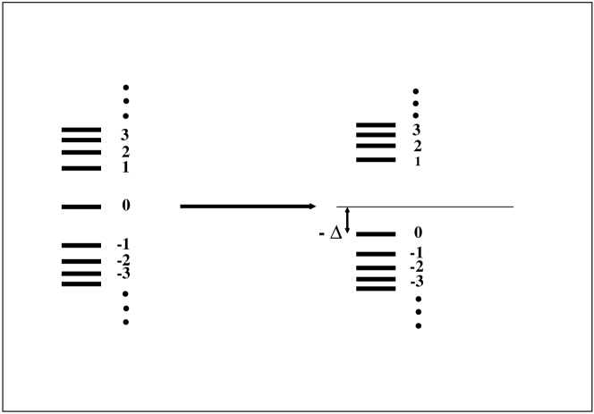
Figure 1: Schematic spectrum of Landau levels of surface states in topological insulators in applied magnetic field (left). Landau levels with dynamical generation of the gap $\Delta$ (right).

For convenience, in Fig. 1 we compare the spectrum of the Landau levels with $\Delta=0$ to the case of non-zero gap.
Thus, we can write:

$$\hat{\Psi}(\vec{x},t)=\int^{+\infty}_{-\infty}dp\;\left\{\sum^{\infty}_{n=1}e^{-i\frac{\varepsilon_{n}\;t}{\hslash}}\;\psi^{(+)}_{n,p}(\vec{x})\;\hat{b}_{n,p}\;+\;\sum^{\infty}_{n=0}e^{+i\frac{\varepsilon_{n}\;t}{\hslash}}\;\psi^{(-)}_{n,p}(\vec{x})\;\hat{d}^{\dagger}_{n,p}\;\right\}\;,$$ (4.14)

$$\hat{\Psi}^{\dagger}(\vec{x},t)=\int^{+\infty}_{-\infty}dp\;\left\{\sum^{\infty}_{n=1}e^{+i\frac{\varepsilon_{n}\;t}{\hslash}}\;\psi^{(+)\dagger}_{n,p}(\vec{x})\;\hat{b}^{\dagger}_{n,p}\;+\;\sum^{\infty}_{n=0}e^{-i\frac{\varepsilon_{n}\;t}{\hslash}}\;\psi^{(-)\dagger}_{n,p}(\vec{x})\;\hat{d}_{n,p}\;\right\}\;,$$ (4.15)

where the creation and annihilation operators operators satisfy the standard anticommutation relations, and

$$\varepsilon_{n}\;=\;\sqrt{2\hslash\frac{eB}{c}\,v_{F}^{2}\,n\,+\,\Delta_{0}^{2}}\;\;.$$ (4.16)

Whereupon, we obtain the Hamiltonian operator:

$$\hat{H}\;=\;\int^{+\infty}_{-\infty}dp\;\left\{\;\sum^{\infty}_{n=1}\varepsilon_{n}\;\hat{b}^{\dagger}_{n,p}\,\hat{b}_{n,p}\;+\;\sum^{\infty}_{n=0}\varepsilon_{n}\;\hat{d}^{\dagger}_{n,p}\,\hat{d}_{n,p}\right\}+E_{0}(B)\;,$$ (4.17)

with:

$$E_{0}(B)\;=\;-\;V\;\frac{eB}{2\pi\hslash c}\;\sum^{\infty}_{n=0}\,\varepsilon_{n}\;.$$ (4.18)

The renormalized Hamiltonian operator is:

$$\hat{H}_{R}\;=\;\int^{+\infty}_{-\infty}dp\;\left\{\;\sum^{\infty}_{n=1}\varepsilon_{n}\;\hat{b}^{\dagger}_{n,p}\,\hat{b}_{n,p}\;+\;\sum^{\infty}_{n=0}\varepsilon_{n}\;\hat{d}^{\dagger}_{n,p}\,\hat{d}_{n,p}\right\}+\Delta E_{0}(B)\;,$$ (4.19)

where now:

$$\Delta E_{0}(B)\;=\;-\;V\;\frac{eB}{2\pi\hslash c}\;\sum^{\infty}_{n=0}\,\sqrt{2\hslash\frac{eB}{c}\,v_{F}^{2}\,n\,+\,\Delta_{0}^{2}}\;-\;E_{0}\;.$$ (4.20)

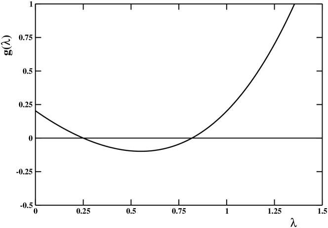
Figure 2: Plot of the function $g(\lambda)$, Eq. (4.27), versus $\lambda$.

To evaluate the (divergent) sum in Eq. (4.20) we employ the same trick as before. After some algebra it is easy to show that:

$$\sum^{\infty}_{n=0}\,\sqrt{2\hslash\frac{eB}{c}\,v_{F}^{2}\,n\,+\,\Delta_{0}^{2}}\;=\;+\,\Delta_{0}\;-\;\int_{0}^{\infty}\frac{ds}{\sqrt{\pi s}}\frac{d}{ds}\left[\frac{e^{-\Delta_{0}^{2}s}}{e^{+2\hslash v_{F}^{2}\frac{eB}{c}s}-1}\;\right]\;.$$ (4.21)

Since

$$\frac{e^{-\Delta_{0}^{2}s}}{e^{+2\hslash v_{F}^{2}\frac{eB}{c}s}-1}\;\stackrel{{\scriptstyle s\to 0}}{{\sim}}\;+\;\frac{1}{2\hslash v_{F}^{2}\frac{eB}{c}s}\;\;\;,$$ (4.22)

we readily obtain:

$$\Delta E_{0}(B)\;=\;V\;\frac{eB}{2\pi\hslash c}\;\left\{-\,\Delta_{0}\;+\;\int_{0}^{\infty}\frac{ds}{\sqrt{\pi s}}\frac{d}{ds}\left[\frac{e^{-\Delta_{0}^{2}s}}{e^{+2\hslash v_{F}^{2}\frac{eB}{c}s}-1}\;-\;\frac{1}{2\hslash v_{F}^{2}\frac{eB}{c}s}\;\right]\;\right\}\;.$$ (4.23)

Therefore the vacuum energy per particle is:

$$\varepsilon_{P}(B,\Delta_{0})\;=\;-\,\Delta_{0}\;+\;\int_{0}^{\infty}\frac{ds}{\sqrt{\pi s}}\frac{d}{ds}\left[\frac{e^{-\Delta_{0}^{2}s}}{e^{+2\hslash v_{F}^{2}\frac{eB}{c}s}-1}\;-\;\frac{1}{2\hslash v_{F}^{2}\frac{eB}{c}s}\;\right]\;\;.$$ (4.24)

Introducing the dimensionless variable:

$$\lambda\;=\;\frac{\Delta_{0}}{\sqrt{2\hslash v_{F}^{2}\frac{eB}{c}}}\;\;,$$ (4.25)

Eq. (4.24) can be rewritten as:

$$\varepsilon_{P}(B,\Delta_{0})\;=\;\sqrt{2\hslash v_{F}^{2}\frac{eB}{c}}\;\;g(\lambda)\;\;,$$ (4.26)

where:

$$g(\lambda)\;=\;-\,\lambda\;+\;\int_{0}^{\infty}\frac{dx}{\sqrt{\pi x}}\frac{d}{dx}\left[\frac{e^{-\lambda^{2}x}}{e^{x}-1}\;-\;\frac{1}{x}\;\right]\;\;.$$ (4.27)

It is straightforward to see that the function $g(\lambda)$ is finite. Indeed, in Fig. 2 we display $g(\lambda)$ versus $\lambda$. Eqs. (4.26) and (4.27) imply that the vacuum energy per particle depends not only on the magnetic field but also on the gap $\Delta_{0}$, which until now has been a free positive parameter. It is worthwhile to stress that for $\Delta_{0}=0$ Eq. (4.26) agrees with Eq. (3.15) since $g(0)\simeq 0.208$. Looking at Fig. 2 we note that the vacuum energy per particle decreases for small values of the gap $\Delta_{0}$, reaches a minimum, and then increases for large enough values of the gap. In fact, we find the minimum at $\lambda=\overline{\lambda}\simeq 0.56$ with $g(\overline{\lambda})\simeq-0.093$. To understand this peculiar behavior of the vacuum energy, we observe that the opening of the gap $\Delta_{0}$ affects the spectrum of the Landau levels in two way. On the one hand the gap decreases the energy of the zero modes (see Fig. 1). On the other hand the energy of higher Landau levels tend to increase with the gap. It is the balancing of these two effects that results in the vacuum energy minimum. Thus, we see that it is energetically favorable to induce a dynamical gap by a rearrangement of the Dirac sea triggered by quantum fluctuations. This remarkable phenomenon is quite analogous to the Peierls [26] quantum phase transition in quasi one-dimensional conductors.
In summary, we found that the low-lying surface states in three-dimensional topological insulators immersed in an external magnetic field give rise to gapped Landau levels:

$$\varepsilon_{n}^{(+)}\;=\;E_{D}(B)\;+\,\sqrt{2\hslash\frac{eB}{c}\,v_{F}^{2}\,n\,+\,\Delta_{0}^{2}}\;\;,\;\;n\,=\,1,\,2,\,...$$

$$\varepsilon_{n}^{(-)}\;=\;E_{D}(B)\;-\,\sqrt{2\hslash\frac{eB}{c}\,v_{F}^{2}\,n\,+\,\Delta_{0}^{2}}\;\;,\;\;n\,=\,0,\,1,\,...$$ (4.28)

with:

$$\Delta_{0}\;=\overline{\lambda}\;\sqrt{2\hslash v_{F}^{2}\frac{eB}{c}}\;\simeq\;0.56\;\sqrt{2\hslash v_{F}^{2}\frac{eB}{c}}\;,$$ (4.29)

and

$$E_{D}(B)\;\equiv\;E_{D}\;+\;\varepsilon_{P}(B,\Delta_{0})\;\simeq\;E_{D}\;-\,0.093\;\sqrt{2\hslash v_{F}^{2}\frac{eB}{c}}\;\;.$$ (4.30)

The results obtained in this Section rely on our effective Hamiltonian which should describe the low-lying excitations of the surface states in topological insulators. One must still face the task of comparing the results obtained within a highly-idealized model with experimental investigations of three-dimensional topological insulators.

5 Landau Levels: Comparison with Experimental Data

In the preceding Section we argued that it is energetically favored by quantum fluctuations to develop a mass gap for the low-lying surface excitations in three-dimensional topological insulator in an external magnetic field. The aim of this Section is to contrast our theoretical expectations to experimental data.
Quite recently, several experimental studies confirmed that the peculiar relativistic nature of surface states in topological insulators in magnetic fields leads to Landau levels which varies linearly with $\sqrt{nB}$. The authors of Ref. [27, 28] reported direct observation of Landau quantization of the topological surface states in Bi₂Se₃ in magnetic fields by using scanning tunneling microscopy and spectroscopy. Relativistic Landau levels are also observed in the tunneling spectra in a magnetic field [29] by using scanning tunneling spectroscopy on the surface of the topological insulator. Moreover, microwave spectroscopy has been applied to study cyclotron resonance due to intraband transitions between Landau levels in Bi₂Se₃ [30].
The hallmark of Dirac fermions for low-lying surface excitations in three-dimensional topological insulator is the presence of a field independent Landau level at the Dirac point (zero mode) and the already alluded scaling of higher Landau levels with $\sqrt{nB}$. In fact, Fig. 4 in Ref. [27] displays the energies of the Landau levels versus $\sqrt{nB}$ for magnetic fields ranging from 8 T to 11 T . Remarkably, for higher values of n one observes Landau level energies which vary linearly with $\sqrt{nB}$. Moreover, from Fig. 2 in Ref. [27] one infers that the lowest Landau level, assumed to be the zero mode $n=0$, is pinned at the Dirac point:

$$E_{D}\;\simeq\;-200\;mev\;\;,$$ (5.1)

consistently with the value inferred from the minimum of the differential tunneling conductance in absence of magnetic field. However, for low $n$, namely for the Landau levels with energies near the Dirac point, it seems that the Landau levels deviate from the linear behavior. We believe that this effect can be accounted for if we admit the presence of a dynamical mass gap according to our previous discussion in Sect. 4. To check quantitatively this, we need the energies of the Landau levels for different magnetic field strength. Fortunately, Fig. 2 in Ref. [28] reports the Landau levels for different magnetic fields ranging from 6 T up to 11 T. We used the experimental data extracted from Fig. 2 of Ref. [28] to perform a quantitative comparison with the theoretical results discussed in the previous Section. To this end, we note that in Refs. [27, 28] the energy of the Landau levels are determined by fitting the differential conductance with multiple gaussians. The typical peak width of Landau levels turns out to be of about 8 mev. Therefore, to be conservative, for our analysis we assumed for the Landau level energies a statistical uncertainty of about 2 - 3 mev.
Preliminarily, to check our procedure, we fitted the data to the expected spectrum of Landau levels for massless Dirac fermions, Eq. (1.1). Since the average Fermi velocity in Bi₂Se₃ lies in the range $v_{F}=3.0-7.0\times 10^{7}$ cm/s [31], we write $v_{F}=v_{5}\times 5.0\;10^{7}$ cm/s. Accordingly, for the spectrum lying above the Dirac point, Eq. (1.1) can be rewritten as:

$$\varepsilon^{(+)}_{n}\;=\;E_{D}\;+\;18.34\;mev\;v_{5}\;\sqrt{n\;B(T)}\;\;,\;\;n\;=\;0\,,\,1\,,\,2\,,\;.\,.\,,$$ (5.2)

where B(T) stands for magnetic field strength in Tesla.
To implement the fits we used the program Minuit [32] which is conceived as a tool to find the minimum value of a multi-parameter function and analyze the shape of the function around the minimum. The principal application is to compute the best-fit parameter values and uncertainties by minimizing the total chi-square $\chi^{2}$.

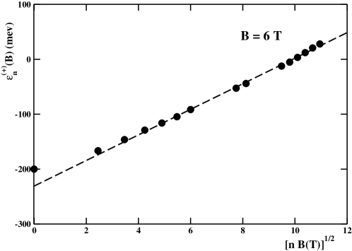
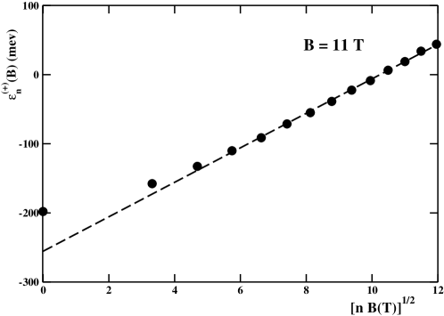
Figure 3: Landau level energies $\varepsilon_{n}^{(+)}(B)$ versus $\sqrt{nB}$ for B = 7 T (Top) and B = 11 T (Bottom). Data have been borrowed from Fig.2 of Ref. [28]. The assumed statistical errors are smaller than the symbol size. Dashed lines are the fits of $\varepsilon_{n}^{(+)}(B)$ to Eq. (5.2).

We fitted the experimental data to Eq. (5.2) for each values of the magnetic field leaving $E_{D}$ and $v_{5}$ as free fitting parameters. Moreover, to get a sensible fit to the data we excluded the Landau levels with $n=0,1$. In Table 1 we summarize the results of the fitting procedure. Note that in the last column of Table 1 we indicate the reduced chi-square, namely the total chi-square $\chi^{2}$ divided by the number of degree of freedom. As rule of thumb, a sensible fit results in $\chi_{r}^{2}\sim 1$.

Table 1: Summary of the values of fitting parameters in Eq. (5.2) reported, respectively, in the second and third columns. In the fourth column we give the reduced chi-square.

B(T)	$E_{D}$ (mev)	$v_{5}$	$\chi^{2}_{r}$
6	-231 $\pm$ 5	1.27 $\pm$ 0.03	1.20
7	-237 $\pm$ 5	1.29 $\pm$ 0.03	1.00
8	-249 $\pm$ 5	1.32 $\pm$ 0.03	1.05
9	-246 $\pm$ 5	1.30 $\pm$ 0.03	0.77
10	-251 $\pm$ 5	1.32 $\pm$ 0.03	0.95
11	-256 $\pm$ 6	1.36 $\pm$ 0.03	0.99

In Fig. 3 we display the experimental data together with the fitting lines for two representative values of the magnetic field. As it turns out, the lowest Landau level has an energy quite close to the Dirac point $E_{D}\simeq$ - 200 mev independently on the magnetic field strengths. However, the lowest Landau levels $n=0,1$ seems to deviate appreciably from the linear behavior $\sim\sqrt{nB}$ which fits nicely the $n\geq 2$ Landau levels. Even more, if we extrapolate $\varepsilon^{(+)}_{n}$ according to Eq. (5.2) we obtain the energies of the Dirac point, showed in Table 1, which, not only lie very far from the value at zero magnetic field, Eq. (5.1), but seem to decrease with the magnetic field. On the other hand, the fitted values of the Fermi velocity $v_{F}$ does not show a sizable dependence on the magnetic field strengths. In fact, in Fig. 4 we report the fitted values of the Fermi velocity versus the magnetic field strength. We find for the average Fermi velocity:

$$v_{F}\;=\;6.55\;\pm\;0.12\;10^{7}\;cm/s\;\;\;,\;\;\;\chi^{2}_{r}\;=\;1.07\;\;.$$ (5.3)

It is reassuring to see that $v_{F}$ in Eq. (5.3) lies in allowed range for the average Fermi velocity in Bi₂Se₃ [31].

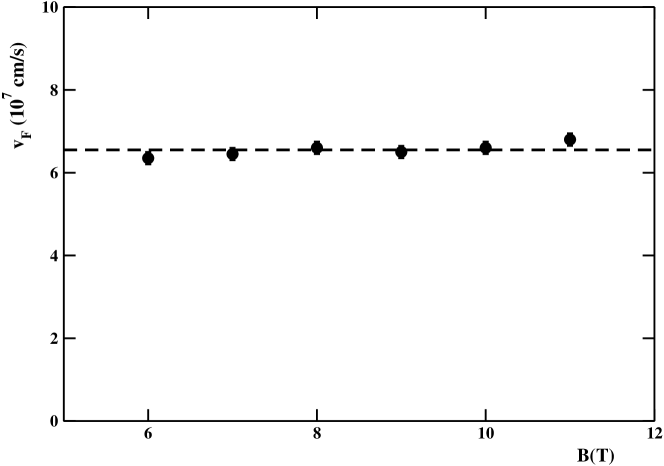
Figure 4: Fermi velocity in $10^{7}\;cm/s$ versus the magnetic field B(T). The dashed line is the average velocity, Eq.(5.3), obtained by fitting with a constant the values in Table 1.

The puzzling anomalies encountered within the standard interpretation of the measured Landau level energies point to an alternative interpretation of the experimental data. We shall, now, show that the measurements can be accounted for in a consistent manner within the theoretical scenario discussed in Sect. 4. In this case, the spectrum of the Landau levels is given by Eqs. (4), (4.29), and (4.30). To this end, we need the Landau levels which are above the Dirac point. According to Eq. (4) we have:

$$\varepsilon_{n}^{(+)}\;=\;E_{D}(B)\;+\,\sqrt{2\hslash\frac{eB}{c}\,v_{F}^{2}\,n\,+\,\Delta_{0}^{2}}\;\;,\;\;n\,=\,1,\,2,\,...\;,$$ (5.4)

with:

$$\Delta_{0}\;=\delta\;\sqrt{2\hslash v_{F}^{2}\frac{eB}{c}}\;\;,\;\;\delta\;\simeq\;0.56\;\;,$$ (5.5)

and

$$E_{D}(B)\;=\;E_{D}\;-\;\alpha\;\sqrt{2\hslash v_{F}^{2}\frac{eB}{c}}\;\;,\;\;\alpha\;\simeq\;0.093\;.$$ (5.6)

For convenience we rewrite Eq. (5.4) as:

$$\varepsilon^{(+)}_{n}\;=\;E_{D}(B)\;+\;18.34\;mev\;v_{5}\;\sqrt{B(T)\;(n\;+\;\delta^{2})}\;\;,\;\;n\;=\;1\,,\,2\,,\;.\,.\,.\;.$$ (5.7)

Table 2: Summary of the values of the fitting parameters in Eq. (5.7) reported, respectively, in the second, third and fourth columns. In the last column we give the reduced chi-square.

B(T)	$E_{D}(B)$ (mev)	$v_{5}$	$\delta$	$\chi^{2}_{r}$
6	-262.0 $\pm$ 4.2	1.39 $\pm$ 0.03	0.50 $\pm$ 0.36	1.33
7	-271.1 $\pm$ 4.4	1.42 $\pm$ 0.02	0.50 $\pm$ 0.36	1.21
8	-283.5 $\pm$ 4.4	1.44 $\pm$ 0.03	0.50 $\pm$ 0.42	0.92
9	-288.9 $\pm$ 4.5	1.45 $\pm$ 0.02	0.50 $\pm$ 0.35	0.67
10	-298.1 $\pm$ 4.6	1.48 $\pm$ 0.02	0.50 $\pm$ 0.35	0.76
11	-299.3 $\pm$ 4.9	1.49 $\pm$ 0.08	0.55 $\pm$ 0.13	0.42

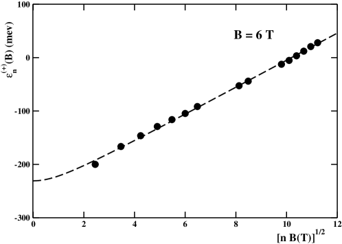
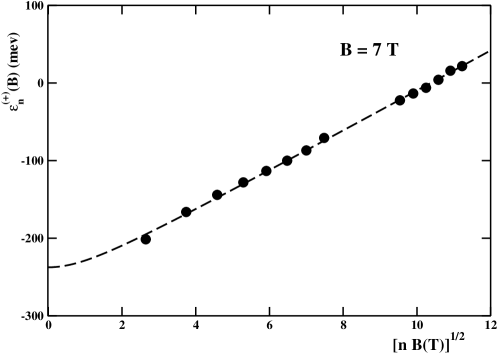
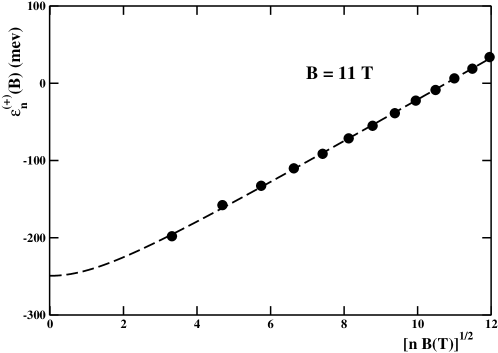
Figure 5: Landau level energies $\varepsilon^{(+)}_{n}$ versus $\sqrt{nB}$ for B = 6 T (Top), B = 7 T (Middle), and B = 11 T (Bottom). Data have been extracted form Fig.2 of Ref. [28]. The assumed statistical errors are smaller than the symbol size. Dashed lines are the fits of $\varepsilon_{n}^{(+)}(B)$ to Eq. (5.7).

We have fitted the available data to Eq. (5.7) leaving $E_{D}(B)$, $v_{5}$, and $\delta$ as free parameters. As a result, the fitting procedure gives the best fit values of the parameter for each given value of the magnetic field. For convenience, the results of our fits are summarize in Table 2, while in Fig. 5 we display the experimental data together with the fitting curves for three representative values of the magnetic field.
A few comments are in order. First, we note that the Dirac energy $E_{D}(B)$ do depend on the magnetic field as in the previous fits. However, presently we expect a shift of the Dirac point according to Eq. (5.6). In fact, as we will discuss later the shift of the Dirac point due to the magnetic field seems to be consistent with theoretical expectations. From Table 2 we see that the Fermi velocity is independent on the magnetic field strengths. In fact, we find for the average Fermi velocity:

$$v_{F}\;=\;7.2\;\pm\;0.1\;10^{7}\;cm/s\;\;\;,\;\;\;\chi^{2}_{r}\;=\;1.67\;\;.$$ (5.8)

This value of the Fermi velocity is slightly higher, but in reasonable agreement with our previous determination Eq. (5.3).
As concern the spectrum of the Landau levels, we stress that the levels lying above the Dirac point have $n\geq 1$, according to Eq. (5.7). In fact, the zero mode $n=0$ has been pushed below $E_{D}(B)$ due to the dynamical generation of the mass gap. Therefore, Fig. 5 shows that our theoretical curves are able to track all the experimental data. Note that the lowest Landau level $n=1$ has an energy which seems to be almost independent on the magnetic field. This is due to the compensation of two different effects. Indeed, the increase of the energy due to the magnetic field for $n\neq 0$ is contrasted by the negative shift of the Dirac point. For $n=1$ these two effects almost perfectly compensate each other. From Fig. 5 and Table 2 we may conclude that the data are in reasonable agreement with Eq. (5.7) for all the available values of the magnetic field. Note that in Fig. 5, to magnify the non linearity in $\sqrt{nB}$ due to the gap, the fitting curves have been draw starting from $nB=0$. Concerning the parameter $\delta$, looking at Table 2 we see that this parameter does not depend on the magnetic field. We find for the average value:

$$\delta\;=\;0.51\;\pm\;0.18\;\;\;,\;\;\;\chi^{2}_{r}\;=\;0.01\;\;,$$ (5.9)

which is in remarkable agreement with our theoretical expectations.

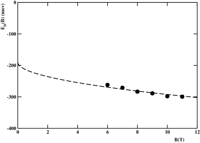
Figure 6: Dirac point energies $E_{D}$ in meV versus the magnetic field B in Tesla. Dashed line is the fit of $E_{D}(B)$ to Eq.(5.6).

Finally, we must check if the dependence of the Dirac energy on the magnetic field is in agreement with Eq. (5.6). In Fig. 6 we report the fitted values of the Dirac energy in Table 2 as a function of the magnetic field. We have fitted these values according to Eq. (5.6) assuming for the Fermi velocity the average value Eq. (5.8), and leaving $E_{D}$ and $\alpha$ as free parameters. The fit returns for these two parameters the following values:

$$E_{D}\;=\;-\;190\;\pm\;14\;mev\;\;,\;\;\;\alpha\;=\;1.22\;\pm\;0.04\;\;,\;\;\;\chi^{2}_{r}\;=\;1.53\;\;.$$ (5.10)

Indeed, we find that the shift of the Dirac point with the magnetic field is in satisfying agreement with Eq. (5.6) (see dashed line in Fig. 6). Moreover, the parameter $E_{D}$, which is the energy of the Dirac point in absence of the magnetic field, is in good agreement with the experimental value Eq. (5.1). However, we must stress that the parameter $\alpha$ is well above our theoretical estimate, Eq. (5.6). We recall that this parameter quantify the vacuum energy per particle. In our opinion, since the calculations in previous Section have been performed within a highly idealized model, such a discrepancy does not spoil the overall coherent agreement of our theoretical picture with the experimental observations.

6 Quantum Hall Effect and Chiral Edge States

The Hall effect indicates the voltage drop across a conductor transverse to the direction of the applied electrical current in the presence of a perpendicular magnetic field. In the quantum Hall effect, with increasing magnetic field, the Hall resistance evolves from a straight line into step-like behaviors with well-defined plateaux. At the plateaux the Hall conductance is quantized :

$$\sigma_{xy}\;=\;\frac{e^{2}}{2\pi\hslash}\;\nu\;\;,\;\;$$ (6.1)

where $\nu$ is an integer or a certain fraction. At the same time, the longitudinal resistance drops to zero, suggesting dissipationless transport of charged quasiparticles.
A single two-dimensional Dirac fermion under a magnetic field is known to show the quantized Hall effect with the Hall conductance:

$$\sigma_{xy}\;=\;\frac{e^{2}}{2\pi\hslash}\;(n\;+\;\frac{1}{2})\;,$$ (6.2)

$n$ being an integer. The factor $1/2$ in Eq. (6.2) is characteristic of the relativistic dispersion relation of Dirac fermions compared with the usual massive electrons, and it is related to the zero modes pinned at the neutral point. Alternatively, the half-integer quantization can be also accounted for as a Berry phase [33, 34]. The Hall conductance of three dimensional topological insulators is expected to be given by the sum of the contributions from the top and bottom surfaces (see Fig. 7, left panel). Therefore one finds:

$$\sigma_{xy}\;=\;\frac{e^{2}}{2\pi\hslash}\;(n\;+\;m\;+\;1)\;,$$ (6.3)

with $n$ and $m$ are integers referring to the upper and lower surface respectively.

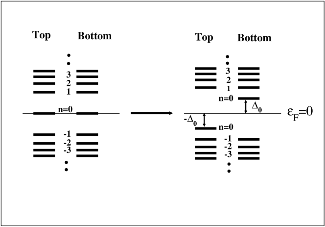
Figure 7: Schematic spectrum of surface state Landau levels in applied magnetic field (left). Landau levels with dynamical generation of a gap $\Delta_{0}$ (right). The Fermi level is at Dirac neutral point $\varepsilon_{F}=0$.

When the Landau levels of the top and bottom surface coincide exactly, the two contributions are equivalent and one has $n=m$, namely only the odd integer quantum Hall effect is expected. If, however, the degeneracy of the Landau levels is removed, then the Hall conductance becomes quantized as integers. Indeed, recently the integer quantum Hall effect has been observed in three dimensional topological insulators [35, 36].
If we admit the generation of a dynamical mass gap, then, according to Eq. (4.5) we obtain the gapped Landau level spectrum for the two surfaces as displayed in Fig. 7, right panel. In fact, we adopted the convention that magnetic fields perpendicular to the surfaces are positive in the direction of the outward surface normal, so that the transverse magnetic field is positive for the top surface and negative for the bottom surface. It is evident that also in this case we obtain the odd integer quantum Hall effect for identical surfaces, or the integer quantum Hall effect if the the degeneracy of the Landau levels in the top and bottom surfaces is removed.
Interestingly enough, in high magnetic fields an additional quantum Hall plateau at the charge neutral point with $\nu$ = 0 has been observed [36]. This peculiar zero-Hall plateau could be explained in a natural way if there are gapless edge excitations pinned at the Dirac neutral point. Indeed, it has been already proposed [37] that chiral edge states residing at the magnetic domain boundaries are responsible for the zero-Hall plateau observed in the quantum anomalous Hall effect in magnetic topological insulators. More recently, chiral edge states residing at the magnetic domain boundaries on the surface of a three-dimensional topological insulator have been observed by means of a scanning superconducting quantum interference device [38].
In this Section we discuss the presence of current-carrying chiral edge states residing at the magnetic domain boundaries between the top and bottom surfaces of a three-dimensional insulator. Moreover, these peculiar edge excitations are pinned at the Dirac neutral point, whereas the energy spectrum of the surface states is gapped. It turns out that these states are localized on the magnetic domain wall and are similar to the Jackiw-Rebbi soliton [39].
To face this task, in Fig. 8 we show a schematic picture of the magnetic field on the upper and lower surfaces of a three-dimensional topological insulator. At the edges of the surfaces the magnetic field decreases to zero within a region of linear size given by the magnetic length:

$$a_{B}\;=\;\sqrt{\frac{\hslash c}{eB_{0}}}\;.$$ (6.4)

The physical meaning of Eq. (6.4) is as follows. The low-lying quantum states localized on the upper surface will feel a magnetic field which is positive and vanishes near the surface boundaries within a distance of order $\sim a_{B}$. Obviously, the same happens on the lower surface where the magnetic field is negative. If we glue together the two surfaces along an edge, as shown in Fig.  8, we see that the surface excitations will be subject to an effective magnetic field which can be written as:

$$B(x)\;=\;B_{0}\;tgh\left[\sqrt{\frac{eB_{0}}{\hslash c}}\;x\right]\;,$$ (6.5)

where $B_{0}$ is the strength of the (constant) magnetic field inside the two surfaces. Accordingly, the potential vector is given by:

$$\vec{A}(x,y)\;=\;\left(-B(x)\;y\;\;,\;\;0\right)\;\;.$$ (6.6)

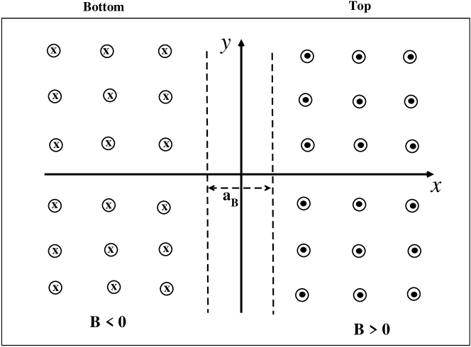
Figure 8: Schematic picture of the magnetic kink relevant for the edge states. Dots and crosses indicate the direction of magnetic field leaving and entering the surface, respectively. The width of the strip (dashed lines) where the magnetic field change sign is set by the magnetic length $a_{B}=\sqrt{\frac{\hslash c}{eB_{0}}}$.

Let us consider, now, the Dirac equation in presence of the magnetic field given by Eq. (6.5). After taking into account Eq. (6.6), we readily obtain:

$$\left(\begin{array}[]{cc}0&\hslash\partial_{x}-i\frac{e}{c}B(x)y-i\hslash\partial_{y}\\ -\hslash\partial_{x}+i\frac{e}{c}B(x)y-i\hslash\partial_{y}&0\end{array}\right)\psi(x,y)\;=\;\frac{\varepsilon}{v_{F}}\psi(x,y)\;,$$ (6.7)

Note that in Eq. (6.7) we do not consider the mass gap $\Delta_{0}$. In fact, we are interested here in the zero-energy solutions that are localized at the surface boundary $x=0$ where the magnetic field vanishes. Let $\Theta(x,y)$ be the solutions of Eq. (6.7) with $\varepsilon=0$. Writing:

$$\Theta(x,y)\;=\;\left(\begin{array}[]{c}\theta_{1}(x,y)\\ \theta_{2}(x,y)\end{array}\right)\;,$$ (6.8)

we get:

$$\begin{array}[]{c}\left[+\hslash\partial_{x}-i\frac{e}{c}B(x)y-i\hslash\partial_{y}\right]\theta_{2}(x,y)\;=\;0\\ \;\;\;\left[-\hslash\partial_{x}+i\frac{e}{c}B(x)y-i\hslash\partial_{y}\right]\theta_{1}(x,y)\;=\;0\;\;.\end{array}$$ (6.9)

Let us consider, firstly, the region $x>0$. For $x\gg a_{B}$ evidently $B(x)\simeq B_{0}$. In this case we have already seen that the solution of Eq. (6.9) is given by Eq. (3.14). This suggests to seek the solutions of Eq. (6.9) in the form:

$$\Theta_{+}(x,y)\;=\;\left(\begin{array}[]{c}0\\ \theta(x,y)\end{array}\right)\;\;,\;\;x\;>\;0\;\;.$$ (6.10)

Inserting Eq. (6.10) into Eq. (6.9) we obtain the equation for $\theta(x,y)$ which we rewrite as:

$$\left\{+\hslash\partial_{x}-i\frac{e}{c}[B(x)-B_{0}]y-i\frac{e}{c}B_{0}y-i\hslash\partial_{y}\right\}\theta(x,y)\;=\;0\;\;.$$ (6.11)

To solve this last equation, we write:

$$\theta(x,y)\;=\;e^{-i\frac{e}{\hslash c}y\int^{+\infty}_{x}[B(x^{\prime})-B_{0}]dx^{\prime}}\;\;\tilde{\theta}(x,y)\;\;,$$ (6.12)

to get:

$$\left\{+\hslash\partial_{x}-i\frac{e}{c}B_{0}y-\frac{e}{c}\int^{+\infty}_{x}[B(x^{\prime})-B_{0}]dx^{\prime}-i\hslash\partial_{y}\right\}\;\tilde{\theta}(x,y)\;=\;0\;\;.$$ (6.13)

To proceed further, we put:

$$\tilde{\theta}(x,y)\;=\;\tilde{\theta}_{p}(x,y)\;=\;f(x)\;e^{ipx}\;\Phi_{0,p}(y)\;\;,$$ (6.14)

where:

$$\Phi_{0,p}(y)\;=\;e^{-\frac{1}{2}{\zeta}^{2}}\;,\;\zeta\,=\,\sqrt{\frac{eB_{0}}{\hslash c}}\left(y-\frac{cp}{eB_{0}}\right)\;\;.$$ (6.15)

After some manipulations, we finally get:

$$\frac{f^{\prime}(x)}{f(x)}\;=\;\sqrt{\frac{eB_{0}}{\hslash c}}\;g(x\sqrt{\frac{eB_{0}}{\hslash c}})\;\;,\;\;g(z)\;=\;-\,ln\left[1\;+\;e^{-2\,z}\right]\;\;,$$ (6.16)

giving:

$$f(x)\;=\;{\cal{N}}\;e^{\sqrt{\frac{eB_{0}}{\hslash c}}\;\int^{x}_{0}g(x^{\prime}\sqrt{\frac{eB_{0}}{\hslash c}})dx^{\prime}}\;\;.$$ (6.17)

To a good approximation, for $x\lesssim a_{B}$, we can rewrite Eq. (6.17) as:

$$f(x)\;\simeq\;{\cal{N}}\;e^{-\;ln2\;\sqrt{\frac{eB_{0}}{\hslash c}}\;x}\;\;.$$ (6.18)

Putting it all together, we end with:

$$\Theta_{+}(x,y)\;=\;\left(\begin{array}[]{c}0\\ \theta_{p}(x,y)\end{array}\right)\;\;,\;\;x\;>\;0\;\;,$$ (6.19)

where:

$$\theta_{p}(x,y)\;=\;e^{-i\frac{e}{\hslash c}y\int^{+\infty}_{x}[B(x^{\prime})-B_{0}]dx^{\prime}}\;\;\tilde{\theta}_{p}(x,y)\;\;,$$ (6.20)

and

$$\tilde{\theta}_{p}(x,y)\;=\;{\cal{N}}\;e^{-\;ln2\;\sqrt{\frac{eB_{0}}{\hslash c}}\;|x|}\;e^{ipx}\;\Phi_{0,p}(y)\;\;.$$ (6.21)

It is easy to check that for $x<0$ the solutions of Eq. (6.9) are given by :

$$\Theta_{-}(x,y)\;=\;\left(\begin{array}[]{c}\theta_{-p}(x,y)\\ 0\end{array}\right)\;\;,\;\;x\;<\;0\;\;.$$ (6.22)

It is worthwhile to stress that the two zero-energy modes $\Theta_{\pm}(x,y)$ are localized in the region $|x|\lesssim\sqrt{\frac{\hslash c}{eB_{0}}}$, and are related by parity and time-reversal transformations. Therefore, if the chemical potential is tuned to the Dirac neutral point, then the zero-energy edge modes will contribute to the conductivity. In particular, it is evident that the contributions of these modes cancel exactly in the Hall conductance $\sigma_{xy}=0$, while they add to the longitudinal conductance $\sigma_{xx}=\sigma_{yy}>0$. So that, we see that these edge modes give rise to the Hall plateau at the charge neutral point with $\nu$ = 0, but with a finite longitudinal resistance at variance of the usual Hall plateaux where the longitudinal resistance vanishes.

7 Summary and Conclusions

In this work, we have discussed the dynamics of low-lying surface excitation in three-dimensional topological insulators. We developed a quantum field theoretical description for the surface states of three-dimensional topological insulators, which allowed us to investigate the quantum dynamics of low-lying surface states in presence of an applied transverse magnetic field.
We evaluated the effects of quantum fluctuations on the ground state. In particular, we argued that, in presence of a constant transverse magnetic field, the quantum fluctuations induce a shift of the energy of the Dirac neutral point which, in turns, depends on the strength of the magnetic field. Moreover, we argued that low-lying surface excitations in three-dimensional topological insulators develop a mass gap varying with $\sqrt{eB}$ by a rearrangement of the Dirac sea induced by quantum fluctuations. Interestingly enough, very recently the physical consequences of dynamical mass generation in several classes of topological Dirac metals have been discussed in Ref. [40].
To compare our theoretical scenario with observations, we reanalyzed the available experimental data for the Landau level spectrum of the surface states in three-dimensional topological insulators. Remarkably, we argued that our theoretical results allowed a consistent and coherent description of the Landau level spectrum of the surface low-lying excitations.
Finally, we showed that recently detected zero-Hall plateau at the charge neutral point could be accounted for by chiral edge states residing at the magnetic domain boundaries between the top and bottom surfaces of three-dimensional topological insulators.

Appendix A Appendix

We collect here some intermediate steps needed in the derivation of results presented in Sects. 2 and 3. Firstly, let us consider the positive and negative energy solutions of the following Dirac equation:

$$-i\,\hslash\,v_{F}\;\vec{\alpha}\cdot\vec{\nabla}\;\psi^{(\pm)}(\vec{x})\;=\;\pm\;\varepsilon_{\vec{p}}\;\psi^{(\pm)}(\vec{x})\;,$$ (A.1)

It is quite easy to solve Eq. (A.1):

$$\psi^{(+)}_{\vec{p}}(\vec{x})\;=\;\frac{1}{2\pi\hslash}\;e^{+i\,\frac{\vec{p}\cdot\vec{x}}{\hslash}}\;u_{\vec{p}}\;\;,\;\;\psi^{(-)}_{\vec{p}}(\vec{x})\;=\;\frac{1}{2\pi\hslash}\;e^{-i\,\frac{\vec{p}\cdot\vec{x}}{\hslash}}\;v_{\vec{p}}\;\;,\;\;\varepsilon_{\vec{p}}\;=\;v_{F}\;|\vec{p}|\;,$$ (A.2)

where:

$$u_{\vec{p}}\;=\;\frac{1}{\sqrt{2}}\left(\begin{array}[]{c}1\\ -i\;e^{+i\theta_{\vec{p}}}\end{array}\right)\;\;,\;\;v_{\vec{p}}\;=\;\frac{1}{\sqrt{2}}\left(\begin{array}[]{c}1\\ +i\;e^{+i\theta_{\vec{p}}}\end{array}\right)\;\;,\;\;\tan\theta_{\vec{p}}\;=\;\frac{p_{y}}{p_{x}}\;.$$ (A.3)

Note that the positive and negative energy solutions of the Dirac equation are normalized according to:

$$\int d^{2}x\;[\psi^{(\pm)}_{\vec{p^{\prime}}}(\vec{x})]^{\dagger}\;\psi^{(\pm)}_{\vec{p}}(\vec{x})\;=\;\delta(\vec{p}-\vec{p^{\prime}})\;.$$ (A.4)

Moreover, the Pauli spinors $u_{\vec{p}}$ and $v_{\vec{p}}$ satisfy the following relations:

$$u_{\vec{p}}\;u^{\dagger}_{\vec{p}}\;+\;v_{\vec{p}}\;v^{\dagger}_{\vec{p}}\;=\;\mathbb{I}\;=\left(\begin{array}[]{cl}1&0\\ 0&1\end{array}\right)\;\;,\;\;u^{\dagger}_{\vec{p}}\;v_{-\vec{p}}\;=\;0\;.$$ (A.5)

With the aid of Eqs. (A.4) and (A.5) one can verify that the anticommutation relations Eq. (2.9) are indeed equivalent to the canonical equal time anticommutation relations Eq. (2.6).
Next, we are interested in the Dirac equation in presence of an external magnetic field:

$$v_{F}\;\vec{\alpha}\cdot\left[-i\hslash\vec{\nabla}\;+\;\frac{e}{c}\vec{A}(\vec{x})\right]\psi(\vec{x})\;=\;\varepsilon\;\psi(\vec{x})\;.$$ (A.6)

Since we are interested in uniform magnetic fields perpendicular to the crystal surfaces, in the Landau gauge we can write:

$$A_{k}(x_{1},x_{2})\;=\;-x_{2}\;B\;{\delta}_{k,1}\;\;\;\;k=1,2\;.$$ (A.7)

As it is well known, in this case the Dirac equation Eq. (A.6) can be exactly solved (see, for instance, Ref. [20]). Indeed, Eq. (A.6) leads to:

$$\left(\begin{array}[]{cc}0&\hslash\partial_{1}-i\frac{eB}{c}x_{2}-i\hslash\partial_{2}\\ -\hslash\partial_{1}+i\frac{eB}{c}x_{2}-i\hslash\partial_{2}&0\end{array}\right)\psi(\vec{x})\;=\;\frac{\varepsilon}{v_{F}}\psi(\vec{x})\;,$$ (A.8)

with $\partial_{i}=\frac{\partial}{\partial x_{i}},i=1,2$. Writing:

$$\psi(\vec{x})\;=\;e^{i\frac{px_{1}}{\hslash}}\left(\begin{array}[]{c}\phi_{1}(x_{2})\\ \phi_{2}(x_{2})\end{array}\right)\;,$$ (A.9)

we obtain:

$$\begin{array}[]{c}\left[ip-i\frac{eB}{c}x_{2}-i\hslash\partial_{2}\right]\phi_{2}(x_{2})\;=\;\frac{\varepsilon}{v_{F}}\phi_{1}(x_{2})\\ \left[-ip+i\frac{eB}{c}x_{2}-i\hslash\partial_{2}\right]\phi_{1}(x_{2})\;=\;\frac{\varepsilon}{v_{F}}\phi_{2}(x_{2})\;.\end{array}$$ (A.10)

Inserting the second equation into the first we rewrite Eq. (A.10) as:

$$\begin{array}[]{c}\left[-\frac{\hslash^{2}}{2}\partial_{2}^{2}+\frac{1}{2}\frac{e^{2}B^{2}}{c^{2}}(x_{2}-\frac{pc}{eB})^{2}\right]\phi_{1}(x_{2})\;=\;\frac{1}{2}\left[(\frac{\varepsilon}{v_{F}})^{2}-\frac{\hslash eB}{c}\right]\phi_{1}(x_{2})\\ \phi_{2}(x_{2})\;=\;\frac{v_{F}}{\varepsilon}\left[-ip+i\frac{eB}{c}x_{2}-i\hslash\partial_{2}\right]\phi_{1}(x_{2})\;.\end{array}$$ (A.11)

The first equation in Eq. (A.11) is the familiar harmonic oscillator equation. Thus, we can write:

$$\phi_{1}(x_{2})\;=\;\Phi_{n,p}(x_{2})\;\;,\;\;\Phi_{n,p}(x_{2})\;=\;N_{n}\;H_{n}(\zeta)\;e^{-\frac{1}{2}{\zeta}^{2}}\;,$$ (A.12)

where:

$$N_{n}=\left(\frac{eB}{\pi\hslash c}\right)^{\frac{1}{4}}\frac{1}{\sqrt{2^{n}n!}}\;\;,\;\;\zeta\,=\,\sqrt{\frac{eB}{\hslash c}}\left(x_{2}-\frac{cp}{eB}\right)\;,$$ (A.13)

and $H_{n}(x)$ being the Hermite’s polynomial of order $n$. Note that our normalization is such that:

$$\int^{+\infty}_{-\infty}dx_{2}\;\left|\Phi_{n,p}(x_{2})\right|^{2}\;=1\;.$$ (A.14)

Moreover, the energy eingenvalues are:

$$\varepsilon\;=\;\pm\,v_{F}\,\sqrt{2\hslash\frac{eB}{c}(n\,+\,1)}\;\;,\;\;n\,=\,0,\,1,\,...$$ (A.15)

One, also, easily find that:

$$\phi_{2}(x_{2})\;=\;\pm\;\Phi_{n+1,p}(x_{2})\;.$$ (A.16)

Therefore, we are lead to the following eigenfunctions:

$$\psi^{(\pm)}_{n,p}(x_{1},x_{2})\;=\;\frac{e^{\pm ipx_{1}}}{\sqrt{2\pi\hslash}}\;\frac{1}{\sqrt{2}}\left(\begin{array}[]{c}\Phi_{n,\pm p}(x_{2})\\ \pm\,i\,\Phi_{n+1,\pm p}(x_{2})\end{array}\right)$$ (A.17)

with energy eigenvalues given by Eq. (A.15), respectively. It is easy to see that there also zero mode solutions:

$$\psi_{0,p}(x_{1},x_{2})\;=\;\frac{e^{ipx_{1}}}{\sqrt{2\pi\hslash}}\;\left(\begin{array}[]{c}0\\ \Phi_{0,p}(x_{2})\end{array}\right)\;,$$ (A.18)

with energy eigenvalue:

$$\varepsilon_{0}\;=\;0\;\;.$$ (A.19)

If we adopt the convention that:

$$\Phi_{n,p}(x_{2})\;=\;0\;\;\;\text{if}\;\;\;n\;<\;0\;,$$ (A.20)

then we can write:

$$\psi^{(\pm)}_{n,p}(x_{1},x_{2})\;=\;\frac{e^{\pm ipx_{1}}}{\sqrt{2\pi\hslash}}\;\frac{1}{\sqrt{2}}\left(\begin{array}[]{c}\Phi_{n-1,\pm p}(x_{2})\\ \pm\,i\,\Phi_{n,\pm p}(x_{2})\end{array}\right)\;\;\;n\;=\;1,\;2,\;....$$ (A.23)

$$\psi_{0,p}(x_{1},x_{2})\;=\;\frac{e^{+ipx_{1}}}{\sqrt{2\pi\hslash}}\;\left(\begin{array}[]{c}0\\ \Phi_{0,p}(x_{2})\end{array}\right)\;\;\;n\;=\;0\;.$$ (A.26)

with energy eigenvalues:

$$\varepsilon_{0}\;=\;0\;\;,\;\;\varepsilon_{n}^{(\pm)}\;=\;\pm\;\varepsilon_{n}\;=\;\pm\,v_{F}\,\sqrt{2\hslash\frac{eB}{c}\,n}\;\;,\;\;n\,=\,1,\,2,\,...$$ (A.27)

The wave functions in Eq. (A.23) are normalized as:

$$\int^{+\infty}_{-\infty}d^{2}x\;{\psi^{(\pm)}_{n,p}}^{{\dagger}}(\vec{x})\;\psi^{(\pm)}_{n^{\prime},p^{\prime}}(\vec{x})\;=\;\delta(p-p^{\prime})\;\delta_{n,n^{\prime}}\;.$$ (A.28)

Note that the Landau levels are infinitely degenerate with density of states:

$$\int^{+\infty}_{-\infty}dp\;{\psi^{(\pm)}_{n,p}}^{{\dagger}}(\vec{x})\;\psi^{(\pm)}_{n,p}(\vec{x})=\frac{eB}{2\pi\hslash c}\;.$$ (A.29)

To derive Eq. (3.11) we note that by using Eq. (2.20) we may write:

$$E_{0}(B)=-\frac{eB}{2\pi\hslash c}V\sum_{n=0}^{\infty}\varepsilon_{n}\,=\frac{eB}{2\pi\hslash c}\,V\sum_{n=0}^{\infty}\int_{0}^{\infty}\frac{ds}{\sqrt{\pi s}}\frac{d}{ds}\left(e^{-2\hslash v_{F}^{2}\frac{eB}{c}\,n\,s}\right)\;.$$ (A.30)

We may, now, perform the summation over $n$:

$$\sum_{n=0}^{\infty}e^{-2\hslash v_{F}^{2}\frac{eB}{c}\,n\,s}\;=\;\frac{1}{1-e^{-2\hslash v_{F}^{2}\frac{eB}{c}\,s}}\;,$$ (A.31)

to obtain:

$$E_{0}(B)\;=\;\frac{eB}{2\pi\hslash c}\,V\int_{0}^{\infty}\frac{ds}{\sqrt{\pi s}}\frac{d}{ds}\left(\frac{1}{1-e^{-2\hslash v_{F}^{2}\frac{eB}{c}s}}\right)\;.$$ (A.32)

As discussed in Sect. 2, the ultraviolet divergences in $E_{0}(B)$ are recovered from the singularity for $s\to 0$. To isolate the divergent part in Eq. (A.32), we note that:

$$\frac{1}{1-e^{-2\hslash v_{F}^{2}\frac{eB}{c}s}}\;\stackrel{{\scriptstyle s\to 0}}{{\sim}}\;+\;\frac{1}{2\hslash v_{F}^{2}\frac{eB}{c}s}\;\;\;.$$ (A.33)

This suggests to rewrite Eq. (A.32) as:

$$E_{0}(B)\;= \;\frac{eB}{2\pi\hslash c}\,V\int_{0}^{\infty}\frac{ds}{\sqrt{\pi s}}\frac{d}{ds}\left[\frac{1}{1-e^{-2\hslash v_{F}^{2}\frac{eB}{c}s}}\;-\;\frac{1}{2\hslash v_{F}^{2}\frac{eB}{c}s}\right]\;$$ (A.34)

$$+\;\frac{eB}{2\pi\hslash c}\,V\int_{0}^{\infty}\frac{ds}{\sqrt{\pi s}}\frac{d}{ds}\frac{1}{2\hslash v_{F}^{2}\frac{eB}{c}s}\;.$$

The divergent term in $E_{0}(B)$ is due to the second integral in the right-hand part of Eq. (A.34). Comparing with Eq. (2.21) we at once recognize that this divergent term coincides with $E_{0}$. Therefore, we obtain:

$$\Delta E_{0}(B)\;=\;E_{0}(B)\,-\,E_{0}\;=\frac{eB}{2\pi\hslash c}\,V\int_{0}^{\infty}\frac{ds}{\sqrt{\pi s}}\frac{d}{ds}\left[\frac{1}{1-e^{-2\hslash v_{F}^{2}\frac{eB}{c}s}}\;-\;\frac{1}{2\hslash v_{F}^{2}\frac{eB}{c}s}\right]\;,$$ (A.35)

which agrees with Eq. (3.11).

References

- [1] M. Z. Hasan and C. L. Kane, Rev. Mod. Phys. 82 (2010) 3045
- [2] J. E. Moore, Nature 464 (2010) 194
- [3] M. Z. Hasan and J. E. Moore, Ann. Rev. Cond. Mat. Phys. 2 (2011) 55
- [4] X.- L. Qi and S.-C. Zhang, Rev. Mod. Phys. 83 (2011) 1057
- [5] M. Fruchart and D. Carpentier, Comp. Rend. Phys. 14 (2013) 779
- [6] Y. Ando, J. Phys. Soc. Jpn. 82 (2013) 102001
- [7] O. Vafek and A. Vishwanath, Ann. Rev. Cond. Mat. Phys. 5 (2014) 83
- [8] T. O. Wehling, A. M. Black-Schaffer, and A. V. Balatsky, Adv. Phys. 76 (2014) 1
- [9] M. Zahid Hasan, S.-Y. Xu, D. Hsieh, L. A. Wray, Y. Xia, Experimental Discovery of Topological Surface States - A New Type of 2D Electron Systems (2014) arXiv:1401.0848
- [10] M. Zahid Hasan, S.-Y. Xu, M. Neupane, Topological Insulators, Topological Crystalline Insulators, Topological Semimetals and Topological Kondo Insulators (2014) arXiv:1406.1040
- [11] L. Fu, C. L. Kane, and E. J. Mele, Phys. Rev. Lett. 98 (2007) 106803
- [12] A. K. Geim and K. S. Novoselov, Nature Materials 6 (2007) 183
- [13] M. I. Katsnelson, Materials Today 10 (2007) 20
- [14] A. H. Castro Neto, F. Guinea, N. M. R. Peres, K. S. Novoselov, and A. K. Geim, Rev. Mod. Phys. 81 (2009) 109
- [15] V. N. Kotov, B. Uchoa, V. M. Pereira, A. H. Castro Neto, and F. Guinea, Rev. Mod. Phys. 84 (2012) 1067
- [16] H. B. Nielsen and M. Ninomiya, Phys. Lett. B 130 (1983) 389
- [17] J.D. Bjorken and S.D. Drell, Relativistic Quantum Fields, McGraw-Hill Book Company, New York (1968)
- [18] P. Cea, Phys. Rev. D 32 (1985) 2785; Phys. Rev D 34 (1986) 3229
- [19] S. S. Schweber, An Introduction to Relativistic Quantum Field Theory, Row, Peterson and Company, Evanston, Illinois (1961)
- [20] A.I. Akheizer and V.B. Berestetsky, Quantum Electrodynamics, Interscience, New York (1965)
- [21] P. Cea, Mod. Phys. Lett. B 26 (2012) 1250084
- [22] B. S. Kandemir and A. Mogulkoc, Phys. Lett. A 379 (2015) 2120
- [23] R.Jackiw and S. Templeton, Phys. Rev. D 23 (1981) 2291
- [24] J. Schonfeld, Nucl. Phys. B 185 (1981) 157
- [25] S. Deser, R. Jackiw, and S. Templeton, Ann. Phys. 140 (1982) 372
- [26] R. E. Peierls, Quantum Theory of Solids, Oxford University Press, New York, London (1955)
- [27] P. Cheng, et al., Phys. Rev. Lett. 105 (2010) 076801
- [28] P. Cheng, et al., Landau Quantization of Massless Dirac Fermions in Topological Insulator (2010) arXiv:1001.3220
- [29] T. Hanaguri, K. Igarashi, M. Kawamura, H. Takagi, and T. Sasagawa, Phys. Rev. B 82 (2010) 081305
- [30] A. Wolos, S. Szyszko, A. Drabinska, M. Kaminska, S. G. Strzelecka, A. Hruban, A. Materna, and M. Piersa, Phys. Rev. Lett. 109 (2012) 247604
- [31] D. Kim, S. Cho, N. P. Butch, P. Syers, K. Kirshenbaum, S. Adam, J. Paglione, and M. S. Fuhrer, Nat. Phys. 8 (2012) 459
- [32] F. James and M. Roos, Comput. Phys. Comm. 10 (1975) 343
- [33] K. S. Novoselov, A. K. Geim, S. V. Morozov, D. Jiang, M. I. Katsnelson, I. V. Grigorieva, S. V. Dubonos, and A. A. Firsov, Nature 438 (2005) 197
- [34] Y. Zhang, Y.-W Tan, H. L. Stormer, and P. Kim, Nature 438 (2005) 201
- [35] Y. Xu, I. Miotkowski, C. Liu, J. Tian, H. Nam, N. Alidoust, J. Hu, C.-K. Shih, M. Z. Hasan, and Y. P. Chen, Nat. Phys. 10 (2014) 956
- [36] R. Yoshimi, A. Tsukazaki, Y. Kozuka, J. Falson, K. S. Takahashi, J. G. Checkelsky, N. Nagaosa, M. Kawasaki, and Y. Tokura, Nat. Comm. 6 (2015) 7627
- [37] Y. Feng, et al., Phys. Rev. Lett. 115 (2015) 126801
- [38] Y. H. Wang, J. R. Kirtley, F. Katmis, P. Jarillo-Herrero, J. S. Moodera, and K. A. Moler, Science 349 (2015) 948
- [39] R. Jackiw and C. Rebbi. Phys. Rev. D 13 (1976) 3398
- [40] X.-Q Sun, S.-C. Zhang, and Z. Wang, Phys. Rev. Lett. 115 (2015) 076802-1