Local and Distributed Rendezvous of Underactuated Rigid Bodies

Abstract

This paper solves the rendezvous problem for a network of underactuated rigid bodies such as quadrotor helicopters. A control strategy is presented that makes the centres of mass of the vehicles converge to an arbitrarily small neighborhood of one another. The convergence is global, and each vehicle can compute its own control input using only an on-board camera and a three-axis rate gyroscope. No global positioning system is required, nor any information about the vehicles’ attitudes.

I Introduction

Consider a network of flying robots, each propelled by a thrust vector and endowed with an actuation mechanism producing torques about three orthogonal body axes —see Figure 1. With six degrees-of-freedom and four actuators, each robot is underactuated with degree of underactuation two. A quadrotor helicopter is an example of such a robot. Suppose each robot mounts a camera and an inertial measurement unit (IMU) that includes a three-axis rate-gyroscope, so that the robot is able to measure, in the coordinates of its own frame, the relative displacements and velocities of nearby vehicles, and its own angular velocity. The rendezvous control problem is to get the robots to move to a common location using only the above on-board sensors. To this day, this problem is open. This paper presents the first solution.

Consider now $n\geq 2$ robots. The rendezvous control problem investigated in this paper is to find feedback laws making the relative distances and velocities become arbitrarily small for all $i,j\in\{1,\dots,n\}$, and for arbitrary initial conditions of all robots. Crucial in the problem statement is the requirement on sensing. If robot $i$ can sense robot $j$, then robot $i$ can sense the relative position and velocity of robot $j$ in its own local frame. Robot $i$ can also measure its own angular velocity in the coordinates of its body frame. Robot $i$ can neither access its own inertial position and velocity, nor its own attitude. A feedback law satisfying the above sensing requirements is referred to as being local and distributed. In this paper, the set of vehicles that robot $i$ can sense is assumed to be constant. This assumption is questionable in practice, but is made to render the problem mathematically treatable. The rendezvous problem with distance-dependent neighbors remains a challenging open problem for much simpler classes of robot models, such as double-integrators.

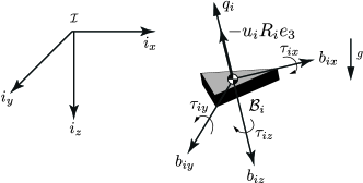
Figure 1: Vehicle class under consideration.

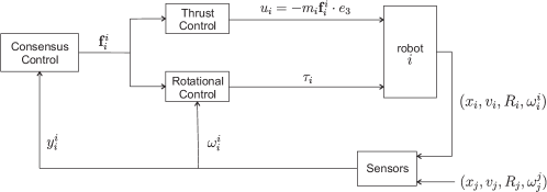
Figure 2: Block diagram of the rendezvous control system for robot $i$. The outer loop assigns a desired thrust vector $\boldsymbol{\mathbf{f}}_{i}(y_{i}^{i})$. The inner loop thrust control uses $\boldsymbol{\mathbf{f}}_{i}(y_{i}^{i})$ to assign the vehicle input $u_{i}$ while the rotational control uses $\boldsymbol{\mathbf{f}}_{i}(y_{i}^{i})$ to assign the torque input $\tau_{i}$. The vector $y_{i}^{i}$ contains the relative displacements and velocities of vehicles that robot $i$ can sense, measured in the body frame of robot $i$.

The block diagram of the proposed controller is depicted in Figure 2. There are two nested loops. The outer loop treats each robot as a point-mass driven by a force input, and produces a double-integrator consensus controller which becomes a reference input for the inner loop. The inner loop assigns local and distributed feedbacks for the robots. More intuition is provided in Section V.

Besides having a simple expression making its real-time implementation feasible, the proposed controller meets the sensing requirements of the rendezvous control problem. In particular, it does not require any knowledge of the robots’ absolute positions and velocities, or of their attitudes. It does not even require sensing of the relative attitudes. Finally, the controller does not require any communication among robots.

Our main result, Theorem 1, states that the proposed controller does indeed solve the rendezvous control problem, and in so doing it effectively reduces the problem to one of consensus for double-integrators. The latter problem has been researched extensively in the literature (e.g., [1, 2, 3]).

I-A Related work

Typical coordination problems include attitude synchronization, rendezvous, flocking, and formation control. For networks of single or double-integrator systems, the rendezvous problem is referred to as consensus or agreement, and it has been investigated by many researchers, for instance [1, 2, 3, 4, 5, 6, 7, 8].

A passivity-based solution of the attitude synchronization problem for kinematic vehicle models is proposed in [9]. In [10, 11, 12], the same problem is investigated for dynamic vehicle models. The proposed controllers do not require measurements of the angular velocity, but they do require absolute attitude measurements. In [13], the authors use the energy shaping approach to design local and distributed controllers for attitude synchronization. The same approach is adopted in [14] to design two attitude synchronization controllers, both local and distributed. The first controller achieves almost-global synchronization for directed connected graphs. However, the controller design is based on distributed observers [15], and therefore requires auxiliary states to be communicated among neighboring vehicles. It also employs an angular velocity dissipation term that forces all vehicle angular velocities to zero in steady-state. The second controller in [14] does not restrict the final angular velocities, and does not require communication, but it requires an undirected sensing graph, and guarantees only local convergence.

The rendezvous problem for kinematic unicycles was solved in [16] using time-varying feedbacks. The papers [16, 17, 18, 19] discuss the feasibility of achieving various formations using local and distributed feedback for kinematic unicycle models. Dynamic unicycle models are considered in [20, 21]. In [20], a two-mode formation control is presented in which the sensing graph has a spanning tree with a designated leader vehicle as the root. Each vehicle, however, has access to the acceleration of the leader through communication. The control strategy requires a switch between two control modes designed to deal with nonholonomic constraints in the system. The paper [21] presents a local and distributed control law making dynamic and kinematic unicycles converge to a common circle whose centre is stationary and dependent on the initial configuration of the vehicles. The spacing and ordering of unicycles on the circle is also controlled. The problem is solved using a three step hierarchical control based on a reduction theorem for the stabilization of sets.

The case of kinematic vehicles in three-space is investigated in [13, 22, 23, 24]. The authors of [13, 22] consider the problem of full attitude and position synchronization, but assume fully actuated vehicles. In [24], the authors propose distributed controllers to stabilize relative equilibria which, as shown in [25, 26], correspond to parallel, circular or helical formations. Finally, in [27, 28] the authors consider formation control for dynamic, underactuated vehicle models. However, the feedbacks are not local and distributed. Also, in [28] the sensing graph is assumed to be undirected, and communication among vehicles is required, while in [27] the graph is balanced, and it is assumed that each vehicle has access to the thrust input of its neighbors, therefore requiring once again communication between vehicles. Both approaches in [27, 28] use a two-stage backstepping methodology in which the first stage treats each vehicle as a point-mass system to which a desired thrust is assigned. A desired thrust direction is then extracted and backstepping is used to design a rotational control such that vehicle rendezvous or formation control is achieved. Our previous work [29] investigates almost-global vehicle rendezvous making use of a two-stage hierarchical methodology similar to [27, 28]. In this approach, one can combine a consensus controller for a network of double-integrators and an attitude tracking controller satisfying certain assumptions to produce a rendezvous controller for underactuated vehicles. However, this approach requires that all vehicles can sense a common inertial vector in their own body frame, which requires additional on-board sensors. Moreover, the approach requires communication among vehicles. The solution presented in this paper overcomes all these limitations. To the best of our knowledge, a solution to the rendezvous control problem for underactuated flying vehicles stated earlier has not yet appeared in the literature.

I-B Organization of the paper.

We begin, in Section II, by introducing some notation and presenting basic notions of homogeneity of functions and stability of sets. In Section III we review the vehicle model. In Section IV we formulate the rendezvous control problem. The main result, Theorem 1, is presented in Section V, and its proof in Section VI. In Section VII, we present simulation results showing that the proposed solution is robust against measurement errors, as well as force and torque disturbances. Finally, in Section VIII, we end the paper with some remarks. The proof of the main result relies on two technical lemmas that are proved in the appendix.

II Preliminaries and notation

We denote by $\mathbb{R}_{+}$ the set of positive real numbers. We use interchangeably the notation $v=[v_{1}\ \cdots\ v_{n}]^{\top}$ or $(v_{1},\ldots,v_{n})$ for a column vector in $\mathbb{R}^{n}$. We denote by ${\boldsymbol{1}}\in\mathbb{R}^{n}$ the vector $(1,\ldots,1)$. If $v,w$ are vectors in $\mathbb{R}^{3}$, we denote by $v\cdot w:=v^{\top}w$ their Euclidean inner product (also called the dot product), and by $\|v\|:=(v\cdot v)^{1/2}$ the Euclidean norm of $v$. If $v=(v_{x},v_{y},v_{z})$, we define

$$v^{\times}:=\left[\begin{array}[]{rrr}0&\ \ -v_{z}&\ \ v_{y}\\ v_{z}&\ \ 0&\ \ -v_{x}\\ -v_{y}&\ \ v_{x}&\ \ 0\end{array}\right].$$

One has that $v^{\times}w=v\times w$. Let $\{e_{1},e_{2},e_{3}\}$ denote the natural basis of $\mathbb{R}^{3}$ and $\mathsf{SO}(3):=\{M\in\mathbb{R}^{3\times 3}:M^{-1}=M{}^{\top},\det(M)=1\}$. If $\Gamma$ is a closed subset of a Riemannian manifold ${\cal X}$, and $d:{\cal X}\times{\cal X}\to[0,\infty)$ is a distance metric on ${\cal X}$, we denote by $\|\chi\|_{\Gamma}:=\inf_{\psi\in\Gamma}d(\chi,\psi)$ the point-to-set distance of $\chi\in{\cal X}$ to $\Gamma$. If $\varepsilon>0$, we let $B_{\varepsilon}(\Gamma):=\{\chi\in{\cal X}:\|\chi\|_{\Gamma}<\varepsilon\}$ and by ${\cal N}(\Gamma)$ we denote a neighborhood of $\Gamma$ in ${\cal X}$. If $A,B\subset{\cal X}$ are two sets, denote by $A\backslash B$ the set-theoretic difference of $A$ and $B$. If $I=\{i_{1},\ldots,i_{n}\}$ is an index set, the ordered list of elements $(x_{i_{1}},\ldots,x_{i_{n}})$ is denoted by $(x_{j})_{j\in I}$.

Let $U,W$ be finite-dimensional vector spaces. A function $f:U\rightarrow W$ is homogeneous if, for all $\rho>0$ and for all $x\in V$, $f(\rho x)=\rho f(x)$. A function $f:U\times V\rightarrow W$, $f(x,y)$ is homogeneous with respect to $x$ if for all $\rho>0$ and for all $(x,y)\in U\times V$, $f(\rho x,y)=\rho f(x,y)$.

The following stability definitions are taken from [30]. Let $\Sigma:\dot{\chi}=f(\chi)$ be a smooth dynamical system with state space a Riemannian manifold ${\cal X}$. Let $\phi(t,\chi_{0})$ denote its local phase flow. Let $\Gamma\subset{\cal X}$ be a closed set that is positively invariant for $\Sigma$, i.e., for all $\chi_{0}\in\Gamma$, $\phi(t,\chi_{0})\in\Gamma$ for all $t>0$ for which $\phi(t,\chi_{0})$ is defined.

Definition 1

The set $\Gamma$ is stable for $\Sigma$ if for any $\varepsilon>0$, there exists a neighborhood ${\cal N}(\Gamma)\subset{\cal X}$ such that, for all $\chi_{0}\in{\cal N}(\Gamma)$, $\phi(t,\chi_{0})\in B_{\varepsilon}(\Gamma)$, for all $t>0$ for which $\phi(t,\chi_{0})$ is defined. The set $\Gamma$ is attractive for $\Sigma$ if there exists neighborhood ${\cal N}(\Gamma)\subset{\cal X}$ such that for all $\chi_{0}\in{\cal N}(\Gamma)$, $\lim_{t\to\infty}\|\phi(t,\chi_{0})\|_{\Gamma}=0$. The domain of attraction of $\Gamma$ is the set $\{\chi_{0}\in{\cal X}:\lim_{t\to\infty}\|\phi(t,\chi_{0})\|_{\Gamma}=0\}$. The set $\Gamma$ is globally attractive for $\Sigma$ if it is attractive with domain of attraction ${\cal X}$. The set $\Gamma$ is locally asymptotically stable (LAS) for $\Sigma$ if it is stable and attractive. The set $\Gamma$ is globally asymptotically stable for $\Sigma$ if it is stable and globally attractive. $\triangle$

Now consider a dynamical system $\Sigma(k):\dot{\chi}=f(\chi,k)$, in which $k\in\mathbb{R}^{p}$ is a vector of constant parameters (typically, control gains) and $f$ is a smooth vector field with state space a Riemannian manifold.

Definition 2

The set $\Gamma$ is globally practically stable for $\Sigma(k)$ if for any $\varepsilon>0$, there exists a gain $k^{\star}$ such that $B_{\varepsilon}(\Gamma)$ has a subset which is globally asymptotically stable for $\Sigma(k^{\star})$. $\triangle$

III Modeling

We now return to the $i$-th robot depicted in Figure 1, with the aim of deriving its equations of motion. We fix a right-handed orthonormal inertial frame ${\cal I}$, common to all robots, and attach at the centre of mass of robot $i$ a right-handed orthonormal body frame ${\cal B}_{i}=\{b_{ix},b_{iy},b_{iz}\}$, as depicted in the figure. We denote by $(x_{i},v_{i})$ the inertial position and velocity of robot $i$. We let $g$ denote the gravity vector in frame ${\cal I}$.

We let $R_{i}$ be the $3\times 3$ matrix whose columns are the coordinate representations of $b_{ix},b_{iy},b_{iz}$ (in this order) in frame ${\cal I}$, so that $R_{i}\in\mathsf{SO}(3)$. The unit vector $q_{i}:=-R_{i}e_{3}$, depicted in Figure 1, is referred to as the thrust direction vector of robot $i$, and the matrix $R_{i}$ is referred to as the attitude of the robot. We assume that a thrust force $u_{i}q_{i}$ is applied at the centre of mass of robot $i$. Notice that $u_{i}q_{i}$ has magnitude $u_{i}$, is directed opposite to $b_{iz}$, and has constant direction in body frame ${\cal B}_{i}$.

Robot $i$ is assumed to have an actuation mechanism that induces control torques $\tau_{ix},\tau_{iy},\tau_{iz}$ about its body axes. We let $\tau_{i}:=(\tau_{ix},\tau_{iy},\tau_{iz})$ be the torque vector, and $\omega_{i}$ denote the angular velocity of the robot with respect to frame ${\cal I}$ (the unique vector in $\mathbb{R}^{3}$ such that $\dot{R}_{i}(R_{i})^{-1}=\omega_{i}^{\times}$).

In this paper we adopt the convention that if $r\in\mathbb{R}^{3}$ is an inertial vector, the coordinate representation of $r$ in frame ${\cal B}_{i}$ is denoted by $r^{i}$, that is, $r^{i}:=R_{i}^{-1}r$. In particular, the angular velocity of robot $i$ in its own body frame is denoted by $\omega_{i}^{i}$. Finally, we use boldface symbols to denote reference quantities. For instance, $\boldsymbol{\mathbf{f}}_{i}$ is the reference force for vehicle $i$ as in (5) and ${\boldsymbol{\boldsymbol{\omega}}}_{i}$ is the reference angular velocity for vehicle $i$ as in (9). The notation is summarized in Table I.

Picking $(x_{i},v_{i},R_{i},\omega_{i}^{i})$ as state for robot $i$, we obtain the equations of motion

$$\dot{x}_{i} =v_{i},$$ (1)

$$m_{i}\dot{v}_{i} =-u_{i}R_{i}e_{3}+m_{i}g,$$

$$\dot{R}_{i} =R_{i}\,(\omega_{i}^{i})^{\times},$$ (2)

$$J_{i}\dot{\omega}_{i}^{i} =\tau_{i}-\omega_{i}^{i}\times J_{i}\omega_{i}^{i}.$$

In the above, $m_{i}$ is the mass of robot $i$ and $J_{i}=J_{i}^{\top}$ is its inertia matrix. We define the (inertial) relative positions and velocities as $x_{ij}:=x_{j}-x_{i}$, $v_{ij}:=v_{j}-v_{i}$. This model is standard and is widely used in the literature to model flying vehicles such as quadrotor helicopters. See, for instance, [31]. Sometimes researchers use alternative attitude representations, prominently quaternions [28] or Euler angles [32, 33]. The model (1)-(2) ignores aerodynamic effects such as drag and wind disturbances (such effects are included in [31]). It also ignores the dynamics of the actuators.

TABLE I: Table of Notation

Quantity	Description
$m_{i},\ J_{i}$	mass and inertia matrix of robot $i$
$x_{i}\in\mathbb{R}^{3}$	inertial position of robot $i$
$v_{i}\in\mathbb{R}^{3}$	linear velocity of robot $i$
$R_{i}\in\mathsf{SO}(3)$	attitude of robot $i$
$\omega_{i}\in\mathbb{R}^{3}$	angular velocity of robot $i$
$q_{i}=-R_{i}e_{3}$	thrust direction vector of robot $i$
$r^{i}=R_{i}^{-1}r$	coord. repr. of $r$ in frame ${\cal B}_{i}$
$x_{ij}=x_{j}-x_{i}$	rel. displacement of robot $j$ wrt robot $i$
$v_{ij}=v_{j}-v_{i}$	rel. velocity of robot $j$ wrt robot $i$
$\boldsymbol{\mathbf{f}}_{i}\in\mathbb{R}^{3}$	reference force of robot $i$
${\boldsymbol{\boldsymbol{\omega}}}_{i}\in\mathbb{R}^{3}$	reference angular velocity of robot $i$
${\cal N}_{i}$	set of neighbors of robot $i$
$y_{i}=(x_{ij},v_{ij})_{j\in{\cal N}_{i}}$	vector of rel. pos. and vel. available to robot $i$

IV Rendezvous Control Problem

We begin by defining the sensor digraph $\mathcal{G}=(\mathcal{V},\mathcal{E})$, where $\mathcal{V}$ is a set of nodes labelled as $\{1,\dots,n\}$, each representing a robot, and $\mathcal{E}$ is the set of edges. An edge from node $i$ to node $j$ indicates that robot $i$ can sense robot $j$ (${\cal G}$ has no self-loops). A node is globally reachable if there exists a path from any other node to it .

We denote by ${\cal N}_{i}\subset{\cal V}$ the set of vehicles that robot $i$ can sense. In a realistic scenario, ${\cal N}_{i}$ is the set of robots within the field of view of robot $i$. For instance, if each robot mounted an omnidirectional camera, then one could define ${\cal N}_{i}$ to be the collection of robots that are within a given distance from robot $i$. With such a definition, the sensor digraph ${\cal G}$ would be state-dependent, making the stability analysis too hard at present.

In light of the above, in this paper we assume that ${\cal N}_{i}$ is constant for each $i\in\{1,\ldots,n\}$ (and hence ${\cal G}$ is constant as well). If $j\in{\cal N}_{i}$, then we say that robot $j$ is a neighbour of robot $i$. If this is the case, then robot $i$ can sense the relative displacement and velocity of robot $j$ in its own body frame, i.e., the quantities $x_{ij}^{i},v_{ij}^{i}$. Define the vector $y_{i}:=(x_{ij},v_{ij})_{j\in{\cal N}_{i}}$. The relative displacements and velocities available to robot $i$ are contained in the vector $y_{i}^{i}:=(x^{i}_{ij},v^{i}_{ij})_{j\in{\cal N}_{i}}$. We also assume that robot $i$ can sense its own angular velocity in its own frame ${\cal B}_{i}$. To summarize, we have the definition below.

Definition 3

A local and distributed feedback $(u_{i},\tau_{i})$ for robot $i$ is a locally Lipschitz function of $y_{i}^{i}$ and $\omega_{i}^{i}$. $\triangle$

The adjective local indicates that all quantities are represented in the body frame of robot $i$, while distributed indicates that only relative quantities with respect to neighboring robots are accessible. In applications, a local and distributed feedback for robot $i$ can be computed with on-board cameras and rate gyroscopes.

We are now ready to define the Rendezvous Control Problem.

Rendezvous Control Problem: Consider system (1), (2), and define the rendezvous manifold

$$\Gamma:= \left\{(x_{i},v_{i},R_{i},\omega_{i}^{i})_{i\in\{1,\dots,n\}}\in\mathbb{R}^{3n}\times\mathbb{R}^{3n}\times\mathsf{SO}(3)^{n}\times\mathbb{R}^{3n}\right.$$ (3)

$$:\left.x_{ij}=v_{ij}=0,\ \forall i,j\right\}.$$

Find, if possible, local and distributed feedbacks $(u_{i},\tau_{i})_{i=1,\ldots,n}$ that globally practically stabilize $\Gamma$. $\triangle$

The goal of the rendezvous control problem is to achieve synchronization of the robot positions and velocities to any desired degree of accuracy from any initial configuration.

V Solution of the Rendezvous Control Problem

Definition 4

Consider a collection of $n$ double-integrators

$$\dot{x}_{i} =v_{i}$$ (4)

$$\dot{v}_{i} =f_{i},\ i=1\dots n,$$

where $f_{i}$ is the control input of subsystem $i$. Suppose the double-integrators have the same sensor digraph ${\cal G}$ as the underactuated robots of Section III. A feedback $\boldsymbol{\mathbf{f}}_{i}(y_{i})$, $i=1\dots n$, is a double-integrator consensus controller if $\boldsymbol{\mathbf{f}}_{i}$ has the form

$$\boldsymbol{\mathbf{f}}_{i}(y_{i})=\sum_{j\in{\cal N}_{i}}\Big{(}a_{ij}x_{ij}+b_{ij}v_{ij}\Big{)},\ i=1,\ldots,n,$$ (5)

with $a_{ij},\ b_{ij}\in\mathbb{R}$ and if, setting $f_{i}=\boldsymbol{\mathbf{f}}_{i}(y_{i})$ in (4), the set

$$\left\{(x_{i},v_{i})_{i\in\{1\dots n\}}\in\mathbb{R}^{3n}\times\mathbb{R}^{3n}:x_{ij}=0,v_{ij}=0,\ \forall i,j\right\}$$

is globally asymptotically stable for (4). $\triangle$

Ren et al. in [1, Theorems 4.1, 4.2] and Yu et al. in [2, Theorem 1] have shown that a double-integrator consensus controller exists if and only if the sensor digraph ${\cal G}$ has a globally reachable node. Now the main result of this paper.

Theorem 1

If the sensor digraph ${\cal G}$ has a globally reachable node, then the rendezvous control problem is solvable for system (1)-(2), and a solution is given as follows. Let $\boldsymbol{\mathbf{f}}_{i}$, $i=1,\ldots,n$, be a double-integrator consensus controller. The local and distributed feedback,

$$\begin{split}u_{i}=&-m_{i}\boldsymbol{\mathbf{f}}_{i}(y_{i}^{i})\cdot e_{3},\\ \tau_{i}=&\omega_{i}^{i}\times J_{i}\omega_{i}^{i}-k_{1}J_{i}\left((\omega_{i}^{i}\times\boldsymbol{\mathbf{f}}_{i}(y_{i}^{i}))\times e_{3}\right)\end{split}$$ (6)

$$-k_{1}^{2}k_{2}\left[\omega_{i}^{i}-k_{1}(\boldsymbol{\mathbf{f}}_{i}(y_{i}^{i})\times e_{3})\right],\ i=1\dots n,$$

where $k_{1},k_{2}>0$ are control parameters, makes the rendezvous manifold (3) globally practically stable. In particular, for any $\varepsilon>0$, there exist $k_{1}^{\star},k_{2}^{\star}>0$ such that for all $k_{1}>k_{1}^{\star}$, $k_{2}>k_{2}^{\star}$, the set $B_{\varepsilon}(\Gamma)$ has a globally asymptotically stable subset.

The proof of Theorem 1 is presented in Section VI.

Explanation of proposed controller

Returning to the block diagram of Figure 2, we now explain in detail the operation of its two nested loops. We begin with the observation that a double-integrator consensus controller $\boldsymbol{\mathbf{f}}_{i}(y_{i})$, $i=1\dots n$, for system (4) also makes the systems

$$\dot{x}_{i} =v_{i}$$ (7)

$$\dot{v}_{i} =f_{i}+g$$

rendezvous, since the addition of the gravity vector $g$ does not affect the relative dynamics. Now compare system (7) to the translational dynamics of the flying robots,

$$\dot{x}_{i} =v_{i}$$ (8)

$$\dot{v}_{i} =-\frac{1}{m_{i}}u_{i}R_{i}e_{3}+g.$$

If it were the case that $f_{i}=-(1/m_{i})u_{i}R_{i}e_{3}$, systems (7) and (8) would be identical. Then, setting $-u_{i}R_{i}e_{3}=m_{i}\boldsymbol{\mathbf{f}}_{i}$ in (8) would solve the rendezvous problem. Inspired by this observation, the outer loop of the block diagram in Figure 2 assumes that $-u_{i}R_{i}e_{3}$ is the control input of (8) and computes a desired double-integrator force $m_{i}\boldsymbol{\mathbf{f}}_{i}$ which becomes a reference signal for the inner loop.

We now explore in more detail the operation of the inner loop. First we observe that since $\boldsymbol{\mathbf{f}}_{i}$ is a linear function, we have $R_{i}\boldsymbol{\mathbf{f}}_{i}(y_{i}^{i})=\boldsymbol{\mathbf{f}}_{i}(R_{i}y_{i}^{i})=\boldsymbol{\mathbf{f}}_{i}(y_{i})$. Moreover, using the fact that dot products are invariant under rotations, we have

$$u_{i}=-m_{i}\boldsymbol{\mathbf{f}}_{i}(y_{i}^{i})\cdot e_{3}=m_{i}(R_{i}\boldsymbol{\mathbf{f}}_{i}(y_{i}^{i}))\cdot(-R_{i}e_{3})=m_{i}\boldsymbol{\mathbf{f}}_{i}(y_{i})\cdot q_{i},$$

where $q_{i}$ is the thrust direction vector. Thus, the thrust magnitude is the projection of the desired thrust $m_{i}\boldsymbol{\mathbf{f}}_{i}$ onto the thrust direction vector—see Figure 3. Now let ${\boldsymbol{\boldsymbol{\omega}}}^{i}_{i}(y_{i}^{i})=k_{1}\left(\boldsymbol{\mathbf{f}}_{i}(y^{i}_{i})\times e_{3}\right)$. Then we have

$$\tau_{i}= \omega_{i}^{i}\times J_{i}\omega_{i}^{i}-k_{1}J_{i}\left((\omega_{i}^{i}\times\boldsymbol{\mathbf{f}}_{i}(y_{i}^{i}))\times e_{3}\right)$$ (9)

$$-k_{1}^{2}k_{2}\left(\omega_{i}^{i}-{\boldsymbol{\boldsymbol{\omega}}}_{i}^{i}(y_{i}^{i})\right).$$

We will show in the proof of Theorem 1 that the torque inputs $\tau_{i}$ make $\omega_{i}^{i}$ converge to an arbitrarily small neighborhood of ${\boldsymbol{\boldsymbol{\omega}}}_{i}^{i}$, $i=1,\ldots,n$. Thus, ${\boldsymbol{\boldsymbol{\omega}}}_{i}^{i}$ can be seen as a reference angular velocity for the inner loop. Using the fact that, for all $a,b\in\mathbb{R}^{3}$ and all $R\in\mathsf{SO}(3)$, $R(a\times b)=(Ra)\times(Rb)$, we have

$${\boldsymbol{\boldsymbol{\omega}}}_{i} =R_{i}{\boldsymbol{\boldsymbol{\omega}}}_{i}^{i}=R_{i}k_{1}\left(\boldsymbol{\mathbf{f}}_{i}(y^{i}_{i})\times e_{3}\right)=k_{1}\left((R_{i}\boldsymbol{\mathbf{f}}_{i}(y^{i}_{i}))\times(R_{i}e_{3})\right)$$

$$=k_{1}(\boldsymbol{\mathbf{f}}_{i}(y_{i})\times-q_{i})=k_{1}(q_{i}\times\boldsymbol{\mathbf{f}}_{i}(y_{i})).$$

Thus ${\boldsymbol{\boldsymbol{\omega}}}_{i}$ is perpendicular to the plane formed by the thrust direction vector $q_{i}$ and the desired thrust force $m_{i}\boldsymbol{\mathbf{f}}_{i}$—see Figure 3. Since the angular velocity vector identifies an instantaneous axis of rotation, it follows that if $\omega_{i}={\boldsymbol{\boldsymbol{\omega}}}_{i}$, then robot $i$ rotates about ${\boldsymbol{\boldsymbol{\omega}}}_{i}$ according to the right-hand rule. Referring to Figure 3, we see that such a rotation closes the gap between $u_{i}q_{i}$ and $m_{i}\boldsymbol{\mathbf{f}}_{i}$, and the speed of rotation is proportional to $\sin\varphi$, where $\varphi$ is the angle between $u_{i}q_{i}$ and $m_{i}\boldsymbol{\mathbf{f}}_{i}$ marked in the figure. When the gap is closed, we have $u_{i}=\|m_{i}\boldsymbol{\mathbf{f}}_{i}\|$, $q_{i}=m_{i}\boldsymbol{\mathbf{f}}_{i}/\|m_{i}\boldsymbol{\mathbf{f}}_{i}\|$, and thus $u_{i}q_{i}=m_{i}\boldsymbol{\mathbf{f}}_{i}$. In conclusion, the inner loop assigns $(u_{i},\tau_{i})$ to make $\omega_{i}$ approximately converge to ${\boldsymbol{\boldsymbol{\omega}}}_{i}$, so that $u_{i}q_{i}=-u_{i}R_{i}e_{3}$ approximately converges to $m_{i}\boldsymbol{\mathbf{f}}_{i}$, which is computed by the outer loop.

While the intuition behind the proposed controller is simple, the proof that the interplay between the two nested loop results in global practical stability of the rendezvous manifold is rather delicate, and it crucially relies on the homogeneity of the functions $\boldsymbol{\mathbf{f}}_{i}$, $i=1,\ldots,n$.

Remark 1

Theorem 1 proves global practical stability of the rendezvous manifold $\Gamma$. The reason that the stability is practical and not asymptotic is roughly as follows. In order to achieve rendezvous of the rigid bodies, $u_{i}q_{i}$ is driven approximately to $m_{i}\boldsymbol{\mathbf{f}}_{i}$. What’s important is not so much the difference in magnitude of these vectors but rather the difference in angle between them. In Figure 3, one can see that ${\boldsymbol{\boldsymbol{\omega}}}_{i}$ acts to reduce this angle with a rate proportional to the magnitude of ${\boldsymbol{\boldsymbol{\omega}}}_{i}$. Since ${\boldsymbol{\boldsymbol{\omega}}}_{i}$ is a linear function of $\boldsymbol{\mathbf{f}}_{i}$, as the robots approach consensus ${\boldsymbol{\boldsymbol{\omega}}}_{i}$ converges to zero at the same rate as $\boldsymbol{\mathbf{f}}_{i}$. This leads to increasing inaccuracy in closing the gap between the vectors $u_{i}q_{i}$ and $m_{i}\boldsymbol{\mathbf{f}}_{i}$ insomuch that in a very small neighborhood of rendezvous, ${\boldsymbol{\boldsymbol{\omega}}}_{i}$ is so small that it fails to make the translational dynamics act as double integrators. More detailed reasoning is provided in Remark 2.

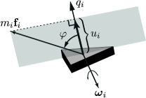
Figure 3: Illustration of the control input $u_{i}$ and reference angular velocity ${\boldsymbol{\boldsymbol{\omega}}}_{i}$ in (6).

Features of the proposed controller

(i)   The proposed controller has a number of advantages over our previous work in [29]. Unlike [29], the inner control loop does not require any derivatives of the reference thrust force $\boldsymbol{\mathbf{f}}_{i}$. In [29], the large expressions resulting from such derivatives pose difficulty in real-time computation of the control law. More importantly, the computation of such derivatives requires communication between neighboring robots, a problem that has been overcome in the present approach. The approach in [29] requires that robots have access to a common inertial vector. This requirement is absent in this paper.

(ii)   The feedback of Theorem 1 is static. It does not depend on dynamic compensators that require communication between neighboring robots.

(iii)   The feedback of Theorem 1 is local and distributed in the sense of Definition 3. Interestingly, it does not require sensing of relative attitudes, which can be computed using on-board cameras, but are harder to compute than relative displacements.

(iv)   On the rendezvous manifold $\Gamma$ there is no prespecified thrust direction $q_{i}$ for robot $i$ and the robot thrust directions do not need to align at rendezvous. This is desirable if one wants to employ the proposed controller in a hierarchical control setting to enforce additional control specifications.

VI Proof of Theorem 1

The feedback in (6) is local and distributed because it is a smooth function of $y_{i}^{i}$ and $\omega_{i}^{i}$ only. By Theorems 4.1 and 4.2 in [1] (or Theorem 1 in [2]), if ${\cal G}$ has a globally reachable node then there exists a double-integrator consensus controller, and the feedback (6) is well-defined. We need to show that it renders the rendezvous manifold $\Gamma$ in (3) globally practically stable. We begin by expressing the translational portion of the dynamics in coordinates relative to robot $1$, i.e., in terms of the variables $(x_{1j},v_{1j})_{j=2,\ldots,n}$,

$$\begin{split}\dot{x}_{1j}&=v_{1j},\\ \dot{v}_{1j}&=-\frac{1}{m_{j}}R_{j}e_{3}u_{j}+\frac{1}{m_{1}}R_{1}e_{3}u_{1},\quad j=2,\ldots,n,\\ \end{split}$$ (10)

$$\begin{split}&\dot{R}_{i}=R_{i}(\omega_{i}^{i})^{\times},\\ &J_{i}\dot{\omega}_{i}^{i}=\tau_{i}-\omega_{i}^{i}\times J_{i}\omega_{i}^{i},\quad i=1,\ldots,n.\end{split}$$ (11)

Since all relative states $(x_{ij},v_{ij})$ can be expressed in terms of the variables above through the identity $(x_{ij},v_{ij})=(x_{1j}-x_{1i},v_{1j}-v_{1i})$, perfect rendezvous occurs if and only if the vector $(x_{1j},v_{1j})_{j=2,\ldots,n}$ is zero. Denoting,

$$X:=(x_{1j},v_{1j})_{j=2,\ldots,n}\in{\sf X}:=\mathbb{R}^{3(n-1)}\times\mathbb{R}^{3(n-1)},$$

$$R:=(R_{1},\ldots,R_{n})\in{\sf R}:=\mathsf{SO}(3)^{n},$$

$$\omega:=(\omega_{1}^{1},\ldots,\omega_{n}^{n})\in{\sf\Omega}:=\mathbb{R}^{3n},$$

the new collective state is $(X,R,\omega)\in{\sf X}\times{\sf R}\times{\sf\Omega}$. The meaning of the new state is this: $X$ contains all translational states (positions and velocities) relative to robot $1$, $R$ contains all the attitudes, and $\omega$ contains all body frame angular velocities. The rendezvous manifold in new coordinates is the set $\{(X,R,\omega)\in{\sf X}\times{\sf R}\times{\sf\Omega}:X=0\}$.

Due to the identity $(x_{ij},v_{ij})=(x_{1j}-x_{1i},v_{1j}-v_{1i})$, the vector $y_{i}=(x_{ij},v_{ij})_{j\in{\cal N}_{i}}$ is a linear function of $X$ which we will denote $y_{i}=h_{i}(X)$. Similarly, the vector $y_{i}^{i}=(x_{ij}^{i},v_{ij}^{i})_{j\in{\cal N}_{i}}$ is a function of $X$ and $R$, linear with respect to $X$. We will denote this function $y_{i}^{i}=h_{i}^{i}(X,R)$.

Using the definitions above, we may now express $\boldsymbol{\mathbf{f}}_{i}^{i}(y_{i}^{i})$ and ${\boldsymbol{\boldsymbol{\omega}}}_{i}(y_{i}^{i})=k_{1}(\boldsymbol{\mathbf{f}}_{i}(y_{i}^{i})\times e_{3})$ (the latter function was discussed in Section V) in terms of states. Accordingly, we define $\boldsymbol{\mathbf{g}}_{i}:{\sf X}\to\mathbb{R}^{3}$, $\boldsymbol{\mathbf{g}}_{i}^{i}:{\sf X}\times{\sf R}\to\mathbb{R}^{3}$ and ${\boldsymbol{\boldsymbol{\omega}}}:{\sf X}\times{\sf R}\to{\sf\Omega}$ as follows:

$$\boldsymbol{\mathbf{g}}_{i}(X) :=\boldsymbol{\mathbf{f}}_{i}\circ h_{i}(X),$$ (12)

$$\boldsymbol{\mathbf{g}}_{i}^{i}(X,R) :=R_{i}^{-1}\boldsymbol{\mathbf{g}}_{i}(X)=\boldsymbol{\mathbf{f}}_{i}\circ h_{i}^{i}(X,R),$$

$${\boldsymbol{\boldsymbol{\omega}}}(X,R) :=\big{(}{\boldsymbol{\boldsymbol{\omega}}}_{i}(h_{i}^{i}(X,R))\big{)}_{i=1,\ldots,n}.$$

We remark that $\boldsymbol{\mathbf{g}}_{i}$ is linear and $\boldsymbol{\mathbf{g}}_{i}^{i}$ is linear with respect to its first argument. The second identity in the definition of $\boldsymbol{\mathbf{g}}_{i}^{i}$ is due to the linearity of $\boldsymbol{\mathbf{f}}_{i}$.

Finally, we define the rendezvous manifold in new coordinates,

$$\Gamma^{\star}:=\{(X,R,\omega)\in{\sf X}\times{\sf R}\times{\sf\Omega}:X=0\}.$$ (13)

We will prove that $\Gamma^{\star}$ is globally practically stable, which will imply that $\Gamma$ is globally practically stable as well.

VI-A Lyapunov function

Consider the $n$ double-integrators (4) with control $\boldsymbol{\mathbf{f}}_{i}$ in (5), expressed in $X$ coordinates:

$$\dot{x}_{1j} =v_{1j}$$ (14)

$$\dot{v}_{1j} =\boldsymbol{\mathbf{f}}_{j}(y_{j})-\boldsymbol{\mathbf{f}}_{1}(y_{1})=\boldsymbol{\mathbf{g}}_{j}(X)-\boldsymbol{\mathbf{g}}_{1}(X),\quad j=2,\ldots,n.$$

By Definition 4, the origin of this linear time-invariant system is globally asymptotically stable. Thus, there exists a quadratic Lyapunov function $V:{\sf X}\to\mathbb{R}$, $V(X)=X^{\top}PX$, where $P$ is a symmetric positive definite matrix, such that the derivative of $V$ along the vector field in (14) is negative definite.

Let $\mathbb{J}\in\mathbb{R}^{3n\times 3n}$ be the block-diagonal matrix with the $i$-th block equal to $J_{i}$, and consider the function $W:{\sf X}\times{\sf R}\times{\sf\Omega}\rightarrow\mathbb{R}$ defined as

$$W(X,R,\omega)=\alpha W_{{\sf tran}}(X)+W_{{\sf rot}}(X,R,\omega),$$ (15)

where $\alpha>0$ is a parameter to be assigned later and

$$W_{{\sf tran}}(X) =\sqrt{V(X)}+\frac{1}{2}V(X),$$

$$W_{{\sf rot}}(X,R,\omega)= \sum_{i=1}^{n}\boldsymbol{\mathbf{g}}_{i}^{i}(X,R)\cdot e_{3}$$

$$+\frac{1}{2}(\omega-{\boldsymbol{\boldsymbol{\omega}}}(X,R)){}^{\top}\mathbb{J}(\omega-{\boldsymbol{\boldsymbol{\omega}}}(X,R)).$$

Lemma 1

Consider the continuous function $W$ defined in (15). Then

$$\alpha^{\star}:=\sup_{(X,R)\in{\sf X}\backslash\{0\}\times{\sf R}}\sum_{i}|\boldsymbol{\mathbf{g}}_{i}^{i}(X/\sqrt{V(X)},R)\cdot e_{3}|<\infty,$$

and for all $\alpha>\alpha^{\star}$, the following properties hold:

1. $W\geq 0$ and $W^{-1}(0)\subset\Gamma^{\star}$.

2. For all $c>0$, the sublevel set $W_{c}:=\{(X,R,\omega):W(X,R,\omega)\leq c\}$ is compact.

3. For all $\varepsilon>0$, there exists $\delta>0$ such that $W_{\delta}\subset B_{\varepsilon}(\Gamma^{\star})$.

The proof is in the appendix.

From now on we assume $\alpha>\alpha^{\star}$. In light of the lemma, if we show that $W$ is nonincreasing outside a certain compact region of the state space, then all trajectories of (10)-(11) with feedback (6) are bounded, ruling out finite escape times. Moreover, in light of part (iii) of the lemma, to prove that $\Gamma^{\star}$ is practically stable it suffices to prove that for every $\delta>0$, there exists a gain vector $(k_{1},k_{2})$ such that $W_{\delta}$ is globally asymptotically stable. For this, we need to show that $W\geq\delta\implies\dot{W}<0$.

VI-B Coordinate transformation

We now construct a coordinate transformation on the translational states $X$ that leverages the homogeneity property of $\boldsymbol{\mathbf{f}}_{i}$. Return to the Lyapunov function $V(X)=X{}^{\top}PX$ associated with the double-integrator consensus controller. Since $V$ is a positive definite quadratic form, its level sets are compact and convex. Consider the level set $S_{1}:=\{X\in{\sf X}:V(X)=X^{\top}PX=1\},$ and for $\rho>0$, let $S_{\rho}$ denote the set $S_{\rho}:=\{X\in{\sf X}:X=\rho\theta,\theta\in S_{1}\}$. The sets $S_{1}$ and $S_{\rho}$ are depicted in Figure 4.

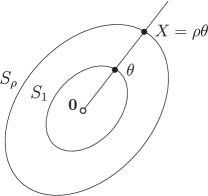
Figure 4: Illustration of the sets $S_{1}$ and $S_{\rho}$.

By convexity of $S_{1}$, any point $X\in{\sf X}\backslash\{0\}$, can be uniquely represented as $X=\rho\theta,\quad\rho\in\mathbb{R}_{+},\ \theta\in S_{1}$, where $\rho=\sqrt{X^{\top}PX}$ and $\theta=X/\rho$. In the above decomposition, one can think of $\rho$ as a scaling factor determining the size of the neighborhood of zero where $X$ belongs, while $\theta$ is a shape variable determining the relative positions and velocities of the robots modulo scaling. We use this construction to transform the coordinates of the relative translational states in $X$ as follows. Define the map

$$F:{\sf X}\backslash\{0\}\times{\sf R}\times{\sf\Omega}\to\mathbb{R}_{+}\times S_{1}\times{\sf R}\times{\sf\Omega},$$

$$F(X,R,\omega)=(\rho,\theta,R,\omega),\ \rho:=\sqrt{V(X)},\theta:=X/\sqrt{V(X)}.$$

Clearly $F$ is a smooth bijection. Moreover its inverse $F^{-1}(\rho,\theta,R,\omega)=(\rho\theta,R,\omega)$ is smooth as well, so $F$ is a diffeomorphism. The new state is $(\rho,\theta,R,\omega)\in\mathbb{R}_{+}\times S_{1}\times{\sf R}\times{\sf\Omega}$. Rendezvous in these coordinates would correspond to having $\rho=0$, which is outside of the image of $F$. This is not a problem though, since we want to show practical stability of the rendezvous manifold, for which it suffices to show that $\rho$ can be made arbitrarily small.

Having defined a coordinate transformation, our next objective is to represent the Lyapunov function candidate $W$ in new coordinates. The new representation is $\hat{W}=W\circ F^{-1}$, which amounts to simply replacing $X$ by $\rho\theta$. Doing so we obtain

$$\hat{W}(\rho,\theta,R,\omega)=\alpha\hat{W}_{\sf tran}(\rho)+\hat{W}_{\sf rot}(\rho,\theta,R,\omega),$$

where $\hat{W}_{\sf tran}(\rho)=\rho+\frac{\rho^{2}}{2}$,

$$\hat{W}_{\sf rot}(\rho,\theta,R,\omega)= \rho\sum_{i=1}^{n}\boldsymbol{\mathbf{g}}_{i}^{i}(\theta,R)\cdot e_{3}$$

$$+\frac{1}{2}\big{(}\omega-{\boldsymbol{\boldsymbol{\omega}}}(\rho\theta,R)\big{)}{}^{\top}\mathbb{J}\big{(}\omega-{\boldsymbol{\boldsymbol{\omega}}}(\rho\theta,R)\big{)}.$$

In writing the above, we used the identity $\rho=\sqrt{V(\chi)}$ and the fact that the function $\boldsymbol{\mathbf{g}}_{i}^{i}(X,R)$ is linear with respect to $X$, implying that $\boldsymbol{\mathbf{g}}_{i}^{i}(\rho\theta,R)=\rho\boldsymbol{\mathbf{g}}_{i}^{i}(\theta,R)$. In what follows, we let $\hat{W}_{\delta}:=\{(\rho,\theta,R,\omega)\in\mathbb{R}_{+}\times S_{1}\times{\sf R}\times{\sf\Omega}:\hat{W}(\rho,\theta,R,\omega)<\delta\}$. Thus, $\hat{W}_{\delta}=F(W_{\delta})$.

VI-C Stability analysis

Let $\delta>0$ be arbitrary. We have $\hat{W}\leq\alpha(\rho+\rho^{2}/2)+\rho\sup_{(\theta,R)}|\boldsymbol{\mathbf{g}}_{i}^{i}(\theta,R)\cdot e_{3}|+(1/2)(\omega-{\boldsymbol{\boldsymbol{\omega}}}){}^{\top}\mathbb{J}(\omega-{\boldsymbol{\boldsymbol{\omega}}})$. Using the definition of $\alpha^{\star}$ in Lemma 1 and the fact that $\alpha>\alpha^{\star}$, we get

$$\hat{W}\leq\alpha(2\rho+\rho^{2}/2)+(1/2)(\omega-{\boldsymbol{\boldsymbol{\omega}}}){}^{\top}\mathbb{J}(\omega-{\boldsymbol{\boldsymbol{\omega}}}).$$

It readily follows that there exists $\varrho\in(0,1)$ such that

$$\Lambda_{\varrho}:=\{(\rho,\theta,R,\omega):\rho\in(0,\varrho),\|\omega-{\boldsymbol{\boldsymbol{\omega}}}(\rho\theta,R)\|^{2}<\varrho\}\subset\hat{W}_{\delta}.$$

We will show that there exist $\alpha>0$ and a gain vector $(k_{1},k_{2})$ such that $\dot{\hat{W}}<0$ outside the set $\Lambda_{\varrho}$. This will imply that $\hat{W}\geq\delta\implies\dot{\hat{W}}<0$, proving that $\hat{W}_{\delta}$ is globally asymptotically stable.

Lemma 2

Consider the closed-loop system (10)-(11) with feedback (6). If $k_{1}>1$, then there exist scalars $M_{1},\ldots,M_{4}>0$ such that the derivatives of $\rho$ and $\hat{W}_{\sf rot}$ along the closed-loop system in $(\rho,\theta,R,\omega)$ coordinates satisfy the following inequalities:

$$\begin{split}\dot{\rho}\leq&\rho\left[-M_{2}+M_{1}\sum_{i=1}^{n}\|\boldsymbol{\mathbf{g}}_{i}^{i}(\theta,R)\times e_{3}\|\right],\\ \dot{\hat{W}}_{\sf rot}\leq&\rho^{2}\sum_{i=1}^{n}\left[-k_{1}\|\boldsymbol{\mathbf{g}}_{i}^{i}(\theta,R)\times e_{3}\|^{2}\right.\end{split}$$ (16)

$$\left.+\frac{M_{4}}{k_{2}}\right]+\rho M_{3}-\frac{k_{1}^{2}k_{2}}{2}\|\omega-{\boldsymbol{\boldsymbol{\omega}}}(\rho\theta,R)\|^{2}.$$

The proof is in the appendix.

From now on we let $k_{1}>1$. Using the inequalities in Lemma 2, we get

$$\dot{\hat{W}}\leq (\rho+\rho^{2})\left[-\alpha M_{2}+\alpha M_{1}\sum_{i=1}^{n}\|\boldsymbol{\mathbf{g}}_{i}^{i}(\theta,R)\times e_{3}\|\right]$$

$$+\rho^{2}\sum_{i=1}^{n}\left[-k_{1}\|\boldsymbol{\mathbf{g}}_{i}^{i}(\theta,R)\times e_{3}\|^{2}+\frac{M_{4}}{k_{2}}\right]$$

$$+\rho M_{3}-\frac{k_{1}^{2}k_{2}}{2}\|\omega-{\boldsymbol{\boldsymbol{\omega}}}(\rho\theta,R)\|^{2}.$$

Denote ${\boldsymbol{\beta}}_{i}(\theta,R):=\|\boldsymbol{\mathbf{g}}_{i}^{i}(\theta,R)\times e_{3}\|$, and ${\boldsymbol{\beta}}(\theta,R):=({\boldsymbol{\beta}}_{1}(\theta,R),\ldots,{\boldsymbol{\beta}}_{n}(\theta,R))$. For notational convenience, we omit the arguments of the functions ${\boldsymbol{\beta}}$ and ${\boldsymbol{\boldsymbol{\omega}}}$. With these definitions, the inequality above may be rewritten as

$$\dot{\hat{W}}\leq (\rho+\rho^{2})\left(-\alpha M_{2}+\alpha M_{1}{\boldsymbol{1}}{}^{\top}{\boldsymbol{\beta}}\right)+\rho^{2}\left(-k_{1}\|{\boldsymbol{\beta}}\|^{2}+\frac{M_{4}n}{k_{2}}\right)$$

$$+\rho M_{3}-\frac{k_{1}^{2}k_{2}}{2}\|\omega-{\boldsymbol{\boldsymbol{\omega}}}\|^{2}.$$

For every $k_{2}>nM_{4}/M_{3}$, we have

$$\dot{\hat{W}}\leq (\rho+\rho^{2})\left(-\alpha M_{2}+M_{3}+\alpha M_{1}{\boldsymbol{1}}{}^{\top}{\boldsymbol{\beta}}\right)-\rho^{2}k_{1}\|{\boldsymbol{\beta}}\|^{2}$$

$$-\frac{k_{1}^{2}k_{2}}{2}\|\omega-{\boldsymbol{\boldsymbol{\omega}}}\|^{2}.$$

If we further pick $\alpha>\max\{\alpha^{\star},3M_{3}/M_{2}\}$, we have

$$\dot{\hat{W}}\leq (\rho+\rho^{2})\left(-2M_{3}+\alpha M_{1}{\boldsymbol{1}}{}^{\top}{\boldsymbol{\beta}}\right)-\rho^{2}k_{1}\|{\boldsymbol{\beta}}\|^{2}$$

$$-\frac{k_{1}^{2}k_{2}}{2}\|\omega-{\boldsymbol{\boldsymbol{\omega}}}\|^{2}.$$

Splitting the term $-\rho^{2}k_{1}\|{\boldsymbol{\beta}}\|^{2}$ into two parts and collecting terms for $\rho$ and $\rho^{2}$, we obtain

$$\dot{\hat{W}}\leq \rho^{2}\left(-2M_{3}+\alpha M_{1}{\boldsymbol{1}}{}^{\top}{\boldsymbol{\beta}}-\frac{k_{1}}{2}\|{\boldsymbol{\beta}}\|^{2}\right)$$

$$+\rho\left(-2M_{3}+\alpha M_{1}{\boldsymbol{1}}{}^{\top}{\boldsymbol{\beta}}-\rho\frac{k_{1}}{2}\|{\boldsymbol{\beta}}\|^{2}\right)$$

$$-\frac{k_{1}^{2}k_{2}}{2}\|\omega-{\boldsymbol{\boldsymbol{\omega}}}\|^{2}.$$

Consider now the expression

$$M_{3}-\alpha M_{1}{\boldsymbol{1}}{}^{\top}{\boldsymbol{\beta}}+\frac{k_{1}\varrho}{2}\|{\boldsymbol{\beta}}\|^{2}=\big{[}{\boldsymbol{1}}{}^{\top}\ \ {\boldsymbol{\beta}}{}^{\top}\big{]}\begin{bmatrix}\frac{M_{3}}{n}I&-\alpha\frac{M_{1}}{2}I\\ -\alpha\frac{M_{1}}{2}I&\frac{k_{1}\varrho}{2}I\end{bmatrix}\begin{bmatrix}{\boldsymbol{1}}\\ {\boldsymbol{\beta}}\end{bmatrix}.$$

If $k_{1}>2n(\alpha M_{1}/2)^{2}/(\varrho M_{3})$, the above quadratic form is positive definite, implying that

$$M_{3}-\alpha M_{1}{\boldsymbol{1}}{}^{\top}{\boldsymbol{\beta}}+\frac{k_{1}\varrho}{2}\|{\boldsymbol{\beta}}\|^{2}\geq 0.$$ (17)

Since $\varrho<1$, we also have $M_{3}-\alpha M_{1}{\boldsymbol{1}}{}^{\top}{\boldsymbol{\beta}}+(k_{1}/2)\|{\boldsymbol{\beta}}\|^{2}\geq 0$. Using the latter inequality, we get a further upper bound for $\dot{\hat{W}}$,

$$\dot{\hat{W}}\leq -\rho^{2}M_{3}+\rho\left(-2M_{3}+\alpha M_{1}{\boldsymbol{1}}{}^{\top}{\boldsymbol{\beta}}-\rho\frac{k_{1}}{2}\|{\boldsymbol{\beta}}\|^{2}\right)$$ (18)

$$-\frac{k_{1}^{2}k_{2}}{2}\|\omega-{\boldsymbol{\boldsymbol{\omega}}}\|^{2}.$$

Using (18), we now prove that outside $\Lambda_{\varrho}$, $\dot{\hat{W}}<0$. In other words, when either $\rho\geq\varrho$ or $\|\omega-{\boldsymbol{\boldsymbol{\omega}}}\|^{2}\geq\varrho$, $\dot{\hat{W}}<0$.

Remark 2

If the derivative $\dot{\hat{W}}$ were negative definite, then the rendezvous manifold $\Gamma^{\star}$ would be globally asymptotically stable. However, this is not guaranteed in (18). The reason is as follows. Suppose $\rho$ is very small and $\|\omega-{\boldsymbol{\boldsymbol{\omega}}}\|=0$. Then all terms multiplied by $\rho^{2}$ become negligible and what remains in (18) is, $\dot{\hat{W}}\leq\rho\left(-2M_{3}+\alpha M_{1}{\boldsymbol{1}}{}^{\top}{\boldsymbol{\beta}}\right)$. As we have no control over the value of the constants $M_{1}$ and $M_{3}$ in the equation above, $\dot{\hat{W}}$ can be greater than zero if the second term dominates the first.

Suppose first that $\rho\geq\varrho$. Then from (18) we have

$$\dot{\hat{W}}\leq -\rho^{2}M_{3}+\rho\left(-2M_{3}+\alpha M_{1}{\boldsymbol{1}}{}^{\top}{\boldsymbol{\beta}}-\frac{k_{1}\varrho}{2}\|{\boldsymbol{\beta}}\|^{2}\right)$$

$$-\frac{k_{1}^{2}k_{2}}{2}\|\omega-{\boldsymbol{\boldsymbol{\omega}}}\|^{2}.$$

By inequality (17) we conclude that

$$\dot{\hat{W}}\leq-\rho^{2}M_{3}-\rho M_{3}-\frac{k_{1}^{2}k_{2}}{2}\|\omega-{\boldsymbol{\boldsymbol{\omega}}}\|^{2}<0.$$

Next, suppose that $\|\omega-{\boldsymbol{\boldsymbol{\omega}}}\|^{2}\geq\varrho$. Then from (18),

$$\dot{\hat{W}} \leq-\rho^{2}M_{3}+\rho\alpha M_{1}{\boldsymbol{1}}{}^{\top}{\boldsymbol{\beta}}-\frac{k_{1}^{2}k_{2}}{2}\varrho$$

$$\leq-\rho^{2}M_{3}+\rho\alpha M_{1}M_{5}-\frac{k_{1}^{2}k_{2}}{2}\varrho,$$

where $M_{5}:=\max_{(\theta,R)\in S_{1}\times{\sf R}}\{{\boldsymbol{1}}{}^{\top}{\boldsymbol{\beta}}(\theta,R)\}$. The maximum exists because ${\boldsymbol{\beta}}$ is continuous and $S_{1}\times{\sf R}$ is a compact set. If $k_{2}>(\alpha M_{1}M_{5}/k_{1})^{2}/\varrho$ then $\dot{\hat{W}}<0$.

We have therefore proved that, if $\alpha>\max\{\alpha^{\star},3M_{3}/M_{2}\}$, $k_{1}>\max\{1,2n(\alpha M_{1}/2)^{2}/(\varrho M_{3})\}$, and $k_{2}>\max\{nM_{4}/M_{3},(\alpha M_{1}M_{5}/k_{1})^{2}/\varrho\}$, then $\hat{W}>\delta$ implies that $\dot{\hat{W}}<0$. Therefore, for any initial condition, the solution of (10)-(11) with feedback (6) is bounded and the set $\hat{W}_{\delta}$ is globally asymptotically stable. $\square$

VII Simulation Results

We consider a group of five robots with the sensor digraph in Figure 5. The robot masses and inertia matrices are: $m_{1}=3$ Kg, $m_{2}=3$ Kg, $m_{3}=3.4$ Kg, $m_{4}=3.2$ Kg, $m_{5}=3.2$ Kg and $J_{1}:=\operatorname{diag}{(0.13,0.13,0.04)}$ Kg$\cdot$m², as in [28], $J_{2}=J_{1},\ J_{3}=1.4J_{1},\ J_{4}=1.2J_{1},\ J_{5}=1.2J_{1}$.

TABLE II: Simulation Initial Conditions

Vehicle $i$	$x_{i}(0)$ (m)	$v_{i}(0)$ (m/s)	$R_{i}(0)$
1	$(0,-10,10)$	$(0,0,0)$	side $1$
2	$(0,10,10)$	$(0,0,0)$	side $2$
3	$(0,0,0)$	$(0,0,0)$	down
4	$(-10,0,-10)$	$(0,0,0)$	up
5	$(10,0,-10)$	$(0,0,0)$	up

TABLE III: Control Effort

	Figure 6	Figure 7
$\max_{i}\sup_{t}|u_{i}(t)|$ (N)	20.4	17.21
$\max_{i}\sup_{t}\|\tau_{i}(t)\|$ (N$\cdot$m)	15.27	16.47
$\max_{i}\operatorname{rms}(|u_{i}(t)|)$ (N)	1.72	4.31
$\max_{i}\operatorname{rms}(\|\tau_{i}(t)\|)$ (N$\cdot$m)	1.43	2.24

We use the double-integrator consensus controller of Ren and Atkins [1], $\boldsymbol{\mathbf{f}}_{i}(y_{i})=\sum_{j=1}^{n}a_{ij}(x_{ij}+\gamma v_{ij})$ where $a_{ij}\geq 0,\ \gamma>0$. It is shown in [1] that for sufficiently large $\gamma$ the above controller does indeed achieve consensus. We pick $a_{ij}=0.3$ for all $j\in{\cal N}_{i}$ and $\gamma=30$. The control gains $k_{1}$ and $k_{2}$ in (6) are chosen to be $k_{1}=2$ and $k_{2}=0.45$. The initial conditions of the robots are shown in Table II. The initial attitudes $R_{i}(0)$ of the robots are:  up(right), side(ways) $1$, side(ways) $2$ and (upside)down respectively given by:

$$\begin{bmatrix}1&0&0\\ 0&1&0\\ 0&0&1\end{bmatrix},\ \begin{bmatrix}1&0&0\\ 0&0&-1\\ 0&1&0\end{bmatrix},\ \begin{bmatrix}1&0&0\\ 0&0&1\\ 0&-1&0\end{bmatrix},\ \begin{bmatrix}1&0&0\\ 0&-1&0\\ 0&0&-1\end{bmatrix}.$$

Figure 6 shows the simulation without the presence of disturbances while Figure 7 shows the simulation when disturbances are present. The disturbances are: an additive random noise with maximum magnitude of $0.25$ N on the applied force; an additive random noise with maximum magnitude of $0.25$ N$\cdot$m on the applied torque; an additive measurement error for the angular velocity, with maximum magnitude of $0.25$ rad/s; an additive random noise on the quantity $\boldsymbol{\mathbf{f}}_{i}(y_{i}^{i})$ accounting for errors in measurements of relative displacements and velocities of the vehicles. The direction of this vector has been rotated within $0.25$ rad and the magnitude is scaled between $0.75$ to $1.25$ times the actual magnitude. The disturbances are updated $10$ times per second. In both cases of Figure 6 and Figure 7, the vehicles’ positions and velocities converge to a neighborhood of one another.

In Figure 6 the vehicles remain within $0.25$m of one another while in Figure 7 the vehicles remain within $1$m of one another at steady state. These neighborhoods can be made even smaller by further increasing the control gains $k_{1}$ and $k_{2}$. However, this would result in having higher control inputs. Metrics related to the thrust and torque inputs are presented in Table III. The first two rows show peak control norms and the last two show the root mean square (rms) of the control norms. In these simulations we considered zero gravity, i.e., $g=0$. This was done to improve visibility of the simulation results. In the presence of gravity, the vehicles would still converge to the same neighborhood of one another, however at steady state they would accelerate in the direction of gravity since gravity is not compensated through the control inputs in (6).

Figure 5: Sensor digraph used in the simulation results.

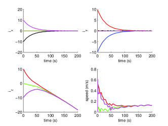
Figure 6: Rendezvous control simulation without the presence of disturbances. At the top-left, top-right and bottom-left: positions of the five robots expressed in the inertial frame ${\cal I}$. At the bottom-right: linear speeds $\|v_{i}\|,\,i=1,\dots,5$.

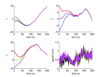
Figure 7: Rendezvous control simulation with the presence of disturbances. At the top-left, top-right and bottom-left: positions of the five robots expressed in the inertial frame ${\cal I}$. At the bottom-right: linear speeds $\|v_{i}\|,\,i=1,\dots,5$.

VIII Conclusions

We have presented the first local and distributed feedback solving the rendezvous control problem for a class of underactuated robots modelling vertical take-off and landing (VTOL) vehicles such as quadrotor helicopters. The main result, Theorem 1, relies on the assumption that the sensor digraph is constant. As we have discussed in the paper, this assumption is questionable in practice, but a stability analysis in the presence of a state-dependent sensor digraph is beyond the scope of this paper. We believe that solutions in the literature for consensus of double-integrators with time-dependent sensor digraphs could be extended to rigid bodies using the framework in this paper. However the Lyapunov function used in the analysis would need to be modified extensively. Since this makes the problem even more difficult than it already is, we leave it as a possible future research direction. In this paper we limited ourselves to the control specification of rendezvous. The proposed control law, in particular, does not guarantee hovering of the vehicles. While the robots converge to each other, nothing can be said about the motion of the ensemble. This cannot be otherwise, for it would be impossible to solve the rendezvous problem with hovering without additional sensors. One would need some measurement of the gravity vector, for example provided by a three-axis accelerometer. The point of view of these authors is that the proposed solution of the rendezvous problem will serve as a layer in a hierarchy of higher-level control specifications such as hovering, formation stabilization, and path following.

-A Proof of Lemma 1

Recall the definition of $W(X,R,\omega)$, and assume that $X\neq 0$,

$$W= \alpha\left(\sqrt{V(X)}+\frac{1}{2}V(X)\right)+\sum_{i=1}^{n}\boldsymbol{\mathbf{g}}_{i}^{i}(X,R)\cdot e_{3}$$

$$+\frac{1}{2}(\omega-{\boldsymbol{\boldsymbol{\omega}}}(X,R)){}^{\top}\mathbb{J}(\omega-{\boldsymbol{\boldsymbol{\omega}}}(X,R))$$

$$\quad= \sqrt{V(X)}\left(\alpha+\frac{\sum_{i=1}^{n}\boldsymbol{\mathbf{g}}_{i}^{i}(X,R)\cdot e_{3}}{\sqrt{V(X)}}\right)+\frac{\alpha}{2}V(X)$$

$$+\frac{1}{2}(\omega-{\boldsymbol{\boldsymbol{\omega}}}(X,R)){}^{\top}\mathbb{J}(\omega-{\boldsymbol{\boldsymbol{\omega}}}(X,R)).$$

Since $\boldsymbol{\mathbf{g}}_{i}^{i}(X,R)$ is linear with respect to $X$, we have

$$W= \sqrt{V(X)}\left(\alpha+\sum_{i=1}^{n}\boldsymbol{\mathbf{g}}_{i}^{i}\left(\mu(X),R\right)\cdot e_{3}\right)+\frac{\alpha}{2}V(X)$$

$$+\frac{1}{2}(\omega-{\boldsymbol{\boldsymbol{\omega}}}(X,R)){}^{\top}\mathbb{J}(\omega-{\boldsymbol{\boldsymbol{\omega}}}(X,R)),$$

where $\mu(X):=X/\sqrt{V(X)}$ is continuous on ${\sf X}\backslash\{0\}$ and bounded as follows

$$\|\mu(X)\|=\frac{\|X\|}{\sqrt{V(X)}}=\frac{\|X\|}{\sqrt{X{}^{\top}PX}}\leq\frac{1}{\sqrt{\lambda_{\min}(P)}}.$$

Since $\boldsymbol{\mathbf{g}}_{i}^{i}$ is continuous, $\mu(X)$ is bounded, and $R\in{\sf R}$, a compact set, it follows that the function $\sum_{i=1}^{n}\left|\boldsymbol{\mathbf{g}}_{i}^{i}\left(\mu(X),R\right)\cdot e_{3}\right|$ has a bounded supremum. Accordingly, let

$$\alpha^{\star}=\sup_{(X,R)\in{\sf X}\backslash\{0\}\times{\sf R}}\sum_{i=1}^{n}\left|\boldsymbol{\mathbf{g}}_{i}^{i}\left(\mu(X),R\right)\cdot e_{3}\right|.$$

For all $\alpha>\alpha^{\star}$, we have $W(X,R,\omega)\geq\underline{W}(X,R,\omega),$

$$\underline{W}(X,R,\omega):= \frac{\alpha}{2}V(X)$$

$$+\frac{1}{2}(\omega-{\boldsymbol{\boldsymbol{\omega}}}(X,R)){}^{\top}\mathbb{J}(\omega-{\boldsymbol{\boldsymbol{\omega}}}(X,R))\geq 0.$$

We derived the bound above for $X\neq 0$, but since $\boldsymbol{\mathbf{g}}_{i}^{i}(0,R)=0$ (by linearity of $\boldsymbol{\mathbf{g}}_{i}^{i}$ with respect to $X$), the bound also holds for $X=0$. The above inequality implies that $W\geq 0$ and $W^{-1}(0)\subset\underline{W}^{-1}(0)$. But $\underline{W}=0$ if and only if $V(X)=0$ (i.e., $X=0$) and $\omega={\boldsymbol{\boldsymbol{\omega}}}$. Thus $W^{-1}(0)\subset\Gamma^{\star}$, proving part (i) of the lemma.

For part (ii), note that for all $c>0$, $W_{c}\subset\{\underline{W}\leq c\}$. Since $\underline{W}$ is a positive definite quadratic form in the variables $(X,\omega-{\boldsymbol{\boldsymbol{\omega}}})$, its sublevel sets are compact in $(X,\omega-{\boldsymbol{\boldsymbol{\omega}}})$ coordinates. Thus if $(X,R,\omega)\in W_{c}$, $X$ and $\omega-{\boldsymbol{\boldsymbol{\omega}}}(X,R)$ are bounded. Since ${\boldsymbol{\boldsymbol{\omega}}}$ is continuous and $R\in{\sf R}$, a compact set, ${\boldsymbol{\boldsymbol{\omega}}}$ is bounded, implying that $\omega$ is also bounded. Therefore the set $W_{c}$ is bounded. Continuity of $W$ implies that $W_{c}$ is compact. This concludes the proof of part (ii) of the lemma.

For part (iii), let $\varepsilon>0$ be arbitrary. Since $\underline{W}$ is a positive definite quadratic form in the variables $(X,\omega-{\boldsymbol{\boldsymbol{\omega}}})$, there exists $\delta>0$ such that $\underline{W}(X,R,\omega)\leq\delta$ implies $\|(X,\omega-{\boldsymbol{\boldsymbol{\omega}}}(X,R))\|\leq\varepsilon$.

Furthermore, the inequality $\|(X,\omega-{\boldsymbol{\boldsymbol{\omega}}}(X,R))\|\leq\varepsilon$ implies that $\|X\|\leq\varepsilon$. Now consider any point $(X,R,\omega)\in\{\underline{W}\leq\delta\}$. We have just seen that this implies that $\|X\|\leq\varepsilon$. It will be shown next that this implies $(X,R,\omega)\in B_{\varepsilon}(\Gamma^{\star})$ and hence $\{\underline{W}\leq\delta\}\subset B_{\varepsilon}(\Gamma^{\star})$.
Note that $(X,R,\omega)\in{\sf X}\times{\sf R}\times{\sf\Omega}$ lies on the product of metric spaces ${\sf X}$, ${\sf R}$ and ${\sf\Omega}$. Respectively, the metrics are $d_{{\sf X}}$, $d_{{\sf R}}$ and $d_{{\sf\Omega}}$ ($d_{{\sf X}}$ and $d_{{\sf\Omega}}$ are Euclidean metrics). As such, choosing to use the $2$-product metric,

$$\|(X,R,\omega)\|_{\Gamma^{\star}}$$

$$=\inf_{(X_{0},R_{0},\omega_{0})\in\Gamma^{\star}}\left(d_{{\sf X}}(X,X_{0})^{2}+d_{{\sf R}}(R,R_{0})^{2}+d_{{\sf\Omega}}(\omega,\omega_{0})^{2}\right)^{\frac{1}{2}}.$$

Recall that $\Gamma^{\star}=\{(X,R,\omega)\in{\sf X}\times{\sf R}\times{\sf\Omega}:X=0\}$. As such, the point $(0,R,\omega)$ is contained in the set $\Gamma^{\star}$ and therefore,

$$\|(X,R,\omega)\|_{\Gamma^{\star}}\leq\left(d_{{\sf X}}(X,0)^{2}+d_{{\sf R}}(R,R)^{2}+d_{{\sf\Omega}}(\omega,\omega)^{2}\right)^{\frac{1}{2}}$$

where $d_{{\sf R}}(R,R)$ and $d_{{\sf\Omega}}(\omega,\omega)$ are zero. This yields, $\|(X,R,\omega)\|_{\Gamma^{\star}}\leq d_{{\sf X}}(X,0)\leq\|X\|\leq\varepsilon$. This implies that $(X,R,\omega)\in B_{\varepsilon}(\Gamma^{\star})$. Thus, $W_{\delta}\subset\{\underline{W}\leq\delta\}\subset B_{\varepsilon}(\Gamma^{\star})$, as required. This concludes the proof of Lemma 1. $\square$

-B Proof of Lemma 2

We will use a standard result from differential geometry relating the Lie derivatives of smooth functions along $F$-related vector fields [36, Proposition 8.16]. In our context, recalling that $\rho=\sqrt{V}|_{X=\rho\theta}$ and $\hat{W}=W|_{X=\rho\theta}$, the result has the following implication:

$$\dot{\rho}=\frac{d}{dt}\sqrt{V}\Big{|}_{X=\rho\theta}\text{ and }\dot{\hat{W}}_{{\sf rot}}=\frac{d}{dt}W_{\sf rot}\Big{|}_{X=\rho\theta}.$$ (19)

Rewrite the dynamics of $X$ in (10) as

$$\dot{x}_{1j} =v_{1j}$$

$$\dot{v}_{1j}= \left[\boldsymbol{\mathbf{g}}_{j}(X)-\boldsymbol{\mathbf{g}}_{1}(X)\right]$$

$$+R_{j}\left[(\boldsymbol{\mathbf{g}}_{j}^{j}(X,R)\cdot e_{3})e_{3}-\boldsymbol{\mathbf{g}}_{j}^{j}(X,R)\right]$$

$$+R_{1}\left[(\boldsymbol{\mathbf{g}}_{1}^{1}(X,R)\cdot e_{3})e_{3}-\boldsymbol{\mathbf{g}}_{1}^{1}(X,R)\right].$$

To get the identities above, we added and subtracted in (10) the ideal force feedbacks $\boldsymbol{\mathbf{f}}_{j}(y_{j})=\boldsymbol{\mathbf{g}}_{j}(X)$ and $\boldsymbol{\mathbf{f}}_{1}(y_{1})=\boldsymbol{\mathbf{g}}_{1}(X)$, and we replaced $u_{j}$ and $u_{1}$ in (10) by the assigned feedbacks in (6). Finally, we used the identity $R_{i}\boldsymbol{\mathbf{g}}_{i}^{i}=\boldsymbol{\mathbf{g}}_{i}$.

Taking the time derivative of $\sqrt{V(X)}$ along the above vector field we get

$$\frac{d}{dt}\sqrt{V(X)}= \frac{1}{2\sqrt{V(X)}}\Bigg{[}-X{}^{\top}QX$$

$$+\sum_{j=2}^{n}\frac{\partial V}{\partial v_{1j}}R_{j}\left((\boldsymbol{\mathbf{g}}_{j}^{j}(X,R)\cdot e_{3})e_{3}-\boldsymbol{\mathbf{g}}_{j}^{j}(X,R)\right)$$

$$-\sum_{j=2}^{n}\frac{\partial V}{\partial v_{1j}}R_{1}\left((\boldsymbol{\mathbf{g}}_{1}^{1}(X,R)\cdot e_{3})e_{3}-\boldsymbol{\mathbf{g}}_{1}^{1}(X,R)\right)\Bigg{]}.$$

The first term in the bracket is the derivative of $V(X)$ along the nominal vector field (14), and $Q=Q{}^{\top}$ is a positive definite matrix. Letting $M_{2}=\lambda_{\min}(Q)/(2\lambda_{\max}(P))$ and using the fact that the Euclidean norm is invariant under rotations, we have

$$\frac{d}{dt}\sqrt{V(X)}\leq -M_{2}\sqrt{V(X)}+\frac{1}{2\sqrt{V(X)}}\cdot$$

$$\Bigg{[}\sum_{j=2}^{n}\left\|\frac{\partial V}{\partial v_{1j}}\right\|\left(\|(\boldsymbol{\mathbf{g}}_{j}^{j}(X,R)\cdot e_{3})e_{3}-\boldsymbol{\mathbf{g}}_{j}^{j}(X,R)\|\right.$$

$$\left.+\|(\boldsymbol{\mathbf{g}}_{1}^{1}(X,R)\cdot e_{3})e_{3}-\boldsymbol{\mathbf{g}}_{1}^{1}(X,R)\|\right)\Bigg{]}.$$

We claim that $\|(\boldsymbol{\mathbf{g}}_{i}^{i}(X,R)\cdot e_{3})e_{3}-\boldsymbol{\mathbf{g}}_{i}^{i}(X,R)\|=\|\boldsymbol{\mathbf{g}}_{i}^{i}(X,R)\times e_{3}\|$. Indeed, writing $\boldsymbol{\mathbf{g}}_{i}^{i}=(\boldsymbol{\mathbf{g}}_{i}^{i}\cdot e_{3})e_{3}+\boldsymbol{\mathbf{g}}_{i}^{i}-(\boldsymbol{\mathbf{g}}_{i}^{i}\cdot e_{3})e_{3}$, we have $\boldsymbol{\mathbf{g}}_{i}^{i}\times e_{3}=(\boldsymbol{\mathbf{g}}_{i}^{i}-(\boldsymbol{\mathbf{g}}_{i}^{i}\cdot e_{3})e_{3})\times e_{3}$. Since the vector $\boldsymbol{\mathbf{g}}_{i}^{i}-(\boldsymbol{\mathbf{g}}_{i}^{i}\cdot e_{3})e_{3}$ is perpendicular to $e_{3}$, $\|(\boldsymbol{\mathbf{g}}_{i}^{i}-(\boldsymbol{\mathbf{g}}_{i}^{i}\cdot e_{3})e_{3})\times e_{3}\|=\|\boldsymbol{\mathbf{g}}_{i}^{i}-(\boldsymbol{\mathbf{g}}_{i}^{i}\cdot e_{3})e_{3}\|$, so that $\|\boldsymbol{\mathbf{g}}_{i}^{i}\times e_{3}\|=\|\boldsymbol{\mathbf{g}}_{i}^{i}-(\boldsymbol{\mathbf{g}}_{i}^{i}\cdot e_{3})e_{3}\|$. This proves the claim. Using the identity just derived, we get

$$\frac{d}{dt}\sqrt{V(X)}\leq -M_{2}\sqrt{V(X)}$$

$$+\frac{1}{2\sqrt{V(X)}}\Bigg{[}\sum_{j=2}^{n}\left\|\frac{\partial V}{\partial v_{1j}}\right\|\left(\|\boldsymbol{\mathbf{g}}_{j}^{j}(X,R)\times e_{3}\|\right.$$

$$\left.+\|\boldsymbol{\mathbf{g}}_{1}^{1}(X,R)\times e_{3}\|\right)\Bigg{]}.$$

Using (19), we get

$$\dot{\rho}\leq-M_{2}\rho+\frac{1}{2\rho}\Bigg{[}\sum_{j=2}^{n} \left\|\frac{\partial V}{\partial v_{1j}}(\rho\theta)\right\|\left(\|\boldsymbol{\mathbf{g}}_{j}^{j}(\rho\theta,R)\times e_{3}\|\right.$$

$$\left.+\|\boldsymbol{\mathbf{g}}_{1}^{1}(\rho\theta,R)\times e_{3}\|\right)\Bigg{]}.$$

Since the functions $\boldsymbol{\mathbf{g}}_{i}^{i}$ are linear with respect to their first argument, and the partial derivatives of the quadratic form $V$ are linear functions, by the homogeneity of the norm we have

$$\dot{\rho}\leq-M_{2}\rho+\frac{\rho}{2}\Bigg{[}\sum_{j=2}^{n} \left\|\frac{\partial V}{\partial v_{1j}}(\theta)\right\|\left(\|\boldsymbol{\mathbf{g}}_{j}^{j}(\theta,R)\times e_{3}\|\right.$$

$$\left.+\|\boldsymbol{\mathbf{g}}_{1}^{1}(\theta,R)\times e_{3}\|\right)\Bigg{]}.$$

The functions $\|\partial V/\partial v_{1j}\|$ are continuous. The variable $\theta$ belongs to $S_{1}$, a compact set. Therefore $\|\partial V/\partial v_{1j}\|$ has a maximum,

$$\dot{\rho}\leq -M_{2}\rho+\max_{\stackrel{{\scriptstyle\theta\in S_{1}}}{{j\in\{2,\ldots,n\}}}}\left\|\frac{\partial V}{\partial v_{1j}}(\theta)\right\|\frac{\rho}{2}\Bigg{[}\sum_{j=2}^{n}\left(\|\boldsymbol{\mathbf{g}}_{j}^{j}(\theta,R)\times e_{3}\|\right)$$

$$+(n-1)\|\boldsymbol{\mathbf{g}}_{1}^{1}(\theta,R)\times e_{3}\|\Bigg{]}$$

$$\leq -M_{2}\rho+\max_{\stackrel{{\scriptstyle\theta\in S_{1}}}{{j\in\{2,\ldots,n\}}}}\left\|\frac{\partial V}{\partial v_{1j}}(\theta)\right\|\frac{\rho}{2}(n-1)\sum_{j=1}^{n}\|\boldsymbol{\mathbf{g}}_{j}^{j}(\theta,R)\times e_{3}\|.$$

Letting $M_{1}:=\max_{\stackrel{{\scriptstyle\theta\in S_{1}}}{{j\in\{2,\ldots,n\}}}}\left\|\partial V/\partial v_{1j}\right\|(n-1)/2,$ we get the first inequality in (16).

We now turn to the second inequality in (16). Recall the definition of $W_{\sf rot}$,

$$W_{\sf rot}(X,R,\omega)= \sum_{i=1}^{n}\boldsymbol{\mathbf{g}}_{i}^{i}(X,R)\cdot e_{3}$$

$$+\frac{1}{2}(\omega-{\boldsymbol{\boldsymbol{\omega}}}(X,R)){}^{\top}\mathbb{J}(\omega-{\boldsymbol{\boldsymbol{\omega}}}(X,R)).$$

The time derivative of $W_{\sf rot}$ along the vector field in (10)-(11) is

$$\dot{W}_{\sf rot}=\sum_{i=1}^{n}\Bigg{[} \left(\frac{d}{dt}\boldsymbol{\mathbf{g}}_{i}^{i}\right)\cdot e_{3}+(\omega_{i}^{i}-{\boldsymbol{\boldsymbol{\omega}}}_{i}^{i}(X,R))\cdot$$

$$\left(\tau_{i}-\omega_{i}^{i}\times J_{i}\omega_{i}^{i}-J_{i}\left(\frac{d}{dt}{\boldsymbol{\boldsymbol{\omega}}}_{i}^{i}\right)\right)\Bigg{]}.$$

To express $(d/dt)\boldsymbol{\mathbf{g}}_{i}^{i}$, recall that $\boldsymbol{\mathbf{g}}_{i}^{i}(X,R)=R_{i}^{-1}\boldsymbol{\mathbf{f}}_{i}(h_{i}(X))$. Then,

$$\frac{d}{dt}\boldsymbol{\mathbf{g}}_{i}^{i}=\left(\frac{d}{dt}R_{i}^{-1}\right)\boldsymbol{\mathbf{f}}_{i}(h_{i}(X))+R_{i}^{-1}\frac{d}{dt}\left(\boldsymbol{\mathbf{f}}_{i}(h_{i}(X))\right).$$

The function $\boldsymbol{\mathbf{f}}_{i}(h_{i}(X))$ is linear. Its derivative along the vector field (10)-(11) with feedback (6) is a function of $(X,R)$ which is linear with respect to $X$ because $u_{i}=-\boldsymbol{\mathbf{g}}_{i}^{i}(X,R)\cdot e_{3}$ is such. We will denote it $\boldsymbol{\mathbf{h}}_{i}(X,R)$, $\boldsymbol{\mathbf{h}}_{i}(X,R):=(d/dt)\boldsymbol{\mathbf{f}}_{i}(h_{i}(X))$. Consistently with our notational convention in Table I, we will let $\boldsymbol{\mathbf{h}}_{i}^{i}(X,R):=R_{i}^{-1}\boldsymbol{\mathbf{h}}_{i}(X,R)$. The function $\boldsymbol{\mathbf{h}}_{i}^{i}(X,R)$ is linear with respect to $X$. Returning to the derivative of $\boldsymbol{\mathbf{g}}_{i}^{i}$, we have

$$\frac{d}{dt}\boldsymbol{\mathbf{g}}_{i}^{i} =-(\omega_{i}^{i})^{\times}R_{i}^{-1}\boldsymbol{\mathbf{f}}_{i}(h_{i}(X))+R_{i}^{-1}\boldsymbol{\mathbf{h}}_{i}(X,R)$$

$$=-\omega_{i}^{i}\times\boldsymbol{\mathbf{g}}_{i}^{i}(X,R)+\boldsymbol{\mathbf{h}}_{i}^{i}(X,R).$$

Similarly, since ${\boldsymbol{\boldsymbol{\omega}}}_{i}^{i}(X,R)=k_{1}(\boldsymbol{\mathbf{g}}_{i}^{i}(X,R)\times e_{3})$, we have $\frac{d}{dt}{\boldsymbol{\boldsymbol{\omega}}}_{i}^{i}=k_{1}\left(-\omega_{i}^{i}\times\boldsymbol{\mathbf{g}}_{i}^{i}+\boldsymbol{\mathbf{h}}_{i}^{i}\right)\times e_{3}$. Substituting the above identities in the expression for $\dot{W}_{\sf rot}$ and since $\tau_{i}=\omega_{i}^{i}\times J_{i}\omega_{i}^{i}-k_{1}J_{i}((\omega_{i}^{i}\times\boldsymbol{\mathbf{g}}_{i}^{i})\times e_{3})-k_{1}^{2}k_{2}(\omega_{i}^{i}-{\boldsymbol{\boldsymbol{\omega}}}_{i}^{i})$, we get

$$\dot{W}_{\sf rot}= \sum_{i=1}^{n}\left[-(\omega_{i}^{i}\times\boldsymbol{\mathbf{g}}_{i}^{i})\cdot e_{3}+\boldsymbol{\mathbf{h}}_{i}^{i}\cdot e_{3}\right.$$

$$\left.-k_{1}(\omega_{i}^{i}-{\boldsymbol{\boldsymbol{\omega}}}_{i}^{i})\cdot J_{i}(\boldsymbol{\mathbf{h}}_{i}^{i}\times e_{3})-k_{1}^{2}k_{2}\|\omega_{i}^{i}-{\boldsymbol{\boldsymbol{\omega}}}_{i}^{i}\|^{2}\right].$$

Using the property of the triple product that $(\omega_{i}^{i}\times\boldsymbol{\mathbf{g}}_{i}^{i})\cdot e_{3}=(\boldsymbol{\mathbf{g}}_{i}^{i}\times e_{3})\cdot\omega_{i}^{i}$, we obtain

$$\dot{W}_{\sf rot}= \sum_{i=1}^{n}\left[-(\boldsymbol{\mathbf{g}}_{i}^{i}\times e_{3})\cdot\omega_{i}^{i}+\boldsymbol{\mathbf{h}}_{i}^{i}\cdot e_{3}\right.$$

$$\left.-k_{1}(\omega_{i}^{i}-{\boldsymbol{\boldsymbol{\omega}}}_{i}^{i})\cdot J_{i}(\boldsymbol{\mathbf{h}}_{i}^{i}\times e_{3})-k_{1}^{2}k_{2}\|\omega_{i}^{i}-{\boldsymbol{\boldsymbol{\omega}}}_{i}^{i}\|^{2}\right].$$

Adding and subtracting the term $(\boldsymbol{\mathbf{g}}_{i}^{i}\times e_{3})\cdot{\boldsymbol{\boldsymbol{\omega}}}_{i}^{i}$ and collecting the term $\omega_{i}^{i}-{\boldsymbol{\boldsymbol{\omega}}}_{i}^{i}$, we have

$$\dot{W}_{\sf rot}= \sum_{i=1}^{n}\big{[}-(\boldsymbol{\mathbf{g}}_{i}^{i}\times e_{3})\cdot{\boldsymbol{\boldsymbol{\omega}}}_{i}^{i}+\boldsymbol{\mathbf{h}}_{i}^{i}\cdot e_{3}-((\boldsymbol{\mathbf{g}}_{i}^{i}\times e_{3})$$

$$+k_{1}J_{i}(\boldsymbol{\mathbf{h}}_{i}^{i}\times e_{3}))\cdot(\omega_{i}^{i}-{\boldsymbol{\boldsymbol{\omega}}}_{i}^{i})-k_{1}^{2}k_{2}\|\omega_{i}^{i}-{\boldsymbol{\boldsymbol{\omega}}}_{i}^{i}\|^{2}\big{]}.$$

Substituting in the first term inside the bracket ${\boldsymbol{\boldsymbol{\omega}}}_{i}^{i}=-k_{1}(\boldsymbol{\mathbf{g}}_{i}^{i}\times e_{3})$, taking norms, and using the fact that $k_{1}\geq 1$, we arrive at the inequality

$$\dot{W}_{\sf rot}\leq \sum_{i=1}^{n}\big{[}-k_{1}\|\boldsymbol{\mathbf{g}}_{i}^{i}\times e_{3}\|^{2}+\|\boldsymbol{\mathbf{h}}_{i}^{i}\cdot e_{3}\|$$

$$+k_{1}\boldsymbol{\mathbf{k}}_{i}(X,R)\|\omega_{i}^{i}-{\boldsymbol{\boldsymbol{\omega}}}_{i}^{i}\|-k_{1}^{2}k_{2}\|\omega_{i}^{i}-{\boldsymbol{\boldsymbol{\omega}}}_{i}^{i}\|^{2}\big{]},$$

where $\boldsymbol{\mathbf{k}}_{i}(X,R):=\|\boldsymbol{\mathbf{g}}_{i}^{i}(X,R)\times e_{3}\|+\|J_{i}(\boldsymbol{\mathbf{h}}_{i}^{i}(X,R)\times e_{3})\|$. Note that $\boldsymbol{\mathbf{k}}_{i}(X,R)$ is homogeneous with respect to $X$ because $\boldsymbol{\mathbf{g}}_{i}^{i}$ and $\boldsymbol{\mathbf{h}}_{i}$ are linear with respect to $X$ and the norm is a homogeneous function.

Splitting the term $-k_{1}^{2}k_{2}\|\omega_{i}^{i}-{\boldsymbol{\boldsymbol{\omega}}}_{i}^{i}\|^{2}$ into two parts and noticing that the function $k_{1}\boldsymbol{\mathbf{k}}_{i}(X,R)\|\omega_{i}^{i}-{\boldsymbol{\boldsymbol{\omega}}}_{i}^{i}\|-(k_{1}^{2}k_{2}/2)\|\omega_{i}^{i}-{\boldsymbol{\boldsymbol{\omega}}}_{i}^{i}\|^{2}$ is quadratic in the variable $\|\omega_{i}^{i}-{\boldsymbol{\boldsymbol{\omega}}}_{i}^{i}\|$ with maximum $\boldsymbol{\mathbf{k}}_{i}^{2}(X,R)/(2k_{2})$, we get

$$\dot{W}_{\sf rot}\leq \sum_{i=1}^{n}\bigg{[}-k_{1}\|\boldsymbol{\mathbf{g}}_{i}^{i}\times e_{3}\|^{2}+\|\boldsymbol{\mathbf{h}}_{i}^{i}\cdot e_{3}\|-\frac{k_{1}^{2}k_{2}}{2}\|\omega_{i}^{i}-{\boldsymbol{\boldsymbol{\omega}}}_{i}^{i}\|^{2}$$

$$+\frac{\boldsymbol{\mathbf{k}}_{i}^{2}(X,R)}{2k_{2}}\bigg{]}.$$

Now using (19) we get

$$\dot{\hat{W}}_{\sf rot}\leq \sum_{i=1}^{n}\bigg{[}-k_{1}\|\boldsymbol{\mathbf{g}}_{i}^{i}(\rho\theta,R)\times e_{3}\|^{2}+\|\boldsymbol{\mathbf{h}}_{i}^{i}(\rho\theta,R)\cdot e_{3}\|$$

$$-\frac{k_{1}^{2}k_{2}}{2}\|\omega_{i}^{i}-{\boldsymbol{\boldsymbol{\omega}}}_{i}^{i}\|^{2}+\frac{\boldsymbol{\mathbf{k}}_{i}^{2}(\rho\theta,R)}{2k_{2}}\bigg{]}.$$

Using the homogeneity with respect to $X$ of $\|\boldsymbol{\mathbf{g}}_{i}^{i}\times e_{3}\|$, $\|\boldsymbol{\mathbf{h}}_{i}^{i}\cdot e_{3}\|$, and $\boldsymbol{\mathbf{k}}_{i}$, we get

$$\dot{\hat{W}}_{\sf rot}\leq \sum_{i=1}^{n}\bigg{[}-k_{1}\rho^{2}\|\boldsymbol{\mathbf{g}}_{i}^{i}(\theta,R)\times e_{3}\|^{2}+\rho\|\boldsymbol{\mathbf{h}}_{i}^{i}(\theta,R)\cdot e_{3}\|$$

$$-\frac{k_{1}^{2}k_{2}}{2}\|\omega_{i}^{i}-{\boldsymbol{\boldsymbol{\omega}}}_{i}^{i}\|^{2}+\rho^{2}\frac{\boldsymbol{\mathbf{k}}_{i}^{2}(\theta,R)}{2k_{2}}\bigg{]}.$$

Since $\|\boldsymbol{\mathbf{h}}_{i}^{i}(\theta,R)\cdot e_{3}\|$ and $\boldsymbol{\mathbf{k}}_{i}^{2}(\theta,R)$ are continuous functions over the compact set $S_{1}\times{\sf R}$, they each have a maximum. Letting $M_{3}=n\cdot\max_{\stackrel{{\scriptstyle(\theta,R)\in S_{1}\times{\sf R}}}{{i\in\{1,\ldots,n\}}}}\left(\|\boldsymbol{\mathbf{h}}_{i}^{i}(\theta,R)\cdot e_{3}\|\right)$, $M_{4}=\max_{\stackrel{{\scriptstyle(\theta,R)\in S_{1}\times{\sf R}}}{{i\in\{1,\ldots,n\}}}}\left(\frac{\boldsymbol{\mathbf{k}}_{i}^{2}(\theta,R)}{2}\right),$ we conclude that

$$\dot{\hat{W}}_{\sf rot}\leq \rho^{2}\sum_{i=1}^{n}\left[-k_{1}\|\boldsymbol{\mathbf{g}}_{i}^{i}(\theta,R)\times e_{3}\|^{2}+\frac{M_{4}}{k_{2}}\right]+\rho M_{3}$$

$$-\frac{k_{1}^{2}k_{2}}{2}\sum_{i=1}^{n}\|\omega_{i}^{i}-{\boldsymbol{\boldsymbol{\omega}}}_{i}^{i}\|^{2},$$

as required. This concludes the proof of Lemma 2. $\square$

Ashton Roza received the Bachelor of Applied Science (BASc) degree in electrical engineering in 2010 from the University of Waterloo, Canada and the Master of Applied Science (MASc) from the University of Toronto, Canada, in 2012. He is currently a PhD student in the Edward S. Rogers Sr. Department of Electrical and Computer Engineering, University of Toronto, Canada. His research focuses on the application of nonlinear control and geometric methods to coordination in networks of autonomous robots.

Manfredi Maggiore was born in Genoa, Italy. He received the ”Laurea” degree in Electronic Engineering in 1996 from the University of Genoa and the PhD degree in Electrical Engineering from the Ohio State University, USA, in 2000. Since 2000 he has been with the Edward S. Rogers Sr. Department of Electrical and Computer Engineering, University of Toronto, Canada, where he is currently Professor. He has been a visiting Professor at the University of Bologna (2007-2008), and the Laboratoire des Signaux et Systèmes, Ecole CentraleSupélec (2015-2016). His research focuses on mathematical nonlinear control, and relies on methods from dynamical systems theory and differential geometry.

Luca Scardovi (M ’06) received the Laurea degree and Ph.D. degree in Electronic and Computer Engineering from the University of Genoa, Italy, in 2001 and 2005 respectively. In 2005 he was an Adjunct Professor at the University of Salento, Lecce, Italy. He held research associate positions at the Department of Electrical Engineering and Computer Science at the University of Liège, Belgium (2005-2007) and at the Department of Mechanical and Aerospace Engineering at Princeton University (2007-2009). From 2009 to 2011 he was an Assistant Professor at the Technische Universität München (TUM), Munich, Germany. He is currently an Assistant Professor in the Edward S. Rogers Sr. Department of Electrical and Computer Engineering at the University of Toronto. His research interests focus on dynamical systems with special emphasis in the analysis and control of emergent dynamics in networked dynamical systems. He is an associate editor for the IEEE Control Systems Society Conference Editorial Board and for the journal Systems & Control Letters.

References

- [1] W. Ren and E. Atkins, “Distributed multi-vehicle coordinated control via local information exchange,” International Journal of Robust and Nonlinear Control, vol. 17, pp. 1002–1033, 2007.
- [2] W. Yu, G. Chen, and M. Cao, “Some necessary and sufficient conditions for second-order consensus in multi-agent dynamical systems,” Automatica, vol. 46, no. 6, pp. 1089–1095, 2010.
- [3] T. Xia and L. Scardovi, “Synchronization Conditions for Diffusively Coupled Linear Systems,” in 21st International Symposium on Mathematical Theory of Networks and Systems, 2014, pp. 1070–1075.
- [4] W. Ren and R. Beard, “Consensus seeking in multiagent systems under dynamically changing interaction topologies,” IEEE Transactions on Automatic Control, vol. 50, no. 5, pp. 655–661, 2005.
- [5] L. Moreau, “Stability of continuous-time distributed consensus algorithms,” in Proceedings of the 43rd IEEE Conference on Decision and Control, 2004.
- [6] R. Olfati-Saber and R. Murray, “Consensus problems in networks of agents with switching topology and time-delays,” IEEE Transactions on Automatic Control, vol. 49, no. 9, pp. 1520–1533, 2004.
- [7] D. Lee and M. Spong, “Stable flocking of multiple inertial agents on balanced graphs,” IEEE Transactions on Automatic Control, vol. 52, no. 8, pp. 1469–1475, 2007.
- [8] L. Scardovi and R. Sepulchre, “Synchronization in networks of identical linear systems,” Automatica, vol. 45, no. 11, pp. 2557–2562, 2009.
- [9] T. Hatanaka, N. Chopra, M. Fujita, and M. Spong, Passivity-Based Control and Estimation in Networked Robotics. Springer International Publishing, 2015.
- [10] W. Ren, “Distributed cooperative attitude synchronization and tracking for multiple rigid bodies,” IEEE Transactions on Control Systems Technology, vol. 18, no. 2, pp. 383–392, 2010.
- [11] A. Abdessameud and A. Tayebi, “Attitude synchronization of a group of spacecraft without velocity measurements,” IEEE Transactions on Automatic Control, vol. 54, no. 11, pp. 2642–2648, 2009.
- [12] ——, Motion Coordination for VTOL Unmanned Aerial Vehicles. Springer International Publishing, 2013.
- [13] S. Nair and N. Leonard, “Stable synchronization of rigid body networks,” Networks and Heterogeneous Media, vol. 2, no. 4, pp. 595–624, 2007.
- [14] A. Sarlette, R. Sepulchre, and N. Leonard, “Autonomous rigid body attitude synchronization,” Automatica, vol. 45, pp. 572–577, 2009.
- [15] L. Scardovi, A. Sarlette, and R. Sepulchre, “Synchronization and balancing on the N-torus,” Systems & Control Letters, vol. 56, no. 5, pp. 335–341, 2007.
- [16] Z. Lin, B. Francis, and M. Maggiore, “Necessary and sufficient conditions for formation control of unicycles,” IEEE Transactions on Automatic Control, vol. 50, no. 1, pp. 121–127, 2005.
- [17] R. Sepulchre, D. Paley, and N. Leonard, “Stabilization of planar collective motion: All-to-all communication,” IEEE Trans. on Automatic Control, vol. 52, no. 5, pp. 811–824, 2007.
- [18] P. Tabuada, G. Pappas, and P. Lima, “Motion feasibility of multi-agent formations,” IEEE Trans. on Robotics, vol. 21, no. 3, pp. 387–392, 2005.
- [19] L. Consolini, F. Morbidi, D. Prattichizzo, and M. Tosques, “On a class of hierarchical formations of unicycles and their internal dynamics,” IEEE Transactions on Automatic Control, vol. 57, no. 4, pp. 845–859, 2012.
- [20] T. Liu and Z. Jiang, “Distributed formation control of nonholonomic mobile robots without global position measurements,” Automatica, vol. 49, no. 2, pp. 592–600, 2013.
- [21] M. El-Hawwary and M. Maggiore, “Distributed circular formation stabilization for dynamic unicycles,” IEEE Transactions on Automatic Control, vol. 58, no. 1, pp. 149–162, 2013.
- [22] R. Dong and Z. Geng, “Consensus based formation control laws for systems on Lie groups,” System & Control Letters, vol. 62, no. 2, pp. 104–111, 2013.
- [23] T. Hatanaka, Y. Igarashi, M. Fujita, and M. W. Spong, “Passivity-based pose synchronization in three dimensions,” IEEE Trans. on Automatic Control, vol. 57, no. 2, pp. 360–375, 2012.
- [24] L. Scardovi, N. Leonard, and R. Sepulchre, “Stabilization of collective motion in three dimensions,” Communications in information and systems, vol. 8, no. 3, pp. 473–500, 2008.
- [25] E. W. Justh and P. S. Krishnaprasad, “Equilibria and steering laws for planar formations,” Systems & Control Letters, vol. 52, no. 1, pp. 25–38, 2004.
- [26] E. Justh and P. Krishnaprasad, “Natural frames and interacting particles in three dimensions,” in 44th IEEE Conference on Decision and Control, 2005, pp. 2841–2846.
- [27] D. Lee, “Distributed backstepping control of multiple thrust-propelled vehicles on a balanced graph,” Automatica, vol. 48, no. 11, pp. 2971–2977, 2012.
- [28] A. Abdessameud and A. Tayebi, “Formation control of VTOL unmanned aerial vehicles with communication delays,” Automatica, vol. 47, no. 11, pp. 2383–2394, 2011.
- [29] A. Roza, M. Maggiore, and L. Scardovi, “A class of rendezvous controllers for underactuated thrust-propelled rigid bodies,” in Proceedings of the 53rd IEEE Conference on Decision and Control, Los Angeles, California, 2014.
- [30] M. El-Hawwary and M. Maggiore, “Reduction theorems for stability of closed sets with application to backstepping control design,” Automatica, vol. 49, no. 1, pp. 214–222, 2013.
- [31] M. Hua, T. Hamel, P. Morin, and C. Samso, “A control approach for thrust-propelled underactuated vehicles and its application to VTOL drones,” IEEE Transactions on Automatic Control, vol. 54, no. 8, pp. 1837–1853, 2009.
- [32] A. Mokhtari, A. Benallegue, and Y. Orlov, “Exact linearization and sliding mode observer for a quadrotor unmanned arial vehicle,” International Journal of Robotics and Automation, vol. 21, no. 1, pp. 39–49, 2006.
- [33] P. Castillo, R. Lozano, and A. Dzul, “Stabilization of a mini rotorcraft with four rotors,” IEEE Control Systems Magazine, pp. 45–55, 2005.
- [34] Z. Lin, B. A. Francis, and M. Maggiore, “State agreement for coupled nonlinear systems with time-varying interaction,” SIAM Journal on Control and Optimization, pp. 288–307, 2007.
- [35] H. Ando, Y. Oasa, I. Suzuki, and M. Yamashita, “Distributed memoryless point convergence algorithm for mobile robots with limited visibility,” IEEE Trans. on Robotics and Automation, pp. 818–828, 1999.
- [36] J. Lee, Introduction to Smooth Manifolds, 2nd ed. Springer, 2013.