Control and controllability of nonlinear dynamical networks: a geometrical approach

Abstract

In spite of the recent interest and advances in linear controllability of complex networks, controlling nonlinear network dynamics remains to be an outstanding problem. we develop an experimentally feasible control framework for nonlinear dynamical networks that exhibit multistability (multiple coexisting final states or attractors), which are representative of, e.g., gene regulatory networks (GRNs). The control objective is to apply parameter perturbation to drive the system from one attractor to another, assuming that the former is undesired and the latter is desired. To make our framework practically useful, we consider restricted parameter perturbation by imposing the following two constraints: (a) it must be experimentally realizable and (b) it is applied only temporarily. We introduce the concept of attractor network, in which the nodes are the distinct attractors of the system, and there is a directional link from one attractor to another if the system can be driven from the former to the latter using restricted control perturbation. Introduction of the attractor network allows us to formulate a controllability framework for nonlinear dynamical networks: a network is more controllable if the underlying attractor network is more strongly connected, which can be quantified. We demonstrate our control framework using examples from various models of experimental GRNs. A finding is that, due to nonlinearity, noise can counter-intuitively facilitate control of the network dynamics.

An outstanding problem in interdisciplinary research is to control nonlinear dynamics on complex networks. Indeed, the physical world in which we live is nonlinear, and complex networks are ubiquitous in a variety of natural, social, economical, and man-made systems. Dynamical processes on complex networks are thus expected to be generically nonlinear. While the ultimate goal to study complex systems is to control them, the coupling between nonlinear dynamics and complex network structures presents tremendous challenges to our ability to formulate effective control methodologies. In spite of the rapid development of network science and engineering toward understanding, analyzing and predicting the dynamics of large complex network systems in the past fifteen years, the problem of controlling nonlinear dynamical networks has remained open.

In the past several years, a framework for determining the linear controllability of network based on traditional control and graph theories emerged LH:2007 ; LCWX:2008 ; RJME:2009 ; LSB:2011 ; WNLG:2011 ; YZDWL:2013 ; CWWL:2015 ; NA:2012 ; YRLLL:2012 ; NV:2012 ; LSBA:2013 ; MDB:2014 ; RR:2014 ; Wuchty:2014 ; WBSS:2015 ; YTBSLB:2015 , leading to a quantitative understanding of the effect of network structure on its controllability. In particular, a structural-controllability framework was proposed LSB:2011 , revealing that the ability to steer a complex network toward any desired state, as measured by the minimum number of driver nodes, is determined by the set of maximum matching, which is the maximum set of links that do not share starting or ending nodes. A main result was that the number of driver nodes required for full control is determined by the network’s degree distribution LSB:2011 . The framework was established for weighted and directed networks. An alternative framework, the exact-controllability framework, was subsequently formulated YZDWL:2013 , which was based on the principle of maximum multiplicity to identify the minimum set of driver nodes required to achieve full control of networks with arbitrary structures and link-weight distributions. Generally, the deficiency of such rigorous mathematical frameworks of controllability is that the nodal dynamical processes must be assumed to be linear. For nonlinear nodal dynamics, the mathematical framework on which the controllability theories based, namely the classic Kalman’s controllability rank condition Kalman:1963 ; Lin:1974 ; Luenberger:book , is not applicable. At the present there is no known theoretical framework for controlling nonlinear dynamics on complex networks.

Due to the high dimensionality of nonlinear dynamical networks and the rich variety of behaviors that they can exhibit, it may be prohibitively difficult to develop a control framework that is universally applicable to different kinds of network dynamics. In particular, the classic definition of linear controllability, i.e., a network system is controllable if it can be driven from an arbitrary initial state to an arbitrary final state in finite time, is generally not applicable to nonlinear dynamical networks. Instead, controlling collective dynamical behaviors may be more pertinent and realistic WC:2002 ; LWC:2004 ; SBGC:2007 ; CZL:2014 . Our viewpoint is that, for nonlinear dynamical networks, control strategies may need to be specific and system dependent. The purpose of this paper is to articulate control strategies and develop controllability framework for nonlinear networks that exhibit multistability. A defining characteristic of such systems is that, for a realistic parameter setting, there are multiple coexisting attractors in the phase space GMOY:1983 ; MGOY:1985 ; FG:1997 ; FG:2003 ; LT:book ; NYLDG:2013 . The goal is to drive the system from one attractor to another using physically meaningful, temporary and finite parameter perturbations, assuming that the system is likely to evolve into an undesired state (attractor) or the system is already in such a state, and one wishes to implement control to bring the system out of the undesired state and steer it into a desired one. We note that dynamical systems with multistability are ubiquitous in the real world ranging from biological and ecological to physical systems Alley:2003 ; May:1977 ; SPD:2005 ; Chase:2003 ; BM:2005 ; WZXW:2011 ; HGME:2007 .

In biology, nonlinear dynamical networks with multiple attractors have been employed to understand fundamental phenomena such as cancer mechanisms Huang:2013 , cell fate differentiation SGLE:2006 ; HEYI:2005 ; FK:2012 ; LZW:2014 , and cell cycle control YTWNJY:2011 ; BT:2004 . For example, boolean network models were used to study the gene evolution KPST:2004 , attractor number variation with asynchronous stochastic updating GD:2005 , gene expression in the state space HEYI:2005 , and organism system growth rate improvement MGAB:2008 . Another approach is to abstract key regulation genetic networks MTELT:2009 ; Faucon:2014 (or motifs) from all associated interactions, and to employ synthetic biology to modify, control and finally understand the biological mechanisms within these complicated systems YTWNJY:2011 ; SGLE:2006 . An earlier application of this approach led to a good understanding of the ubiquitous phenomenon of bistability in biological systems Gardner:2000 , where there are typically limit cycle attractors and, during cell cycle control, noise can trigger a differentiation process by driving the system from a limit circle to another steady state attractor SGLE:2006 . Generally speaking, there are two candidate mechanisms for transition or switching between different attractors FK:2012 : through signals transmitted between cells and through noise, which were demonstrated recently using synthetic genetic circuits WSLELW:2013 ; WMX:2014 . More recently, a detailed numerical study was carried out of how signal-induced bifurcations in a tri-stable genetic circuit can lead to transitions among different cell types LZW:2014 .

In this paper, we develop a controllability framework for nonlinear dynamical networks based on the concept of attractor networks Lai:2014 . An attractor network is defined in the phase space of the underlying nonlinear system, in which each node represents an attractor and a directed edge from one node to another indicates that the system can be driven from the former to the latter using experimentally feasible, temporary, and finite parameter changes. A well connected attractor network implies a strong feasibility that the system can be controlled to reach a desired attractor. The connectivity of the attractor network can then be used to characterize the controllability of the nonlinear network. More specifically, for a given pair of attractors, the weighted shortest path between them in the attractor network is an indicator of the physical feasibility of the associated transition. We use gene regulatory networks (GRNs) to demonstrate our control framework, which includes low-dimensional, experimentally realizable synthetic gene circuits and a realistic T-cell cancer network of 60 nodes. A finding is that noise can counter-intuitively enhance the controllability of a nonlinear dynamical network. We emphasize that the development of our nonlinear control framework is based entirely on physical considerations, rendering feasible experimental verification.

Results

A complex, nonlinear dynamical network of $N$ variables can be described by a set of $N$ coupled differential equations:

$$\dot{\mathbf{x}}=\mathbf{F}(\mathbf{x},{\bf\mu}),$$ (1)

where $\mathbf{x}\in\mathbf{R}^{N}$ denotes the $N$-dimensional state variable, $\mathbf{F}(\mathbf{x},{\bf\mu})$ is the nonlinear vector field, and ${\bf\mu}\in\mathbf{R}^{M}$ represents the set of coupling parameters. In a GRN, the nodal dynamics is typically one dimensional. For simplicity, we assume that this is the case to be treated so that the size of the network represented by Eq. (1) is $N$. From consideration of realistic GRNs, we assume that the coupling parameters can be adjusted externally, which are effectively the set of control parameters. Specifically, in a GRN, the various coupling strengths among the nodes (genes) can be experimentally and systematically varied through application of specific targeted drugs. At a larger scale, the fate of a cell can be controlled by adding drugs to the cell-growth environment, which adjust the interaction parameters in the underlying network Gardner:2000 . While dynamical variables themselves can also be perturbed for the purpose of control, for GRNs this is unrealistic. For this reason the scenario of perturbing dynamical variables will not be considered in this paper.

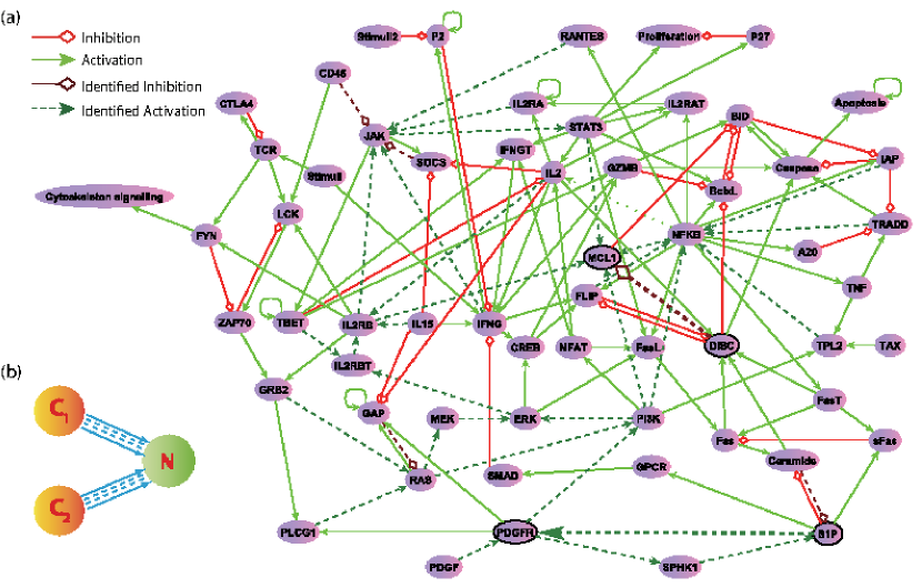
Figure 1: T-LGL survival signaling system and its attractor network. (a) Structure of T-LGL signaling network: each node is labeled with its generic name, and the arrowhead and diamond-head edges represent excitation and inhibition regulations, respectively. The inhibitory edges from “Apoptosis” to other nodes are not shown (for clarity). (b) Attractor network of the T-cell network, which contains three nodes: two cancerous states denoted as $\mathbf{C}_{1}$ and $\mathbf{C}_{2}$ and a normal state denoted as $\mathbf{N}$. Our detailed computations reveal that parameter perturbations on $48$ edges can drive the system from a cancerous state to the normal state, which are indicated with dark dashed lines, whereas the remaining edges in the network are specified with light solid lines. The two directed edges in the attractor network are multiple, containing altogether $48$ individual edges corresponding to controlling the $48$ solid-line edges in the original network.

We focus on nonlinear dynamical networks with multiple coexisting attractors. For a given set of parameters ${\bf\mu}$, the multiple attractors (e.g., stable steady states) and the corresponding basins are fixed. For a given initial condition, the system will approach one of the attractors. Each attractor has specific biological significance, which can be regarded as either desired or undesired, depending on the particular function of interest. Suppose, without any control, the system is in an undesired attractor or is in its basin of attraction. The question is how to steer the system from the undesired state to a desired state by means of temporal and small parameter variations that are experimentally feasible.

Control principle based on bifurcation.

To motivate the development of a feasible control principle, we consider the simple case where the system is near a bifurcation and control is to be applied to drive the system from one attractor to another through temporal perturbation to a single parameter. That is, the parameter variation is turned on and takes effect for a finite (typically short) duration of time. After control perturbation is withdrawn, the system is restored to its parameter setting before control but its state has been changed: it will be in the desired attractor. Let $\mu_{0}$ be the initial parameter value and the system is in an undesired attractor denoted as $\mathbf{x}_{i}^{\ast}$, and let $\mathbf{x}_{f}^{\ast}$ be the desired attractor that the system is driven to. Imposing control means that we change the parameter from $\mu_{0}$ to $\mu_{1}$. The dynamical mechanism to drive the system out of the initial attractor is bifurcations, e.g., a saddle-node bifurcation at which the original attractor disappears and its basin is absorbed into that of an intermediate attractor BT:2004 , denoted as ${\mathbf{\bar{x}}}_{k}^{\ast}$. Turning on control to change $\mu$ from $\mu_{0}$ to $\mu_{1}$ thus makes the system approach ${\mathbf{\bar{x}}}_{k}^{\ast}$. This process continues until the system falls into the original basin of $\mathbf{x}_{f}^{\ast}$, at which point the control parameter is reset to its original value $\mu_{0}$ so that the system will approach the desired attractor $\mathbf{x}_{f}^{\ast}$. Success of control relies on the existence of a “path” from the initial attractor to the final one through a number of intermediate attractors. If a single parameter is unable to establish such a path, variations in multiple parameters can be considered, provided that such parameter adjustments are experimentally realizable. For a biological network, this can be achieved through application of a combined set of drugs Feala:2010 ; Fitzgerald:2006 . However, even when potential complications induced by inter-drug interactions are neglected, the search space for suitable parameter perturbation can be prohibitively large if we allow all available parameters to be adjusted simultaneously. We demonstrate below that this challenge can be met by constructing an attractor network for the underlying system.

Attractor networks: an example of T-cell network

For a complex, nonlinear dynamical network, an attractor network can be constructed by defining each of all possible attractors of the system as a node. There exists a directed link from one node to another if an experimentally accessible parameter of the system can be adjusted to drive or control the system from the former to the latter. There can be multiple edges from one node to another, if there are multiple parameters, each enabling control. Starting from an initial attractor, one can identify, using all accessible parameters with variations in physically reasonable ranges, a set of attractors that the system can be driven into. Repeating this procedure for all attractors in the system, we build up an attractor network that provides a blueprint for driving the whole networked system from any attractor to any other attractor in the system, assuming at the time the latter attractor would lead to desired function of the system as a whole. All these can be done using relatively small parameter perturbations.

To demonstrate the construction of an attractor network, we take as an example a realistic biological network, T-cell in large granular lymphocyte leukemia associated with blood cancer. Specifically, apoptosis signaling of the T-cell can be described by a network model: T-cell survival signaling network Zhang:2008 ; Saadatpour:2011 , which has 60 nodes and 142 regulatory edges, as shown in Fig. 1(a). Nodes in the network represent proteins and transcripts, and the edges correspond to either activation or inhibitory regulations. Experimentally, it was found that there are three attractors for this biophysically detailed network Zhang:2008 ; Saadatpour:2011 . Among the three attractors, two correspond to two distinct cancerous states (denoted as $\mathbf{C}_{1}$ and $\mathbf{C}_{2}$) and one is associated with a normal state (denoted as $\mathbf{N}$). By translating the Boolean rules into a continuous form using the method in Wittmann:2009 ; KPWT:2010 and setting the strength of each edge to unity, one can obtain a set of nonlinear dynamical equations for the entire network system. Direct simulation of the model revealed that there are three stable fixed point attractors, in agreement with the experimental observation Zhang:2008 ; Saadatpour:2011 . The attractor network is thus quite simple: it has three nodes only, as shown in Fig. 1(b). Testing all experimentally adjustable parameters, we find multiple edges from each cancerous attractor to the normal one (see Supplementary Table 1). Since the goal of control is to bring the system from one of the cancerous states to the normal one, it is not necessary (or biologically meaningful) to test whether parameter perturbation exists that drives the system from the normal node to a cancerous node.

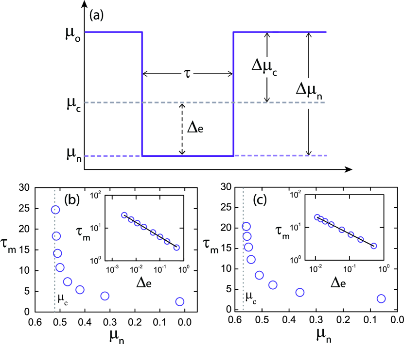
Figure 2: Relationship between edge control strength and minimal control time. For the T-cell network, (a) an inverted rectangular control signal of duration $\tau$ and amplitude $\Delta\mu=|\mu_{n}-\mu_{0}|$, where $\mu_{0}$ is the original parameter value. A saddle-node bifurcation occurs for $\mu=\mu_{c}$, so $\Delta e=\mu_{c}-\mu_{n}$ is the excess amount of the parameter change over the critical value $\mu_{c}$. (b,c) Minimal control time $\tau_{m}$ versus $\mu_{n}$, where parameter control is applied to the activation edge from node “S1P” to node “PDGFR” and to the inhibitory edge from “DISC” to “MCL1”, respectively. These four nodes are indicated using solid black circles in Fig. 1(a). The corresponding plots on a logarithmic scale in the insets of (b) and (c) suggest a power-law scaling behavior between $\tau_{m}$ and $\Delta e$ [Eq. (2)]. The fitted power-law scaling exponents are $\beta\approx 0.42$, and $0.38$, respectively, for (b) and (c).

Control implementation based on attractor network.

Given a nonlinear dynamical network in the real (physical) space, the underlying phase space dimension may be quite high, rendering analysis of the dynamical behaviors difficult. The attractor network is a coarse grained representation of the phase space, retaining information that is most relevant to the control task of driving the network system to a desired final state. Once an attractor network has been constructed, actual control can be carried out through temporary changes in a set of experimentally adjustable parameters, one at a time. This should be contrasted to one existing approach CKM:2013 that requires accurate adjustments in the state variables, which may not always be realistic.

We detail how actual control can be implemented based on the attractor network for the T-cell network. To be concrete, we assume that the control signal has the shape of a rectangular pulse in the plot of a parameter versus the time, as shown in Fig. 2(a), where the control parameter is $\mu$ and the rectangular pulse has duration $\tau$ and amplitude $\Delta\mu=|\mu_{n}-\mu_{0}|$, with $\mu_{0}$ denoting the nominal parameter value and $\mu_{n}$ being the value during the time interval when control is on. For the T-cell network, we set $\mu_{0}=1.0$. As $\mu$ is reduced the system approaches a bifurcation point. (In other examples a bifurcation can be reached by increasing a control parameter, as in low-dimensional GRNs detailed in Control Analysis.) Extensive numerical simulations in controlling the T-cell network from a cancerous state ($\mathbf{C}_{1}$ or $\mathbf{C}_{2}$) to the normal state $\mathbf{N}$ shows that, to achieve control, there are wide ranges of choices for $\Delta\mu$ and $\tau$. In fact, once $\mu_{n}$ is decreased through the bifurcation point $\mu_{c}$ at which the initial attractor loses its stability, the goal of control can be realized. The critical value $\mu_{c}$ for each parameter can be identified from a bifurcation analysis. Additionally, for $\mu_{n}<\mu_{c}$, there exists a required minimum control time $\tau_{m}$, over which the system will move into the original basin of the target attractor before control is activated. Insofar as $\tau>\tau_{m}$, the control signal can be released. Longer duration of control is not necessary since the system will evolve into the target attractor following its natural dynamical evolution associated with the nominal parameter $\mu_{0}$. The value of $\tau_{m}$ increases as $\mu_{n}$ is closer to $\mu_{c}$, where if $\mu_{n}=\mu_{c}$, $\tau_{m}$ is infinite due to the critical slowing down at the bifurcation point $\mu_{c}$. Figures 2(b) and 2(c) show, respectively, for the T-cell network, the relationship between $\tau_{m}$ and $\mu_{n}$ in controlling the strength of the activation edge from node “S1P” to node “PDGFR”, and that of the inhibitory edge from node “DISC” to node “MCL1” [cf., Fig. 1(a), the nodes denoted as black circles and connected by bold coupling edges]. The critical value $\mu_{c}$ (indicated by the dotted line) can be estimated accordingly. The insets of (b) and (c) show the corresponding plots of the relationships on a double logarithmic scale, with the horizontal axis to be $\Delta_{\mathrm{e}}=\mu_{c}-\mu_{n}$, the exceeded value of $\mu_{n}$ over the critical point $\mu_{c}$. We observe the following power-law scaling behavior:

$$\tau_{m}=\alpha|\mu_{n}-\mu_{c}|^{\beta},$$ (2)

where $\beta$ is the scaling exponent. The region of control parameters at the upper-right region over the curve of $\tau_{m}(\Delta e)$, i.e., larger $\Delta e$ value or longer duration $\tau$, corresponds to the case where control is successful in the sense that the system can definitely be driven to the desired final state.

The power-law scaling relation for $\tau_{m}$ demonstrated in Figs. 2(b) and 2(c) for the T-cell network is quite general, as it also holds for two-node and three-node GRNs (see Control Analysis). For the T-cell system, the critical values of parameters for all the possible controllable edges from $\mathbf{C}_{1}$ or $\mathbf{C}_{2}$ to $\mathbf{N}$, and the corresponding values of $\alpha$ and $\beta$ in Eq. (2) are provided in Table S1 in Supplemental Information). The control magnitude and time for some parameters are identical, for the reason that the logic relationship from the corresponding edges to the same node can be described as “AND” (c.f., Fig. 1) so that in the continuous-time differential equation model, all these in-edges are equivalent. (The control results from the two-node and three-node GRNs between any pair of nearest-neighbor attractors are listed in Tables S2 and S3 in SI, respectively.) Due to the flexibility in choosing the control signal, our control scheme based on the attractor network is amenable to experimental implementation.

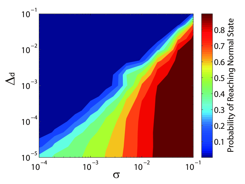
Figure 3: Beneficial role of noise in controlling the T-cell network: probability that the normal state can be reached. Success rate to control the T-cell system from the cancerous state $\mathbf{C}_{1}$ to the normal state $\mathbf{N}$ using a combination of parameter perturbation and external noise (of amplitude) $\sigma$, where $\Delta_{\mathrm{d}}\ \mu_{n}-\mu_{c}$ is the parameter deficiency. Warm colors indicate higher probability values of successful control. The perturbation duration is $\tau=200$. The results are averaged over $1000$ realizations.

Beneficial role of noise in control.

More than three decades of intense research in nonlinear dynamical systems has led to great knowledge about the role of noise, in terms of phenomena such as stochastic resonance BSV:1981 ; BPSV:1983 ; MW:1989 ; MPO:1994 ; GNCM:1997 ; GHJM:1998 , coherence resonance SH:1989 ; PK:1997 ; LL:2001a ; LL:2001b , and noise-induced chaos LT:book , etc. Common to all these phenomena is that a proper amount of noise can in fact be beneficial, for example, to optimize the signal-to-noise ratio, to enhance the signal regularity or temporal coherence, or to facilitate the transitions among the attractors. We find that, in our attractor-network based control framework, noise can also be beneficial. This can be understood intuitively by noting that our control mechanism is to make the system leave an undesired attractor and approach a desired one but noise in combination with parameter adjustments can facilitate the process of escaping from an attractor. To demonstrate this, we assume that the T-Cell network is subject to Gaussian noise, which can be modeled by adding independent normal distribution terms $\mathbf{N}(0,\sigma^{2})$ to the system equations, where $\sigma$ is the noise amplitude. We find that, with noise, the required magnitude of parameter change can be reduced. In fact, even when the controlled parameter $\mu_{n}$ has not yet reached the bifurcation point $\mu_{c}$, noise can lead to a non-zero probability for the system to escape the basin of the undesired attractor.

Suppose the control parameter is set to the value $\mu_{n}$, which is insufficient to induce escape from the undesired attractor without noise. When noise is present, the system dynamics is stochastic. To characterize the control performance, we use a large number of independent realizations with the same initial condition. Specifically, we perform independent simulations starting from one cancerous state, e.g., $\mathbf{C}_{1}$, but with insufficient control strength as characterized by the deficiency parameter $\Delta_{\mathrm{d}}\equiv\mu_{n}-\mu_{c}$, and calculate the probability $P$ of control success through the number of trials that the system can be successfully driven to the normal state $\mathbf{N}$. Figure 3 shows, on a double logarithmic scale, the values of $P$ in the parameter plane of $\sigma$ and $\Delta_{\mathrm{d}}$, where the control parameter is the strength of the activation edge from node “S1P” to node “PDGFR” in the T-cell network. We see that, for fixed $\sigma$, $P$ decreases with $\Delta_{\mathrm{d}}$ but, for any fixed value of $\Delta_{\mathrm{d}}$, the probability $P$ increases with $\sigma$, indicating the beneficial role of noise in facilitating control. In the parameter plane there exists a well-defined boundary, below which the control probability assumes large values but above which the probability is near zero. Testing alternative control parameters yields essentially the same results, due to the simplicity of the attractor network for the T-cell system and the multiple directed edges from each cancerous state to the normal state.

Control Analysis

In spite of the simplicity of its attractor network, the original T-cell network itself is still quite complicated from the point of view of nonlinear dynamical analysis. To have a better understanding of our control mechanism, we study GRNs of relatively low dimensions and carry out a detailed analysis of the associated attractor networks.

Attractor network for a two-node GRN.

We use a two-node GRN to understand the dynamical mechanism underlying the attractor network. As shown in Fig. 4, the network contains two auto-activation nodes (genes) and together they form a mutual inhibitory circuit. Such a topology was shown to be responsible for the regulation of blood stem cell differentiation HGME:2007 . In addition, it is conceivable that such topologies can be constructed with tunable inputs using synthetic biology approaches WSLELW:2013 .

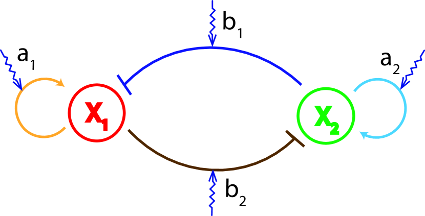
Figure 4: A two-node GRN. Simplified model of the two-node GRN, where the arrowhead and bar-head edges represent activation and inhibition regulation, respectively. The sawtooth lines denote the strength of the tunable edge.

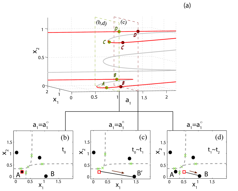
Figure 5: Control of the two-node GRN. (a) Bifurcation diagram with respect to the control parameter $a_{1}$, where the red and gray solid lines denote the stable and unstable steady states, respectively. In the two parallel cross-sections (with dashed line boundaries) for $a_{1}=a_{1}^{0}$ and $a_{1}=a_{1}^{n}$, the yellow and brown dots represent the corresponding stable attractors, respectively. In (b-d), gray dashed lines represent the basin boundaries; black solid circles and green crosses denote attractors and unstable steady states, respectively. (b) For the initial parameter setting, $a_{1}=a_{1}^{0}$, the system is at a low concentration state $\mathbf{A}$, and the target state is $\mathbf{B}$. (c) By changing $a_{1}$ from $a_{1}^{0}$ to $a_{1}^{n}$, attractor $\mathbf{A}$ is destabilized and its original basin is absorbed into that of the intermediate attractor ${\mathbf{B}}^{\prime}$, so the system approaches ${\mathbf{B}}^{\prime}$. (d) When control perturbation upon $a_{1}$ is released, the landscape recovers to that in (b). Once the system has entered the basin of the target state $\mathbf{B}$ during the process in (c), it will evolve spontaneously towards $\mathbf{B}$. Parameters in simulation are $a_{1}^{0}=1.0$, $a_{1}^{n}=1.4$, $t_{0}=0$, $t_{1}=23$, and $t_{2}=40$.

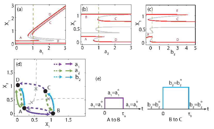
Figure 6: Construction of attractor network for two-node GRN. (a-c) Bifurcation diagrams of the system with respect to the coupling parameters $a_{1}$, $a_{2}$ and $b_{2}$, respectively, where each bifurcation point can be exploited to design control. (d) The corresponding attractor network, in which each directed edge corresponds to an elementary control that is designed to steer the system from the original attractor to the directed one. The solid and dashed edges, respectively, denote the positive and negative changes in the corresponding control parameters. (e) Sequential control signals required to drive the system from attractor $\mathbf{A}$ to attractor $\mathbf{C}$ through the path $\mathbf{A}\rightarrow\mathbf{B}\rightarrow\mathbf{C}$. In simulation, the original parameter values are $a_{1}^{0}=1.0$ and $b_{2}^{0}=0.2$. We set $a_{1}^{n}=1.4$, followed by setting $b_{2}^{n}=4.2$, and the respective durations of the parameter perturbation are $\tau_{a}=23$ and $\tau_{b}=32$.

In a typical experimental setting, four coupling parameters can be adjusted externally through the application of repressive or inductive drugs. To demonstrate attractor network and control implementation, we consider the parameter regime in which the system has four stable steady states (attractors) that correspond to four different cell states during cell development and differentiation. In particular, the dynamical network can be mathematically described as

$$\begin{split}\dot{x_{1}}=a_{1}\cdot\frac{x_{1}^{n}}{s^{n}+x_{1}^{n}}+b_{1}\cdot\frac{s^{n}}{s^{n}+x_{2}^{n}}-k\cdot x_{1},\\ \dot{x_{2}}=a_{2}\cdot\frac{x_{2}^{n}}{s^{n}+x_{2}^{n}}+b_{2}\cdot\frac{s^{n}}{s^{n}+x_{1}^{n}}-k\cdot x_{2},\\ \end{split}$$ (3)

where the dynamical variables $(x_{1},x_{2})$ characterize the protein abundances of the genes products, $k$ denotes the degradation rate of each gene, and the tunable parameters $a_{1}$, $a_{2}$, $b_{1}$, and $b_{2}$ represent the strengths of auto or mutual regulations. In a GRN, the dynamical behaviors of inhibition and activation are captured by the Hill function: $f(x)=x^{n}/(x^{n}+s^{n})$ for activation and $f(x)=s^{n}/(x^{n}+s^{n})$ for inhibition, where the parameter $s$ characterizes half activation (or inhibition) concentration (for $x=s$, the output is $0.5$), and $n$ quantifies the correlation between the input and output concentrations, where a larger value of $n$ corresponds to a stronger inhibition or activation effect. For any specific GRN, the values of both $s$ and $n$ can be determined experimentally. For simplicity, we assume the system to be symmetric in that the inhibition and activation share the same Hill function (i.e., with the same parameters $s$ and $n$). To have four attractors, we set the auto activation strengths, $a_{1}$ and $a_{2}$, to $1.0$, and mutual inhibition strengths, $b_{1}$ and $b_{2}$, to $0.2$. The value of the degradation rate $k$ is set to $1.1$, taking into account the effects of protein degradation and cell volume expansion.

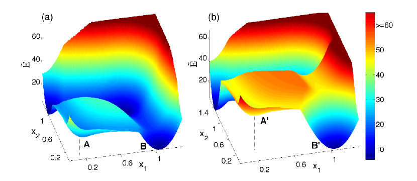
Figure 7: Illustration of pseudo potential landscape. “Pseudo” potential $\tilde{E}$ of the two-node GRN system (a) for $a_{1}=1.0$ ($\Delta_{\mathrm{d}}\approx 0.3549$), $\sigma=0.05$ and (b) for $a_{1}=1.3$ ($\Delta_{\mathrm{d}}\approx 0.0549$), $\sigma=0.05$. Regions of warm and cold colors indicate the states with large and small pseudo energies, respectively.

Figure 5 shows a particular process of controlling the system from an initial state, denoted as ${\mathbf{A}}$, in which both $x_{1}$ and $x_{2}$ have low abundance, to a final state ${\mathbf{B}}$ where $x_{1}$ and $x_{2}$ have high and low abundance, respectively. From the bifurcation diagram [Fig. 5(a)] with respect to the control parameter $a_{1}$, we see that, as $a_{1}$ is increased from $1.0$ to $1.4$, in the lower branch, the initial attractor $\mathbf{A}$ is destabilized through a saddle-node bifurcation. The bifurcation-based control process is shown in Figs. 5(b-d), where panel (b) exhibits the phase space of the system prior to control ($a_{1}=1.0$). When control is activated so that $a_{1}$ is set to $a_{1}=1.4$, the original basin of attraction of attractor ${\mathbf{A}}$ merges into the basin of an intermediate attractor ${\mathbf{B}}^{\prime}$, and the system originally in ${\mathbf{A}}$ starts to migrate towards the intermediate attractor ${\mathbf{B}}^{\prime}$, as indicated by the arrowed trajectory in panel (c). Control perturbation upon $a_{1}$ can be withdrawn once the state of the system enters the region belonging to the original basin of the target attractor $\mathbf{B}$, after which the system spontaneously evolves into $\mathbf{B}$ for $a_{1}=1.0$, as shown in Fig. 5(d).

To obtain a global picture of all possible control outcomes, we construct the attractor network for the two-node GRN system, assuming that three control parameters: $a_{1}$, $a_{2}$ and $b_{2}$, are available for control. The corresponding bifurcation diagrams are shown in Figs. 6(a-c), from which all saddle-node bifurcations can be identified for control design. When all the attractors are connected with directed and weighted edges through the control processes, i.e., when none of the attractor is isolated, we obtain an attractor network, as shown in Fig. 6(d). Specifically, the edge weight can be assigned by taking into account the key characteristics of control such as the critical parameter strength $\mu_{c}$ and the power-law scaling behavior of the required minimum control time $\tau_{m}$ (see Supplementary Table 2). From the attractor network, we can find all possible control paths for any given pair of original and desired states.

From Fig. 6(d), we see that the two-node GRN system is fully controllable since any of the coexisting attractors is reachable by applying proper sequential controls upon the available parameters. The concept of attractor network is appealing because it provides a clear control scenario to drive the system from any initial attractor to any desired attractor. In fact, the attractor network provides a blueprint that can be used to design a proper combination of parameter changes to induce the so-called synergistic or antagonistic effects Yin:2014 . For example, $\mathbf{A}$ is not directly connected with $\mathbf{C}$, neither is $\mathbf{B}$ directly connected to $\mathbf{D}$. However, the system can be steered from $\mathbf{A}$ to $\mathbf{B}$ through perturbation on $a_{1}$, and then from $\mathbf{B}$ to $\mathbf{C}$ through parameter perturbation on $b_{2}$, as shown in Fig. 6(e). Another example to demonstrate the need of multiple parameter perturbation is to control the system from $\mathbf{B}$ to $\mathbf{D}$. A viable control path is $\mathbf{B}\rightarrow\mathbf{C}\rightarrow\mathbf{D}$, which can be realized through perturbation on parameters $(b_{2},a_{1})$. We also see that the two $\mathbf{B}\rightarrow\mathbf{A}\rightarrow\mathbf{D}$ paths can be realized through parameter changes in $(a_{1},a_{2})$ and $(a_{1},b_{2})$, respectively.

When multiple control paths exist from an initial attractor to a final one, a practical issue is to identify an optimal path that is cost effective and robust. The concept of weighted-shortest path can be used to address this issue. Particularly, the weights of edges can be determined from experimental considerations such as the cost, limitation in drug dose, the control duration time, etc.

Potential landscape and beneficial role of noise in nonlinear control.

The role of noise in facilitating control of a nonlinear dynamical network can be understood using the concept of potential landscape WZXW:2011 ; BZA:2011 ; KST:2013 or Waddington landscape Waddington:book in systems biology, which essentially determines the biological paths for cell development and differentiation Huang:2009 ; MML:2009 ; CS:2012 - the landscape metaphor. The potential landscape has been used to manipulate time scales to control stochastic and induced switching in biophysical networks CS:2012 . Intuitively, the power of the concept of the landscape can be understood by resorting to the elementary physical picture of a ball moving in a valley under gravity. The valley thus corresponds to one stable attractor. To the right of the valley there is a hill, or a potential barrier in the language of classical mechanics. The downhill side to the right of the barrier corresponds to a different attractor. Suppose the confinement of ball’s motion within the valley is undesired and one wishes to push the ball over the barrier to the right attractor (desired). If the valley is deep (or the height of the barrier is large), there will be little probability for the ball to move across the top of the barrier towards the desired attractor. In this case, a small amount of noise is unable to enhance the crossover probability. However, if the barrier height is small, a small amount of noise can push the ball over to desired attractor on the right side of the barrier. Thus, the beneficial role of noise is more pronounced for small height of the potential barrier, a behavior that we observe when controlling the T-cell network (Fig. 3). In mechanics, the system can be formulated using a potential function so that, mathematically, the motion of the ball can be described by the Langevin equation, which has been a paradigmatic model to understand nonlinear phenomena such as stochastic resonance BSV:1981 ; BPSV:1983 ; MW:1989 ; MPO:1994 ; GNCM:1997 ; GHJM:1998 . In the past few years, a quantitative approach has been developed to mapping out the potential landscape for gene circuits or gene regulatory networks WXW:2008 ; WXWH:2010 ; WZXW:2011 ; ZXZWW:2012 . In nonlinear dynamical systems, a similar concept exists - quasipotential GT:1984 ; GHT:1991 ; TL:2010 , which plays an important role in understanding phenomena such as noise-induced chaos.

For an attractor network, in the presence of noise each node corresponds to a potential valley of certain depth characterizing the stability of the attractor. For a fixed depth, noise of larger amplitude $\sigma$ leads a larger escaping probability or shorter escaping time. When the amplitude of the control signal is not sufficient to drive the system across the local potential barrier, noise can facilitate control by pushing the system out of the undesired valley (attractor).

The potential landscape for a GRN under Gaussian noise can be constructed from the dynamical equations of the system using the concept of “pseudo” energy KST:2013 (see Methods). For the two-node GRN system [Eq. (3)] subject to stochastic disturbance $N(0,\sigma^{2})$, we can compute the potential landscape for any combination of a system parameter (say $a_{1}$) and the noise amplitude $\sigma$. Figure 7 shows two examples of the landscapes for $a_{1}=1.0$ and $a_{1}=1.3$, where the noise amplitude is $\sigma=0.05$. We see that, for $a_{1}=1.0$, there are four valleys (attractors). For $a_{1}=1.3$, the pseudo energy for $\mathbf{A}$ (the original valley at the lower-left corner) becomes higher, and the path for the transition from $\mathbf{A}$ to $\mathbf{B}$ becomes more pronounced. Further increasing $a_{1}$ towards the critical value (about $1.35$) raises the energy of $\mathbf{A}$ to the level of the potential barrier, effectively eliminating the corresponding valley and the attractor itself.

Attractor network for a three-node GRN.

We also study a three-node GRN system, as shown in Fig. 8(a). Similar to the two-node GRN system, there exist both auto and mutual regulations among the nodes. All the interactions are assumed to be characterized by the same parameters of $s$ and $n$ in the Hill function. The nonlinear dynamical equations of the system are MTELT:2009 ; Shuetal:2013

$$\begin{split}\dot{x_{1}}=a_{1}\cdot\frac{x_{1}^{n}}{s^{n}+x_{1}^{n}}+b_{1}\cdot\frac{s^{n}}{s^{n}+x_{2}^{n}}+c_{1}\cdot\frac{s^{n}}{s^{n}+x_{3}^{n}}-k\cdot x_{1},\\ \dot{x_{2}}=a_{2}\cdot\frac{s^{n}}{s^{n}+x_{1}^{n}}+b_{2}\cdot\frac{x_{2}^{n}}{s^{n}+x_{2}^{n}}+c_{2}\cdot\frac{s^{n}}{s^{n}+x_{3}^{n}}-k\cdot x_{2},\\ \dot{x_{3}}=a_{3}\cdot\frac{s^{n}}{s^{n}+x_{1}^{n}}+b_{3}\cdot\frac{s^{n}}{s^{n}+x_{2}^{n}}+c_{3}\cdot\frac{x_{3}^{n}}{s^{n}+x_{3}^{n}}-k\cdot x_{3},\\ \end{split}$$ (4)

where the state variables ($x_{1}$, $x_{2}$ and $x_{3}$) represent the abundances of the three genes products, the auto-activation parameters $a_{1}$, $b_{2}$, $c_{3}$ and the mutual-inhibition parameters $a_{2}$, $a_{3}$, $b_{1}$, $b_{3}$, $c_{1}$, $c_{2}$ are all experimentally accessible. To be concrete, initially all the auto activation and mutual inhibition parameters are set to be $1.0$ and $0.1$, respectively, and $k$ is the degradation rate that can be conveniently set to unity. The parameters in the Hill function are $n=4$ and $s=0.5$. There are altogether eight attractors in this system, as shown in Fig. 8(b), which are distributed symmetrically in the three-dimensional state space. For example, attractor $\mathbf{H}$ has relatively high values for all three dynamical variables, and attractor $\mathbf{B}$ exhibits the opposite case with low abundances. For attractors $\mathbf{A}$, $\mathbf{C}$ and $\mathbf{F}$, one of the three state variables is high and the other two are low. For attractors $\mathbf{D}$, $\mathbf{E}$ and $\mathbf{G}$, one of the three state variables is low but the other two are high.

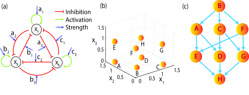
Figure 8: Attractor network and control of a three-node GRN system. (a) Schematic illustration of a three-node GRN system. The arrowhead and bar-head edges represent activation and inhibitory regulations, respectively. The sawtooth lines specify that corresponding edge strength is experimentally adjustable. (b) Coexisting attractors ($\mathbf{A}$ to $\mathbf{H}$) in the phase space. (c) The underlying attractor network, where each node represents an attractor and each weighted directed link indicates that its strength can be experimentally tuned to steer the system from the starting attractor to the pointed attractor.

From numerical simulations, we find that the features of control are essentially the same as those for the two-node GRN system, in terms of characteristics such as the existence of critical control strength and the power-law behavior of the minimum control time (see Table S3 in SI). We construct the attractor network in Fig. 8(c) through combinations of all eight attractors (as nodes) and directed elementary controls (as weighted directed edges). Information in Table S3 can also be used to estimate the respective weights of the edges. From the attractor network, for any given pair of initial and final states, we can identify all the viable control paths. Furthermore, the weighted-shortest path can be calculated once the edge weights are determined.

We note that, typically, the attractor network based on elementary control is not an all-to-all directed network so that certain control paths are absent, e.g., from attractor $\mathbf{H}$ to $\mathbf{B}$. The biological meaning is that, while a stem state can be differentiated into various types of cells through bifurcation, the opposite paths back to the stem state are much more difficult to find.

Discussions

The field of controlling chaos in nonlinear dynamical systems has been active for more than two decades since the seminal work of Ott, Grebogi, and Yorke OGY:1990 . The basic idea was that chaos, while signifying random or irregular behavior, possesses an intrinsically sensitive dependence on initial conditions, which can be exploited for controlling the system using only small perturbations. This feature, in combination with the fact that a chaotic system possesses an infinite set of unstable periodic orbits, each leading to different system performance, implies that a chaotic system can be stabilized about some desired state with optimal performance using small control perturbations. Controlling chaos has since been studied extensively and examples of successful experimental implementation abound in physical, chemical, biological, and engineering systems BGLMM:2000 . The vast literature on controlling chaos, however, has been mostly limited to low-dimensional systems, systems that possess one or a very few unstable directions (i.e., one or a very few positive Lyapunov exponents). Complex networks with nonlinear dynamics are generally high dimensional, rendering inapplicable existing methodologies of chaos control. While mathematical frameworks of controllability of complex networks LSB:2011 ; YZDWL:2013 were developed and extensively studied recently, the deficiency of such rigorous mathematical frameworks is that the nodal dynamical processes must be assumed to be linear. While controllability for nonlinear control can be formulated based on Lie brackets SL:book , it may be difficult to implement the abstract framework for complex networks.

Controlling nonlinear dynamics on complex networks remains to be an outstanding and challenging problem, especially in terms of the two key issues: controllability and actual control. To assess the controllability of nonlinear dynamical networks, drastically different approaches than the linear controllability framework are needed. While there were previous works on specific control methods such as pinning control WC:2002 ; LWC:2004 ; SBGC:2007 and brute-force control that rely on altering the state variables of the underlying system (which in realistic situations can be difficult to implement), we continue to lack a general framework for actual control of complex networks with nonlinear dynamics through realistic, physical means. The main difficulty lies in the extremely diverse nonlinear dynamical behaviors that a network can generate, making it practically impossible to develop a general mathematical framework for control. In particular, the traditional control theoretical tools for linear dynamical systems aim to control the detailed states of all of the variables, which is in fact an overkill for most systems. For nonlinear dynamical networks, a physically meaningful approach may not require detailed control of all state variables. With this relaxation of the control requirement, it may be possible to develop a framework of controllability and devise actual control strategies for nonlinear dynamical networks based on physical/experimental considerations.

A common feature of nonlinear dynamical systems is the emergence of a large number of distinct, coexisting attractors Ott:book ; LT:book . Often the performance and functions of the system are determined by the particular attractor that the system has settled into, associated with which the detailed states of the dynamical variables are not relevant. The key is thus to develop control principles whereby we nudge a complex, nonlinear system from attractor to attractor through small perturbations to a set of physically or experimentally feasible parameters. The main message of this paper is that a controllability framework can be developed for nonlinear dynamical networks based on the control of attractors.

Generally, the reason for control is that the current system is likely to evolve into an undesired state (attractor) or the system is already in such a state, and one wishes to apply perturbations to bring the system out of the undesired state and steer it into a desired state. The first step is then to identify a final state or attractor of the system that leads to the desired performance. The next step is to choose a set of experimentally adjustable parameters and determine whether small perturbations to these parameter can bring the system to the desired attractor. That is, under physically realizable perturbations there should be a control path between the undesired and the desired attractors. The path can be directly from the former to the latter, or there can be intermediate attractors on the path. For example, due to the physical constraint on the control parameters and the ranges in which they can be meaningfully varied, one can drive the system into some intermediate attractors by perturbing one set of parameters, and then from these attractors to the final attractor by using a different set of parameter control. For a complex, nonlinear dynamical network, the number of coexisting attractors can be large. Given a set of system performance indicators, one can classify all the available attractors into three categories: the undesired, desired, and the intermediate attractors. We say a nonlinear network is controllable if there is a control path from any undesired attractor to the desired attractor under finite parameter perturbations. Regarding each attractor as a node and the control paths as directed links or edges, we generate an attractor network whose properties determine the controllability of the original networked dynamical system. For example, the average path length from an undesired to a desired attractor and the “control energy” (or the amount of necessary parameter perturbations) can serve as quantitative measures to characterize the controllability of the original network. We demonstrate our idea of control and construction of attractor networks using realistic networks from systems and synthetic biology. We also find that noise can facilitate control of nonlinear dynamical networks, and we provide a physical theory to understand this counterintuitive phenomenon.

While we emphasize the need to focus on physically meaningful and experimentally accessible parameter perturbations, there can still be a large number of attractor networks depending on the choice of the parameters, making it difficult to formulate a rigorous mathematical framework. We believe that these issues can and will be satisfactorily addressed in the near future, ultimately realizing the grand goal of controlling nonlinear dynamical networks.

Methods

Pseudo potential landscape.

For a dissipative, nonlinear dynamical system subject to noise, we can construct a pseudo potential landscape based on the state probability distribution. Assume that, asymptotically, the system approaches a stationary distribution. For a canonical dynamical system, the potential can be defined as $E({\bf x})=-\log{P({\bf x})}$, where $P({\bf x})$ is the probability density function. For a conservative dynamical system, the direction of system evolution is nothing but the direction of the gradient of the potential function. However, this does not hold for dissipative dynamical systems. The potential function thus does not have the same physical meaning as that for a conservative system, henceforth the term pseudo potential. This approach can be adopted to GRNs.

To obtain the stationary distribution, we use the modified weighted-ensemble algorithm proposed by Kromer et al. KST:2013 , which offers faster convergence than, for example, the traditional random walk method. To be illustrative, we take the two-node GRN system [Eq. (3)] as an example to demonstrate how the pseudo potential landscape can be numerically obtained. The state space of the two-dimensional dynamical system is partitioned into an $M\times M$ lattice with reflective boundaries conditions. Initially the probability $P_{m,n}(t)$ of all gird points are set to be uniform. The simulation time is divided into $T$ steps, where each step has the duration $\tau$. At the beginning of each step $t$, there are $N$ walkers randomly distributed at the grid point $(m,n)$, which carry equal weight $P_{m,n}(t)/N$ and perform random walk under the system dynamics and noise. The locations of these walkers in the grid are recorded at the end of each time step, and the probability at next time step, $P_{m,n}(t+1)$, is the summation of the probabilities carried by all the walkers at time $t$. At time $(t+1)$, $N$ new walkers carrying the updated probability at each grid point perform random walk again on the grid. This procedure repeats until the probability distribution becomes stationary, say $P_{m,n}$, which gives the pseudo potential landscape as $\tilde{E}(m,n)=-\log{P_{m,n}}$. Numerically, the time evolution of all walkers can be simulated using the second-order Heun method for integrating stochastic differential equations. For Fig. 7, the state space is divided into a $500\times 500$ grid. At each grid point there are $N=20$ walkers, each evolving $T=2000$ time steps with $\tau=10^{-4}$.

Author contributions

Devised the research project: YCL, XW, and CG; Performed numerical simulations: LZW and RS; Analyzed the results: LZW, RS, ZGH, YCL, and WXW; Wrote the paper: YCL, LZW, ZGH, and RS.

Additional information

Supplementary Information accompanies this paper.

Competing financial interests

The authors declare no competing financial interests.

References

- (1) Lombardi, A. & Hörnquist, M. Controllability analysis of networks. Phys. Rev. E 75, 056110 (2007).
- (2) Liu, B., Chu, T., Wang, L. & Xie, G. Controllability of a leader-follower dynamic network with switching topology. IEEE Trans. Automat. Contr. 53, 1009–1013 (2008).
- (3) Rahmani, A., Ji, M., Mesbahi, M. & Egerstedt, M. Controllability of multi-agent systems from a graph-theoretic perspective. SIAM J. Contr. Optim. 48, 162–186 (2009).
- (4) Liu, Y.-Y., Slotine, J.-J. & Barabási, A.-L. Controllability of complex networks. Nature (London) 473, 167–173 (2011).
- (5) Wang, W.-X., Ni, X., Lai, Y.-C. & Grebogi, C. Optimizing controllability of complex networks by small structural perturbations. Phys. Rev. E 85, 026115 (2011).
- (6) Yuan, Z.-Z., Zhao, C., Di, Z.-R., Wang, W.-X. & Lai, Y.-C. Exact controllability of complex networks. Nature Commun. 4, 2447 (2013).
- (7) Chen, Y.-Z., Wang, L.-Z., Wang, W.-X. & Lai, Y.-C. The paradox of controlling complex networks: control inputs versus energy requirement. arXiv:1509.03196v1 (2015).
- (8) Nacher, J. C. & Akutsu, T. Dominating scale-free networks with variable scaling exponent: heterogeneous networks are not difficult to control. New J. Phys. 14, 073005 (2012).
- (9) Yan, G., Ren, J., Lai, Y.-C., Lai, C.-H. & Li, B. Controlling complex networks: How much energy is needed? Phys. Rev. Lett. 108, 218703 (2012).
- (10) Nepusz, T. & Vicsek, T. Controlling edge dynamics in complex networks. Nat. Phys. 8, 568–573 (2012).
- (11) Liu, Y.-Y., Slotine, J.-J. & Barabási, A.-L. Observability of complex systems. Proc. Natl. Acad. Sci. (USA) 110, 2460–2465 (2013).
- (12) Menichetti, G., Dall¡¯Asta, L. & Bianconi, G. Network controllability is determined by the density of low in-degree and out-degree nodes. Phys. Rev. Lett. 113, 078701 (2014).
- (13) Ruths, J. & Ruths, D. Control profiles of complex networks. Science 343, 1373–1376 (2014).
- (14) Wuchty, S. Controllability in protein interaction networks. Proc. Natl. Acad. Sci. (USA) 111, 7156–7160 (2014).
- (15) Whalen, A. J., Brennan, S. N., Sauer, T. D. & Schiff, S. J. Observability and controllability of nonlinear networks: The role of symmetry. Phys. Rev. X 5, 011005 (2015).
- (16) Yan, G. et al. Spectrum of controlling and observing complex networks. Nat. Phys. 11, 779–786 (2015).
- (17) Kalman, R. E. Mathematical description of linear dynamical systems. J. Soc. Indus. Appl. Math. Ser. A 1, 152–192 (1963).
- (18) Lin, C.-T. Structural controllability. IEEE Trans. Automat. Contr. 19, 201–208 (1974).
- (19) Luenberger, D. G. Introduction to Dynamical Systems: Theory, Models, and Applications (John Wiley & Sons, Inc, New Jersey, 1999), first edn.
- (20) Wang, X. F. & Chen, G. Pinning control of scale-free dynamical networks. Physica A 310, 521–531 (2002).
- (21) Li, X., Wang, X. F. & Chen, G. Pinning a complex dynamical network to its equilibrium. IEEE Trans. Circ. Syst. I 51, 2074–2087 (2004).
- (22) Sorrentino, F., di Bernardo, M., Garofalo, F. & Chen, G. Controllability of complex networks via pinning. Phys. Rev. E 75, 046103 (2007).
- (23) Chen, Y.-Z., Huang, Z.-G. & Lai, Y.-C. Controlling extreme events on complex networks. Sci. Rep. 4, 6121 (2014).
- (24) Grebogi, C., McDonald, S. W., Ott, E. & Yorke, J. A. Final state sensitivity: an obstruction to predictability. Phys. Lett. A 99, 415–418 (1983).
- (25) McDonald, S. W., Grebogi, C., Ott, E. & Yorke, J. A. Fractal basin boundaries. Physica D 17, 125–153 (1985).
- (26) Feudel, U. & Grebogi, C. Multistability and the control of complexity. Chaos 7, 597–604 (1997).
- (27) Feudel, U. & Grebogi, C. Why are chaotic attractors rare in multistable systems? Phys. Rev. Lett. 91, 134102 (2003).
- (28) Lai, Y.-C. & Tél, T. Transient Chaos - Complex Dynamics on Finite-Time Scales (Springer, New York, 2011), first edn.
- (29) Ni, X., Ying, L., Lai, Y.-C., Do, Y.-H. & Grebogi, C. Complex dynamics in nanosystems. Phys. Rev. E 87, 052911 (2013).
- (30) Alley, R. B. et al. Abrupt climate change. Science 299, 2005–2010 (2003).
- (31) May, R. M. Thresholds and breakpoints in ecosystems with a multiplicity of stable states. Nature 269, 471–477 (1977).
- (32) Schröder, A., Persson, L. & De Roos, A. M. Direct experimental evidence for alternative stable states: a review. Oikos 110, 3–19 (2005).
- (33) Chase, J. M. Experimental evidence for alternative stable equilibria in a benthic pond food web. Ecol. Lett. 6, 733–741 (2003).
- (34) Badzey, R. L. & Mohanty, P. Coherent signal amplification in bistable nanomechanical oscillators by stochastic resonance. Nature 437, 995–998 (2005).
- (35) Wang, J., Zhang, K., Xu, L. & Wang, E. Quantifying the waddington landscape and biological paths for development and differentiation. Proc. Natl. Acad. Sci. (USA) 108, 8257–8262 (2011).
- (36) Huang, S., Guo, Y.-P., May, G. & Enver, T. Bifurcation dynamics in lineage-commitment in bipotent progenitor cells. Developmental Biol. 305, 695–713 (2007).
- (37) Huang, S. Genetic and non-genetic instability in tumor progression: link between the fitness landscape and the epigenetic landscape of cancer cells. Cancer Metastasis Rev. 32, 423–448 (2013).
- (38) Süel, G. M., Garcia-Ojalvo, J., Liberman, L. M. & Elowitz, M. B. An excitable gene regulatory circuit induces transient cellular differentiation. Nature 440, 545–550 (2006).
- (39) Huang, S., Eichler, G., Bar-Yam, Y. & Ingber, D. E. Cell fates as high-dimensional attractor states of a complex gene regulatory network. Phys. Rev. Lett. 94, 128701 (2005).
- (40) Furusawa, C. & Kaneko, K. A dynamical-systems view of stem cell biology. Science 338, 215–217 (2012).
- (41) Li, X., Zhang, K. & Wang, J. Exploring the mechanisms of differentiation, dedifferentiation, reprogramming and transdifferentiation. PloS one 9, e105216 (2014).
- (42) Yao, G., Tan, C., West, M., Nevins, J. & You, L. Origin of bistability underlying mammalian cell cycle entry. Mol. Syst. Biol. 7 (2011).
- (43) Battogtokh, D. & Tyson, J. J. Bifurcation analysis of a model of the budding yeast cell cycle. Chaos 14, 653–661 (2004).
- (44) Kauffman, S., Peterson, C., Samuelsson, B. & Troein, C. Genetic networks with canalyzing boolean rules are always stable. Proc. Natl. Acad. Sci. (USA) 101, 17102–17107 (2004).
- (45) Greil, F. & Drossel, B. Dynamics of critical kauffman networks under asynchronous stochastic update. Phys. Rev. Lett. 95, 048701 (2005).
- (46) Motter, A., Gulbahce, N., Almaas, E. & Barabási, A.-L. Predicting synthetic rescues in metabolic networks. Mol. Sys. Biol. 4 (2008).
- (47) Ma, W., Trusina, A., El-Samad, H., Lim, W. A. & Tang, C. Defining network topologies that can achieve biochemical adaptation. Cell 138, 760–773 (2009).
- (48) Faucon, P. C. et al. Gene networks of fully connected triads with complete auto-activation enable multistability and stepwise stochastic transitions. PloS one 9, e102873 (2014).
- (49) Gardner, T. S., Cantor, C. R. & Collins, J. J. Construction of a genetic toggle switch in escherichia coli. Nature 403, 339–342 (2000).
- (50) Wu, M. et al. Engineering of regulated stochastic cell fate determination. Proc. Natl. Acad. Sci. (USA) 110, 10610–10615 (2013).
- (51) Wu, F., Menn, D. & Wang, X. Quorum-sensing crosstalk-driven synthetic circuits: From unimodality to trimodality. Chem. Biol. 21, 1629–1638 (2014).
- (52) Lai, Y.-C. Controlling complex, nonlinear dynamical networks. Nat. Sci. Rev. 1, 339–341 (2014).
- (53) Feala, J. D. et al. Systems approaches and algorithms for discovery of combinatorial therapies. Wiley Interdiscip. Rev. Syst. Biol. Med. 2, 181–193 (2010).
- (54) Fitzgerald, J. B., Schoeberl, B., Nielsen, U. B. & Sorger, P. K. Systems biology and combination therapy in the quest for clinical efficacy. Nat. Chem. Biol. 2, 458–466 (2006).
- (55) Zhang, R. et al. Network model of survival signaling in large granular lymphocyte leukemia. Proc. Natl. Acad. Sci. (USA) 105, 16308–16313 (2008).
- (56) Saadatpour, A. et al. Dynamical and structural analysis of a t cell survival network identifies novel candidate therapeutic targets for large granular lymphocyte leukemia. PloS Comp. Biol. 7, e1002267 (2011).
- (57) Wittmann, D. M. et al. Transforming boolean models to continuous models: methodology and application to t-cell receptor signaling. BMC Syst. Biol. 3, 98 (2009).
- (58) Krumsiek, J., Pölsterl, S., Wittmann, D. M. & Theis, F. J. Odefy-from discrete to continuous models. BMC Bioinformatcis 11, 233 (2010).
- (59) Cornelius, S. P., Kath, W. L. & Motter, A. E. Realistic control of network dynamics. Nat. Comm. 4, 1942 (2013).
- (60) Benzi, R., Sutera, A. & Vulpiani, A. The mechanism of stochastic resonance. J. Phys. A 14, L453–L457 (1981).
- (61) Benzi, R., Parisi, G., Sutera, A. & Vulpiani, A. A theory of stochastic resonance in climatic-change. J. Appl. Math. 43, 565–578 (1983).
- (62) McNamara, B. & Wiesenfeld, K. Theory of stochastic resonance. Phys. Rev. A 39, 4854–4869 (1989).
- (63) Moss, F., Pierson, D. & O’Gorman, D. Stochastic resonance - tutorial and update. Int. J. Bif. Chaos 4, 1383–1397 (1994).
- (64) Gailey, P. C., Neiman, A., Collins, J. J. & Moss, F. Stochastic resonance in ensembles of nondynamical elements: The role of internal noise. Phys. Rev. Lett. 79, 4701–4704 (1997).
- (65) Gammaitoni, L., Hänggi, P., Jung, P. & Marchesoni, F. Stochastic resonance. Rev. Mod. Phys. 70, 223–287 (1998).
- (66) Sigeti, D. & Horsthemke, W. Pseudo-regular oscillations induced by external noise. J. Stat. Phys. 54, 1217 (1989).
- (67) Pikovsky, A. S. & Kurths, J. Coherence resonance in a noise-driven excitable system. Phys. Rev. Lett. 78, 775–778 (1997).
- (68) Liu, Z. & Lai, Y.-C. Coherence resonance in coupled chaotic oscillators. Phys. Rev. Lett. 86, 4737–4740 (2001).
- (69) Lai, Y.-C. & Liu, Z. Noise-enhanced temporal regularity in coupled chaotic oscillators. Phys. Rev. E 64, 066202 (2001).
- (70) Yin, N. et al. Synergistic and antagonistic drug combinations depend on network topology. PloS one 9, e93960 (2014).
- (71) Bhattacharya, S., Zhang, Q. & Andersen, M. E. A deterministic map of waddington’s epigenetic landscape for cell fate specification. BMC Syst. Biol. 5, 85 (2011).
- (72) Kromer, J. A., Schimansky-Geier, L. & Toral, R. Weighted-ensemble brownian dynamics simulation: Sampling of rare events in nonequilibrium systems. Phys. Rev. E 87, 063311 (2013).
- (73) Waddington, C. H. The Strategy of the Genes (Allen Unwin, London, 1957).
- (74) Huang, S. Reprogramming cell fates: reconciling rarity with robustness. Bioessays 31, 546–560 (2009).
- (75) MacArthur, B. D., Maayan, A. & Lemischka, I. R. Systems biology of stem cell fate and cellular reprogramming. Nat. Rev. Mol. Cell Biol. 10, 672–681 (2009).
- (76) Corson, F. & Siggia, E. D. Geometry, epistasis, and developmental patterning. Proc. Nat. Acad. Sci. (USA) 109, 5568–5575 (2012).
- (77) Wang, J., Xu, L. & Wang, E. K. Potential landscape and flux framework of nonequilibrium networks: Robustness, dissipation, and coherence of biochemical oscillations. Proc. Natl. Acad. Sci. USA 105, 12271–12276 (2008).
- (78) Wang, J., Xu, L., Wang, E. K. & Huang, S. The potential landscape of genetic circuits imposes the arrow of time in stem cell differentiation. Biophys. J. 99, 29–39 (2010).
- (79) Zhang, F., Xu, L., Zhang, K., Wang, E. K. & Wang, J. The potential and flux landscape theory of evolution. J. Chem. Phys. 137, 065102 (2012).
- (80) Garham, R. & Tél, T. Existence of a potential for dissipative dynamical systems. Phys. Rev. Lett. 52, 9–12 (1984).
- (81) Graham, R., Hamm, A. & Tél, T. Nonequilibrium potentials for dynamical systems with fractal attractors and repellers. Phys. Rev. Lett. 66, 3089–3092 (1991).
- (82) Tél, T. & Lai, Y.-C. Quasipotential approach to critical scaling in noise-induced chaos. Phys. Rev. E 81, 056208 (2010).
- (83) Shu, J. et al. Induction of pluripotency in mouse somatic cells with lineage specifiers. Cell 153, 963–975 (2013).
- (84) Ott, E., Grebogi, C. & Yorke, J. A. Controlling chaos. Phys. Rev. Lett. 64, 1196–1199 (1990).
- (85) Boccaletti, S., Grebogi, C., Lai, Y.-C., Mancini, H. & Maza, D. Control of chaos: theory and applications. Phys. Rep. 329, 103–197 (2000).
- (86) Slotine, J.-J. E. & Li, W. Applied Nonlinear Control (Prentice-Hall, New Jersey, 1991).
- (87) Ott, E. Chaos in Dynamical Systems (Cambridge University Press, Cambridge, UK, 2002), second edn.
Acknowledgement
This work was supported by ARO under Grant W911NF-14-1-0504.