Cracking of general relativistic anisotropic polytropes

Abstract

We discuss the effect that small fluctuations of local anisotropy of pressure, and of energy density, may have on the occurrence of cracking in spherical compact objects, satisfying a polytropic equation of state. Two different kinds of polytropes are considered. For both, it is shown that departures from equilibrium may lead to the appearance of cracking, for a wide range of values of the parameters defining the polytrope. Prospective applications of the obtained results, to some astrophysical scenarios, are pointed out.

I Introduction

In recent papers the general formalism to study polytropes for anisotropic matter has been presented, both in the Newtonian 1p and the general relativistic regimes 2p ; 3p . The motivations to undertake such a task were, on the one hand, the fact that the polytropic equations of state allow to deal with a variety of fundamental astrophysical problems (see Refs. cha ; sch ; 2 ; 3 ; 7' ; 9 ; 8 ; 10 ; 4a ; 4b ; 4c ; 5 ; 6 ; 7 ; 11 ; 12 ; 13 ; pol1n and references therein).

On the other hand, the local anisotropy of pressure may be caused by a large variety of physical phenomena of the kind we expect to find in compact objects (see Refs. 14 ; 04 ; hmo02 ; hod08 ; hsw08 ; p1 ; p2 ; anis1 ; anis2 ; anis3 ; anis4bis , and references therein for an extensive discussion on this point).

Among all possible sources of anisotropy (see 14 for a comprehensive discussion on this point), let us mention two which might be particularly related to our primary interest. The first one is the intense magnetic field observed in compact objects such as white dwarfs, neutron stars, or magnetized strange quark stars (see, for example, Refs. 15 ; 16 ; 17 ; 18 ; 19 and references therein). Indeed, it is a well-established fact that a magnetic field acting on a Fermi gas produces pressure anisotropy (see Refs. 23 ; 24 ; 25 ; 26 and references therein). In some way, the magnetic field can be addressed as a fluid anisotropy (however, it should be observed that for the thermodynamic pressure of degenerate particles under the conditions of Landau quantization, it remains isotropic bla ).

Another source of anisotropy expected to be present in neutron stars and, in general, in highly dense matter, is the viscosity (see Anderson ; sad ; alford ; blaschke ; drago ; jones ; vandalen ; Dong and references therein). At this point it is worth noticing that we are not concerned by how small the resulting anisotropy produced by the viscosity might be, since as we shall see below, the occurrence of crackings may happen even for slight deviations from isotropy.

An alternative approach to anisotropy comes from kinetic theory using the spherically symmetric Einstein-Vlasov equations, which admits a very rich class of static solutions, none of them isotropic (Ref. ref1 ; andreasson ; ref2 and references therein). The advantages or disadvantages of either approach being related to the specific problem under consideration.

The theory of polytropes is based on the polytropic equation of state, which in the Newtonian case reads

$$P=K\rho_{0}^{\gamma}=K\rho_{0}^{1+1/n},$$ (1)

where $P$ and $\rho_{0}$ denote the isotropic pressure and the mass (baryonic) density, respectively. Constants $K$, $\gamma$, and $n$ are usually called the polytropic constant, polytropic exponent, and polytropic index, respectively.

In the general relativistic, anisotropic, case, two possible extensions of the above equation of state are possible, namely:

1. $$P_{r}=K\rho_{0}^{\gamma}=K\rho_{0}^{1+1/n},$$ (2)

2. $$P_{r}=K\rho^{\gamma}=K\rho^{1+1/n},$$ (3)

where $P_{r}$ and $\rho$ denote the radial pressure (see below), and the energy density respectively.

As it should be expected, the assumption of either (2) or (3) is not enough to integrate completely the field equations, since the appearance of two principal stresses (instead of one as in the isotropic case) leads to a system of two equations for three unknown functions.

Thus in order to integrate the obtained system of equations we need to provide further information about the anisotropy, inherent to the problem under consideration. For doing that, in 2p a particular ansatz anis4 has been assumed, which allows for specific modelling. This method links the obtained models continually with the isotropic case, thereby allowing us to bring out the influence of anisotropy on the structure of the object, even for very small anistropies. Here we shall adopt the above mentioned ansatz. However it should be stressed that our models are presented with the sole purpose of illustrating the occurrence of crackings; the natural way to obtain models, consists of providing the specific information about the kind of anisotropy present in each specific problem.

The concept of cracking was introduced to describe the behavior of a fluid distribution just after its departure from equilibrium, when total nonvanishing radial forces of different signs appear within the system cn .

Thus, if we take a snapshot of the system, just after leaving equilibrium (on a time scale smaller than the hydrostatic time scale), we say that there is a cracking whenever this radial force is directed inwards in the inner part of the sphere and reverses its sign beyond some value of the radial coordinate. In the opposite case, when the force is directed outwards in the inner part and changes sign in the outer part, we say that there is an overturning. Further developments on this issue may be found in cnbis ; cn1 ; cn2 ; cn4 ; cn5 ; cn7bis ; cn7bbis ; mardam . As should be clear at this point, the concept of cracking is closely related to the problem of structure formation cn3 ; cn6 ; cn7 .

In the example examined in cn it appears that cracking occurs only in the locally anisotropic case whereas in the perfect fluid case, once out of equilibrium, the configuration tends either to collapse or to expand as a whole. Furthermore it has been shown in cn1 , that for a wide range of models, cracking appears only if, in the process of perturbation leading to departure from equilibrium, the local anisotropy is perturbed. This result suggests that fluctuations of local anisotropy may be the crucial factor in the occurrence of cracking. Thus, in the case of an initially locally isotropic configuration, the appearance of cracking shows that even small deviations from local isotropy may lead to drastic changes in the evolution of the system as compared with the purely locally isotropic case cn1 .

It is the purpose of this work to study in some detail the conditions under which, cracking appears in anisotropic polytropes. We shall consider the two possible cases of anisotropic polytropes mentioned above, and our models are the same as those considered in 2p .

At this point, we have to make some comments about the perturbative scheme, leading to departures from equilibrium. For the cracking to occur, it is imperative that the perturbations introduced into the system take it out of equilibrium. In other words we shall consider, exclusively, perturbations under which the system is dynamically unstable. One way to assure this, is to assume that the value of the ratio of specific heats of the fluid is not equal to the critical value required for marginal (neutral) dynamical stability. So, under perturbations, the configuration either collapses or expands. Another completely equivalent way to achieve this instability consists in assuming that, under perturbations of density and local anisotropy, the radial pressure of the system maintains the same radial dependence it had in equilibrium. It is obvious that in this case the hydrostatic equation will no longer be satisfied.

It should be clear that assuming this lack of response of the fluid, i.e. the inability to adapt its radial pressure to the perturbed situation, is equivalent to assuming that the pressure-density relation (the ratio of specific heats) never reaches the value required for neutral equilibrium.

In this work, we shall consider two possible ways to perturb the energy density and the local anisotropy, namely:

• We shall perturb the parameter $K$ and the parameter describing the anisotropy.

  or

• We shall perturb the parameter $n$ and the parameter describing the anisotropy.

As we shall see, cracking occurs for a wide range of values of the parameters.

II Relevant Equations and Conventions

II.1 The field equations

Even though polytropes are static configurations, we have to keep in mind that the appearance of cracking occurs when the system is taken out of equilibrium. Accordingly, we shall consider spherically symmetric distributions of collapsing fluid, which we assume to be locally anisotropic, bounded by a spherical surface $\Sigma$. The static limit is trivially recovered from the equations below.

The line element is given in Schwarzschild-like coordinates by

$$ds^{2}=e^{\nu}dt^{2}-e^{\lambda}dr^{2}-r^{2}\left(d\theta^{2}+\sin^{2}\theta d\phi^{2}\right),$$ (4)

where $\nu(t,r)$ and $\lambda(t,r)$ are functions of their arguments. We number the coordinates: $x^{0}=t;\,x^{1}=r;\,x^{2}=\theta;\,x^{3}=\phi$.

which in our case read cn :

$$-8\pi T^{0}_{0}=-\frac{1}{r^{2}}+e^{-\lambda}\left(\frac{1}{r^{2}}-\frac{\lambda^{\prime}}{r}\right),$$ (5)

$$-8\pi T^{1}_{1}=-\frac{1}{r^{2}}+e^{-\lambda}\left(\frac{1}{r^{2}}+\frac{\nu^{\prime}}{r}\right),$$ (6)

$$-8\pi T^{2}_{2} = -8\pi T^{3}_{3}=-\frac{e^{-\nu}}{4}\left[2\ddot{\lambda}+\dot{\lambda}(\dot{\lambda}-\dot{\nu})\right]$$ (7)

$$+ \frac{e^{-\lambda}}{4}\left[2\nu^{\prime\prime}+\nu^{\prime 2}-\lambda^{\prime}\nu^{\prime}+2\frac{\nu^{\prime}-\lambda^{\prime}}{r}\right],$$

$$-8\pi T_{01}=-\frac{\dot{\lambda}}{r},$$ (8)

where dots and primes stand for partial differentiation with respect to $t$ and $r$ respectively.

In order to give physical significance to the $T^{\mu}_{\nu}$ components we apply the Bondi approach Bo .

Thus, following Bondi, let us introduce purely locally Minkowski coordinates ($\tau,x,y,z$)

$$d\tau=e^{\nu/2}dt,\quad\,dx=e^{\lambda/2}dr,\quad\,dy=rd\theta,\quad\,dz=r\sin\theta d\phi.$$

Then, denoting the Minkowski components of the energy tensor by a bar, we have

$$\bar{T}^{0}_{0}=T^{0}_{0},\,\qquad\,\bar{T}^{1}_{1}=T^{1}_{1},\,\qquad\,\bar{T}^{2}_{2}=T^{2}_{2},\,$$

$$\bar{T}^{3}_{3}=T^{3}_{3},\,\qquad\,\bar{T}_{01}=e^{-(\nu+\lambda)/2}T_{01}.$$ (9)

Next, we suppose that when viewed by an observer moving relative to these coordinates with proper velocity $\omega$ in the radial direction, the physical content of space consists of an anisotropic fluid of energy density $\rho$, radial pressure $P_{r}$ and tangential pressure $P_{\bot}$. Thus, when viewed by this moving observer the covariant tensor in Minkowski coordinates is

$$\left(\begin{array}[]{cccc}\rho&0&0&0\\ 0&P_{r}&0&0\\ 0&0&P_{\bot}&0\\ 0&0&0&P_{\bot}\end{array}\right).$$

Then a Lorentz transformation readily shows that

$$T^{0}_{0}=\bar{T}^{0}_{0}=\frac{\rho+P_{r}\omega^{2}}{1-\omega^{2}},$$ (10)

$$T^{1}_{1}=\bar{T}^{1}_{1}=-\frac{P_{r}+\rho\omega^{2}}{1-\omega^{2}},$$ (11)

$$T^{2}_{2}=T^{3}_{3}=\bar{T}^{2}_{2}=\bar{T}^{3}_{3}=-P_{\bot},$$ (12)

$$T_{01}=e^{(\nu+\lambda)/2}\bar{T}_{01}=-\frac{(\rho+P_{r})\omega e^{(\nu+\lambda)/2}}{1-\omega^{2}}.$$ (13)

Note that the coordinate velocity in the ($t,r,\theta,\phi$) system, $dr/dt$, is related to $\omega$ by

$$\omega=\frac{dr}{dt}\,e^{(\lambda-\nu)/2}.$$ (14)

Feeding back (10–13) into (5–8), we get the field equations in the form

$$\frac{\rho+P_{r}\omega^{2}}{1-\omega^{2}}=-\frac{1}{r^{2}}+e^{-\lambda}\left(\frac{1}{r^{2}}-\frac{\lambda^{\prime}}{r}\right),$$ (15)

$$\frac{P_{r}+\rho\omega^{2}}{1-\omega^{2}}=\frac{1}{r^{2}}-e^{-\lambda}\left(\frac{1}{r^{2}}+\frac{\nu^{\prime}}{r}\right),$$ (16)

$$P_{\bot}= \frac{e^{-\nu}}{4}\left[2\ddot{\lambda}+\dot{\lambda}(\dot{\lambda}-\dot{\nu})\right]$$ (17)

$$- \frac{e^{-\lambda}}{4}\left[2\nu^{\prime\prime}+\nu^{\prime 2}-\lambda^{\prime}\nu^{\prime}+2\frac{\nu^{\prime}-\lambda^{\prime}}{r}\right],$$

$$\frac{(\rho+P_{r})\omega e^{(\nu+\lambda)/2}}{1-\omega^{2}}=\frac{\dot{\lambda}}{r}.$$ (18)

At the outside of the fluid distribution, the spacetime is that of Schwarzschild, given by

$$ds^{2}=\left(1-\frac{2M}{{r}}\right)dt^{2}-\frac{dr^{2}}{\left(1-\frac{2M}{{r}}\right)}-r^{2}\left(d\theta^{2}+\sin^{2}\theta d\phi^{2}\right).$$ (19)

In order to match smoothly the two metrics above on the boundary surface $r=r_{\Sigma}(t)$, we require the continuity of the first and the second fundamental forms, across that surface.

These last conditions imply

$$e^{\nu_{\Sigma}}=1-\frac{2M}{r_{\Sigma}},$$ (20)

$$e^{-\lambda_{\Sigma}}=1-\frac{2M}{r_{\Sigma}},$$ (21)

$$[P_{r}]_{\Sigma}=0,$$ (22)

where, from now on, subscript $\Sigma$ indicates that the quantity is evaluated at the boundary surface $\Sigma$. Eqs. (20), (21) and (22) are the necessary and sufficient conditions for a smooth matching of the two metrics (4) and (19) on $\Sigma$.

The energy momentum tensor may be written as:

$$T_{\mu\nu}=\left(\rho+P_{\bot}\right)u_{\mu}u_{\nu}-P_{\bot}g_{\mu\nu}+\left(P_{r}-P_{\bot}\right)s_{\mu}s_{\nu},$$ (23)

where $u^{\mu}$ denotes the four velocity of the fluid and $s^{\mu}$ is a unit spacelike vector, radially directed. These vectors are defined by

$$u^{\mu}=\left[\frac{e^{-\nu/2}}{\left(1-\omega^{2}\right)^{1/2}},\frac{\omega e^{-\lambda/2}}{\left(1-\omega^{2}\right)^{1/2}},0,0\right],$$ (24)

$$s^{\mu}=\left[\frac{\omega\,e^{-\nu/2}}{\left(1-\omega^{2}\right)^{1/2}},\,\frac{e^{-\lambda/2}}{\left(1-\omega^{2}\right)^{1/2}},\,0,\,0\right].$$ (25)

Next, it will be useful to calculate the radial component of the “conservation law”

$$T^{\mu}_{\nu;\mu}=0,$$ (26)

which in the static case becomes

$$R\equiv P^{\prime}_{r}+\frac{\nu^{\prime}}{2}\left(\rho+P_{r}\right)-\frac{2\left(P_{\bot}-P_{r}\right)}{r}=0,$$ (27)

representing the generalization of the Tolman-Oppenheimer-Volkof equation for anisotropic fluids 14 . Alternatively, using

$$\frac{\;\nu^{\prime}}{2}=\frac{m+4\pi P_{r}r^{3}}{r\left(r-2m\right)},$$ (28)

which follows from (15) and (16) in the static case, we may write

$$P^{\prime}_{r}=-\frac{(m+4\pi P_{r}r^{3})}{r\left(r-2m\right)}\left(\rho+P_{r}\right)+\frac{2\left(P_{\bot}-P_{r}\right)}{r},$$ (29)

where the mass function $m(r)$, as usually, is defined by

$$e^{-\lambda}=1-2m/r,\qquad m(r)=4\pi\int^{r}_{0}{\rho r^{2}dr}.$$ (30)

Polytropes are static fluid configurations, which satisfy either of the equation (2) or (3). The full set of equations describing the structure of these self-gravitating objects, in both cases, were derived and discussed in 2p .

All the models have to satisfy physical requirements such as:

$$\rho>0,\qquad\frac{P_{r}}{\rho}\leq 1,\qquad\frac{P_{\perp}}{\rho}\leq 1.$$ (31)

In what follows, we shall very briefly review the main equations corresponding to each case.

II.2 Case I

Assuming Eq. (2), let us introduce the following variables

$$\alpha=P_{rc}/\rho_{c},\quad r=\xi/A,\quad A^{2}=4\pi\rho_{c}/\alpha(n+1),$$ (32)

$$\Psi_{0}^{n}=\rho_{0}/\rho_{0c},\quad v(\xi)=m(r)A^{3}/(4\pi\rho_{c}),$$ (33)

where subscript $c$ indicates that the quantity is evaluated at the center. At the boundary surface $r=r_{\Sigma}$ ($\xi=\xi_{\Sigma}$) we have $\Psi_{0}(\xi_{\Sigma})=0$.

Then, the generalized Tolman-Opphenheimer-Volkoff equation becomes

$$\xi^{2}\frac{d\Psi_{0}}{d\xi}\left[\frac{1-2(n+1)\alpha v/\xi}{(1-n\alpha)+(n+1)\alpha\Psi_{0}}\right]+v+\alpha\xi^{3}\Psi_{0}^{n+1}-\frac{2\Delta\Psi_{0}^{-n}\xi}{P_{rc}(n+1)}\left[\frac{1-2\alpha(n+1)v/\xi}{(1-n\alpha)+(n+1)\alpha\Psi_{0}}\right]=0,$$ (34)

where $\Delta=P_{\bot}-P_{r}$.

On the other hand we obtain from the mass function definition (30) and Eq. (15),

$$m^{\prime}=4\pi r^{2}\rho,$$ (35)

or

$$\frac{dv}{d\xi}=\xi^{2}\Psi_{0}^{n}(1-n\alpha+n\alpha\Psi_{0}).$$ (36)

In this case, conditions (31) read

$$n\alpha<1,\qquad\frac{\alpha\Psi_{0}}{1-n\alpha+n\alpha\Psi_{0}}\leq 1,$$

$$\frac{3v/\xi^{3}+\alpha\Psi_{0}^{n+1}}{\Psi_{0}^{n}(1-n\alpha+n\alpha\Psi_{o})}-1\leq 1.$$ (37)

II.3 Case II

In this case the assumed equation of state is (3), then, introducing

$$\Psi^{n}=\rho/\rho_{c},$$ (38)

the generalized Tolman-Opphenheimer-Volkoff equation becomes

$$\xi^{2}\frac{d\Psi}{d\xi}\left[\frac{1-2(n+1)\alpha v/\xi}{1+\alpha\Psi}\right]+v+\alpha\xi^{3}\Psi^{n+1}-\frac{2\Delta\Psi^{-n}\xi}{P_{rc}(n+1)}\left[\frac{1-2\alpha(n+1)v/\xi}{1+\alpha\Psi}\right]=0,$$ (39)

and from Eq. (35)

$$\frac{dv}{d\xi}=\xi^{2}\Psi^{n}.$$ (40)

In this case, conditions (31) read:

$$\rho>0,\qquad\alpha\Psi\leq 1,\qquad\frac{3v}{\xi^{3}\Psi^{n}}+\alpha\Psi-1\leq 1.$$ (41)

Equations (34), (36) or (39), (40), form a system of two first order ordinary differential equations for the three unknown functions: $\Psi(\Psi_{0}),v,\Delta$, depending on a duplet of parameters $n,\alpha$. Thus, it is obvious that in order to proceed further with the modeling of a compact object, we need to provide additional information. Such information, of course, depends on the specific physical problem under consideration. Here, we shall further assume the equation of state used in anis4 ; 2p .

III Perturbing the anisotropic polytrope

Let us now consider an anisotropic polytrope satisfying the equation of hydrostatic equilibrium (27). Furthermore, our distribution satisfies the equation of state proposed in anis4 , i.e.

$$\Delta=C(\rho+P_{r})\left[\frac{m+4\pi P_{r}r^{3}}{r(r-2m)}\right]r,$$ (42)

where $C$ is a constant, producing

$$R=\frac{dP_{r}}{dr}+h\left[\frac{m+4\pi r^{3}P_{r}}{r(r-2m)}\right](\rho+P_{r})=0,$$ (43)

with

$$h\equiv 1-2C.$$ (44)

In order to observe an eventual cracking, we have to take the system out of equilibrium. For doing so we shall perturb the energy density and the anisotropy, through the parameters $K$ and $h$, or, alternatively, through the parameters $n$ and $h$. Below we describe this procedure for the cases I and II.

III.1 Perturbation in the case I

In this case the following equations apply

$$P_{r}=K\rho^{1+1/n}_{0}\quad\mbox{and}\quad\rho=\rho_{0}+nK\rho_{0}^{1+1/n}.$$ (45)

Then, perturbing the energy density and the local anisotropy via $K$ and $h$,

$$K\longrightarrow\tilde{K} = K+\delta K,$$ (46)

$$h\longrightarrow\tilde{h} = h+\delta h,$$ (47)

it follows that

$$\tilde{P}_{r}=\tilde{K}\rho_{0}^{1+1/n}=\beta P_{r},$$ (48)

$$\tilde{\rho}=\rho_{0}+n\tilde{K}\rho_{0}^{1+1/n}=\rho_{0}+n\beta P_{r},$$ (49)

with

$$\beta=\frac{\tilde{K}}{K},$$ (50)

where the tilde denotes the perturbed quantity.

Introducing the dimensionless variable

$$\hat{\tilde{R}}=\frac{A}{4\pi\rho_{c}^{2}}\tilde{R},$$ (51)

we obtain from (45)-(50)

$$\hat{\tilde{R}}=\beta\Psi_{0}^{n}\frac{d\Psi_{0}}{d\xi}+\frac{\tilde{h}\Psi^{n}_{0}}{\xi^{2}}\left[(1-n\alpha)+\alpha\beta(n+1)\Psi_{0}\right]\left[\frac{\tilde{\upsilon}+\xi^{3}\beta\alpha\Psi_{0}^{n+1}}{1-2\alpha(n+1)\tilde{\upsilon}/\xi}\right].$$ (52)

From the above, it follows that up to first order, we may write

$$\delta\hat{R}=\hat{\tilde{R}}(\xi,1+\delta\beta,h+\delta h,\upsilon+\delta\upsilon)=\hat{R}(\xi,1,h,\upsilon)+\left.\left(\frac{\partial\hat{\tilde{R}}}{\partial\beta}\right)\right|_{\begin{array}[]{c}\beta=1\\ \tilde{h}=h\\ \tilde{\upsilon}=\upsilon\end{array}}.\delta\beta+\left.\left(\frac{\partial\hat{\tilde{R}}}{\partial\tilde{\upsilon}}\right)\right|_{\begin{array}[]{c}\beta=1\\ \tilde{h}=h\\ \tilde{\upsilon}=\upsilon\end{array}}.\delta\upsilon+\left.\left(\frac{\partial\hat{\tilde{R}}}{\partial\tilde{h}}\right)\right|_{\begin{array}[]{c}\beta=1\\ \tilde{h}=h\\ \tilde{\upsilon}=\upsilon\end{array}}.\delta h.$$ (53)

where

$$\hat{\tilde{R}}(\xi,1,h,\upsilon)=0,$$ (54)

as it must be, since the system is at equilibrium in the unperturbed state.

Thus, we may write

$$\delta\hat{R}=\left.\left(\frac{\partial\hat{\tilde{R}}}{\partial\beta}\right)\right|_{\begin{array}[]{c}\beta=1\\ \tilde{h}=h\\ \tilde{\upsilon}=\upsilon\end{array}}.\delta\beta+\left.\left(\frac{\partial\hat{\tilde{R}}}{\partial\tilde{\upsilon}}\right)\right|_{\begin{array}[]{c}\beta=1\\ \tilde{h}=h\\ \tilde{\upsilon}=\upsilon\end{array}}.\delta\upsilon+\left.\left(\frac{\partial\hat{\tilde{R}}}{\partial\tilde{h}}\right)\right|_{\begin{array}[]{c}\beta=1\\ \tilde{h}=h\\ \tilde{\upsilon}=\upsilon\end{array}}.\delta h.$$ (64)

Then, using (52) we obtain

$$\left.\left(\frac{\partial\hat{\tilde{R}}}{\partial\beta}\right)\right|_{\begin{array}[]{c}\beta=1\\ \tilde{h}=h\\ \tilde{\upsilon}=\upsilon\end{array}} = \Psi_{0}^{n}\frac{d\Psi_{0}}{d\xi}+h\frac{\Psi_{0}^{n+1}}{\xi^{2}}\alpha\left[\frac{(n+1)(\upsilon+2\xi^{3}\alpha\Psi_{0}^{n+1})+\xi^{3}\Psi_{0}^{n}(1-n\alpha)}{1-2\alpha(n+1)\upsilon/\xi}\right],$$ (68)

$$\left.\left(\frac{\partial\hat{\tilde{R}}}{\partial\tilde{\upsilon}}\right)\right|_{\begin{array}[]{c}\beta=1\\ \tilde{h}=h\\ \tilde{\upsilon}=\upsilon\end{array}} = h\frac{\Psi_{0}^{n}}{\xi^{2}}\left[\frac{(1-n\alpha)+\alpha(n+1)\Psi_{0}}{(1-2\alpha(n+1)\upsilon/\xi)^{2}}\right][1+2\alpha^{2}(n+1)\xi^{2}\Psi_{0}^{n+1}],$$ (72)

$$\left.\left(\frac{\partial\hat{\tilde{R}}}{\partial\tilde{h}}\right)\right|_{\begin{array}[]{c}\beta=1\\ \tilde{h}=h\\ \tilde{\upsilon}=\upsilon\end{array}} = \frac{\Psi_{0}^{n}}{\xi^{2}}\left[(1-n\alpha)+\alpha(n+1)\Psi_{0}\right]\left[\frac{\upsilon+\xi^{3}\alpha\Psi_{0}^{n+1}}{1-2\alpha(n+1)\upsilon/\xi}\right].$$ (76)

Furthermore, we have

$$\tilde{\upsilon}=\frac{1}{\rho_{c}}\int_{0}^{\xi}\bar{\xi}^{2}\Psi^{n}_{0}(\rho_{0c}+n\beta P_{rc}\Psi_{0})d\bar{\xi},$$ (77)

and

$$\delta\upsilon=\left.\left(\frac{\partial\tilde{\upsilon}}{\partial\beta}\right)\right|_{\beta=1}.\delta\beta,$$ (78)

producing

$$\delta\upsilon=n\alpha\left(\int_{0}^{\xi}\bar{\xi}^{2}\Psi_{0}^{n+1}d\bar{\xi}\right)\delta\beta=n\alpha F(\xi)\delta\beta,$$ (79)

with

$$F(\xi)\equiv\int_{0}^{\xi}\bar{\xi}^{2}\Psi_{0}^{n+1}d\bar{\xi}.$$ (80)

From the equations above, we may write

$$\delta\hat{R}=\Psi_{0}^{n}\left\{\frac{d\Psi_{0}}{d\xi}+\frac{h\alpha}{\xi^{2}(1-2\alpha(n+1)\upsilon/\xi)}\left[(n+1)(\upsilon+2\xi^{3}\alpha\Psi_{0}^{n+1})\Psi_{0}+\xi^{3}\Psi_{0}^{n+1}(1-n\alpha)\right.\right.$$

$$+\left.\left.\left[\frac{(1-n\alpha)+\alpha(n+1)\Psi_{0}}{1-2\alpha(n+1)\upsilon/\xi}\right]\left[1+2\alpha^{2}(n+1)\xi^{2}\Psi_{0}^{n+1}\right]nF(\xi)\right]\right\}\delta\beta$$

$$+\frac{\Psi_{0}^{n}}{\xi^{2}}\left[(1-n\alpha)+\alpha(n+1)\Psi_{0}\right]\left[\frac{\upsilon+\xi^{3}\alpha\Psi_{0}^{n+1}}{1-2\alpha(n+1)\upsilon/\xi}\right]\delta h.$$ (81)

It would be more convenient to use the variable $x$, defined by

$$x=\frac{\xi}{\bar{A}},\quad\bar{A}=r_{\Sigma}A=\xi_{\Sigma},$$ (82)

in terms of which, (81) becomes

$$\delta\hat{{R}} = \frac{\Psi_{0}^{n}}{\bar{A}}\left\{\frac{d\Psi_{0}}{dx}+\frac{h\alpha}{x(\bar{A}x-2\alpha(n+1)\upsilon)}\left[(n+1)(\upsilon+2\bar{A}^{3}x^{3}\alpha\Psi_{0}^{n+1})\Psi_{0}\bar{A}^{3}x^{3}\Psi_{0}^{n+1}(1-n\alpha)\right.\right.$$ (83)

$$+ \left.\left.\bar{A}x\left[\frac{1-n\alpha+\alpha(n+1)\Psi_{0}}{\bar{A}x-2\alpha(n+1)\upsilon}\right](1+2\alpha^{2}(n+1)\bar{A}^{2}x^{2}\Psi_{0}^{n+1})nF_{1}\right]\right\}\delta\beta$$

$$+ \frac{\Psi_{0}^{n}}{\bar{A}x}\left(1-n\alpha+\alpha(n+1)\Psi_{0}\right)\left[\frac{\upsilon+\bar{A}^{3}x^{3}\Psi_{0}^{n+1}}{\bar{A}x-2\alpha(n+1)\upsilon}\right]\delta h.$$

Now, for the cracking to occur, once the system has been perturbed, there must be a change of sign in $\delta\hat{R}$. More specifically, it should be positive in the inner regions, and negative at the outer ones (in the inverse case an overturning is produced). This last condition implies that $\delta\hat{R}=0$ for some value of $\xi$ in the interval $[0,\xi_{\Sigma}]$, implying in turn:

$$\delta h=-\Gamma\delta\beta,$$ (84)

where

$$\Gamma=\left.\left[\frac{\frac{\partial\tilde{R}}{\partial\beta}+\frac{\partial\tilde{R}}{\partial\tilde{\upsilon}}F(\xi)}{\frac{\partial\tilde{R}}{\partial\tilde{h}}}\right]\right|_{\begin{array}[]{c}\beta=1\\ \tilde{\upsilon}=\upsilon\\ \tilde{h}=h\end{array}}.$$ (88)

Another perturbative scheme may be proposed, based on the perturbation of the energy density and the anisotropy through the parameters $n$ and $h$. In this case, following the same line of arguments as in the previous scheme, we have

$$P_{r} = k\rho_{0}^{1+1/n}=k\rho_{0c}^{1+1/n}\Psi_{0}^{n+1}$$ (89)

$$\rho = \rho_{0}+nP_{r}=\rho_{0c}\Psi_{0}^{n}+nk\rho_{0c}^{1+1/n}\Psi_{0}^{n+1}$$ (90)

$$n\longrightarrow\tilde{n} = n+\delta n$$ (91)

$$h\longrightarrow\tilde{h} = h+\delta h.$$ (92)

Then, assuming that the radial pressure remains unchanged under perturbation (what ensures the departure from equilibrium)

$$\tilde{P_{r}}=P_{r},$$ (93)

we have

$$\tilde{P_{r}}=P_{r}=k\rho_{0c}^{1+1/n}\Psi^{n+1},$$ (94)

$$\tilde{\rho}=\rho_{0c}\Psi^{\tilde{n}}+\tilde{n}P_{r}.$$ (95)

Then, replacing into the hydrostatic equlibrium equation, it follows that

$$\hat{\tilde{R}}=\Psi_{0}^{n}\frac{d\Psi_{0}}{d\xi}+\frac{\tilde{h}}{\xi^{2}}[(1-n\alpha)\Psi_{0}^{\tilde{n}}+(\tilde{n}+1)\alpha\Psi_{0}^{n+1}]\left[\frac{\tilde{\upsilon}+\xi^{3}\alpha\Psi_{0}^{n+1}}{(1-2\alpha(n+1)\tilde{\upsilon}/\xi)}\right].$$ (96)

Proceeding exactly as in the previous scheme, we obtain

$$\delta\hat{{R}} = \frac{h\Psi_{0}^{n}}{\xi^{2}\left(1-2\alpha(n+1)\upsilon/\xi\right)}\left[(\upsilon+\xi^{3}\alpha\Psi_{0}^{n+1})((1-n\alpha)\ln(\Psi_{0})+\alpha\Psi_{0})+\left[\frac{1-n\alpha+(1+n)\alpha\Psi_{0}}{1-2\alpha(n+1)\upsilon/\xi}\right](1+2\alpha^{2}\xi^{2}(n+1)\Psi_{0}^{n+1})F_{1n}\right]\delta n$$ (97)

$$+ \frac{\Psi_{0}^{n}}{\xi^{2}}[1-n\alpha+(n+1)\alpha\Psi_{0}]\left[\frac{\upsilon+\xi^{3}\alpha\Psi_{0}^{n+1}}{1-2\alpha(n+1)\upsilon/\xi}\right]\delta h,$$

or,

$$\delta\hat{{R}} = \frac{h\Psi_{0}^{n}}{\bar{A}x(\tilde{A}x-2\alpha(n+1)\upsilon)}\left[(\upsilon+\bar{A}^{3}x^{3}\alpha\Psi_{0}^{n+1})((1-n\alpha)\ln(\Psi_{0})+\alpha\Psi_{0})\right.$$ (98)

$$+ \left.\bar{A}x\left[\frac{1-n\alpha+\alpha(n+1)\Psi_{0}}{\bar{A}x-2\alpha(n+1)\upsilon}\right](1+2\alpha^{2}(n+1)\bar{A}^{2}x^{2}\Psi_{0}^{n+1})F_{1n}\right]\delta n$$

$$+ \frac{\Psi_{0}^{n}}{\bar{A}x}\left(1-n\alpha+\alpha(n+1)\Psi_{0}\right)\left[\frac{\upsilon+\bar{A}^{3}x^{3}\alpha\Psi_{0}^{n+1}}{\bar{A}x-2\alpha(n+1)\upsilon}\right]\delta h,$$

with

$$F_{1n}=\int_{0}^{\xi}{\bar{\xi}}^{2}\Psi_{0}^{n}[(1-n\alpha)\ln(\Psi_{0})+\alpha\Psi_{0}]d\bar{\xi}.$$ (99)

Again, for the cracking to occur we must have $\delta\hat{{R}}=0$ for some value of $\xi$ in the interval $[0,\xi_{\Sigma}]$, implying :

$$\delta h=-\Gamma\delta n,$$ (100)

with

$$\Gamma=\left.\left[\frac{\frac{\partial\tilde{R}}{\partial\tilde{n}}+\frac{\partial\tilde{R}}{\partial\tilde{\upsilon}}F_{1n}}{\frac{\partial\tilde{R}}{\partial\tilde{h}}}\right]\right|_{\begin{array}[]{c}\tilde{n}=n\\ \tilde{\upsilon}=\upsilon\\ \tilde{h}=h.\end{array}}$$ (104)

III.2 Perturbation in the case II

For this kind of polytropes, we have

$$P_{r}=K\rho^{1+1/n},\quad\rho=\frac{\rho_{0}}{(1+K\rho^{1/n})^{n}}.$$ (105)

Then, we shall write for the radial pressure

$$P_{r}=K\rho_{c}^{1+1/n}G,$$ (106)

with

$$G\equiv\left(\frac{\rho}{\rho_{c}}\right)^{1+1/n},$$ (107)

thereby ensuring that the radial dependence of $P_{r}$ remains unchanged after perturbation.

We shall now proceed to perturb our polytrope, first through the parameters $K$ and $h$. Then, following the same line of arguments as for the case I, we have

$$\tilde{P_{r}}=\tilde{K}\rho_{c}^{1+1/n}G=\beta P_{r},$$ (108)

$$\tilde{\rho}=\frac{\rho_{0}}{(1+\tilde{K}\rho_{0}^{1/n})^{n}}=\frac{\rho_{0}}{(1+\beta K\rho_{0}^{1/n})^{n}},$$ (109)

or, using

$$\tilde{\rho} = \rho+\delta\rho=\rho+\left(\frac{\partial\tilde{\rho}}{\partial\beta}\right)_{\beta=1}\delta\beta$$ (110)

$$\beta = 1+\delta\beta,$$ (111)

we obtain

$$\tilde{\rho}=\rho+nP_{r}(\beta-1)$$ (112)

Feeding back the above expressions into (43) we may write

$$\tilde{\hat{R}}=\beta\Psi^{n}\frac{d\Psi}{d\xi}+\frac{\Psi^{n}\tilde{h}}{\xi^{2}}(1+\alpha\Psi[(n+1)\beta-n])\frac{\tilde{\upsilon}+\xi^{3}\alpha\beta\Psi^{n+1}}{(1-2(n+1)\alpha\tilde{\upsilon})/\xi}.$$ (113)

Carrying out a procedure similar to the one described in the previous subsection we obtain

$$\delta\hat{{R}} = \frac{\Psi^{n}}{\bar{A}}\left\{\frac{d\Psi}{dx}+\frac{h\alpha}{x(\bar{A}x-2\alpha(n+1)\upsilon)}\left[\Psi(\upsilon(n+1)+\bar{A}^{3}x^{3}\Psi^{n}(1+\alpha(n+2)\Psi))\right.\right.$$ (114)

$$+ \left.\left.\bar{A}x\left(\frac{1+\alpha\Psi}{\bar{A}x-2\alpha(n+1)\upsilon}\right)(1+2(n+1)\alpha^{2}\bar{A}^{2}x^{2}\Psi^{n+1})nF_{2}\right]\right\}\delta\beta+\frac{\Psi^{n}}{\bar{A}x}(1+\alpha\Psi)\left[\frac{\upsilon+\bar{A}^{3}x^{3}\alpha\Psi^{n+1}}{\bar{A}x-2\alpha(n+1)\upsilon)}\right]\delta h.$$

where (82) has been used, and

$$F_{2}=\int_{0}^{\xi}{\bar{\xi}^{2}}\Psi^{n+1}d{\bar{\xi}}.$$ (115)

If the perturbation is introduced via the parameter $n$, then the result is:

$$\delta\hat{{R}} = \frac{h\Psi^{n}}{x(\bar{A}x-2\alpha(n+1)\upsilon)}\left[(\upsilon+\bar{A}^{3}x^{3}\alpha\Psi^{n+1})\ln(\Psi)+\bar{A}x\left(\frac{1+\alpha\Psi}{\bar{A}x-2\alpha(n+1)\upsilon}\right)(1+2(n+1)\alpha^{2}\bar{A}^{2}x^{2}\Psi^{n+1})F_{2n}\right]\delta n$$ (116)

$$+ \frac{\Psi^{n}}{\bar{A}x}(1+\alpha\Psi)\left[\frac{\upsilon+\bar{A}^{3}x^{3}\alpha\Psi^{n+1}}{\bar{A}x-2\alpha(n+1)\upsilon)}\right]\delta h,$$

with

$$F_{2n}=\int^{\xi}_{0}\ln(\Psi)\Psi^{n}d\bar{\xi}.$$ (117)

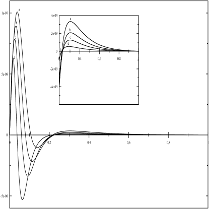
Figure 1: $\delta\hat{R}$ as a function of $x$ for $n=1$, $h=1.5$ and $\Gamma=1.6$. Curves a, b, c and d correspond to $\alpha=.83,\ .85,\ .87\ \mbox{and}\ .90$, respectively.

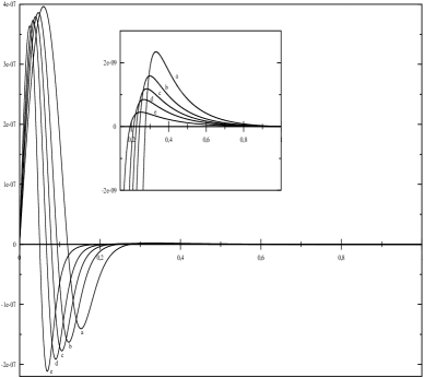
Figure 2: $\delta\hat{R}$ as a function of $x$ for $n=1$, $h=.5$ and $\Gamma=1$. Curves a, b, c, d and e correspond to $\alpha=.80,\ .83,\ .85,\ .87\ \mbox{and}\ .90$, respectively.

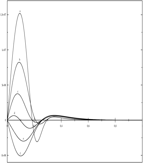
Figure 3: $\delta\hat{R}$ as a function of $x$ for $n=1.5$, $\alpha=.390$, $\Gamma=.6$ and different values of $h$. Curves a, b, c, d, e and f correspond to $h=.5,\ .7,\ .9,\ 1.1,\ 1.3,\ \mbox{and}\ 1.5$, respectively.

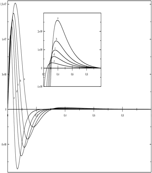
Figure 4: $\delta\hat{R}$ as a function of $x$ for $n=1$, $h=1$ and $\Gamma=1.2$. Curves a, b, c, d and e correspond to $\alpha=.80,\ .83,\ .85,\ .87\ \mbox{and}\ .90$, respectively.

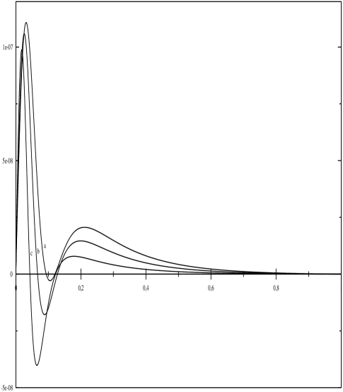
Figure 5: $\delta\hat{R}$ as a function of $x$ for $n=1$, $h=1.5$ and $\Gamma=1.4$. Curves a, b and c correspond to $\alpha=.85,\ .87\ \mbox{and}\ .90$, respectively.

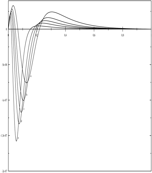
Figure 6: $\delta\hat{R}$ as a function of $x$ for $n=1$, $h=1$ and $\Gamma=.8$. Curves a, b, c, d and e correspond to $\alpha=.80,\ .83,\ .85,\ .87\ \mbox{and}\ .90$, respectively.

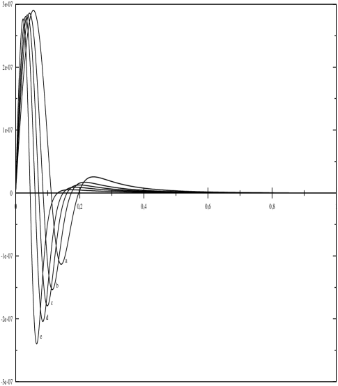
Figure 7: $\delta\hat{R}$ as a function of $x$ for $n=1$, $h=.5$ and $\Gamma=.8$. Curves a, b, c, d and e correspond to $\alpha=.80,\ .83,\ .85,\ .87\ \mbox{and}\ .90$, respectively.

IV Results

We shall now proceed to apply the formalism sketched in the previous section, to detect and analyze the occurrence of cracking in the family of polytropes defined by the equation of state (42). We shall consider both types of polytropes (I and II), and both schemes of perturbation (through $K$ and $h$, and through $n$ and $h$).

To do so, using a four order Runge–Kutta method, we shall integrate (34), (36), and (39), (40), for any duplet of parameters $n,\alpha$ and $n,h$ , for which there exists a boundary surface. Such duplets have been determined in 2p (see figures (3, 4) for the case I, and (8, 9) for the case II, in that reference). Also, the absolute numerical values of the perturbations of the parameters were taken of the order of $10^{-6}$, the results are not qualitatively sensitive, to changes in some orders of magnitude, below or above, that figure. Finally, the integrals (80, 97, 115, 117) were numerically evaluated by means of the trapezoid rule (see for example trap ).

Next, the obtained $\Psi,\Psi_{0}$ (which of course coincide with the results in 2p ) are used to evaluate (83) and (98) for the case I, and (114) and (116) for the case II. We have considered the whole range of values of the parameters leading to bounded configurations, whose physical variables satisfy the physical requirements (31).

We shall now analyze the obtained results for each case.

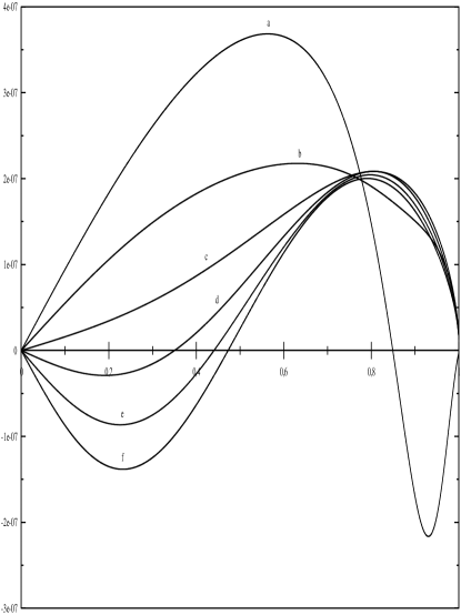
Figure 8: $\delta\hat{R}$ as a function of $x$ for $n=.5$, $\alpha=.98$, $\Gamma=.6$ and different values of $h$. Curves a, b, c, d, e and f correspond to $h=.5,\ .7,\ .9,\ 1.1,\ 1.3,\ \mbox{and}\ 1.5$, respectively.

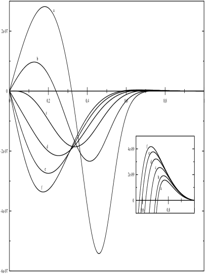
Figure 9: $\delta\hat{R}$ as a function of $x$ for $n=1.5$, $\alpha=.84$, $\Gamma=1.1$ and different values of $h$. Curves a, b, c, d, e and f correspond to $h=.5,\ .7,\ .9,\ 1.1,\ 1.3,\ \mbox{and}\ 1.5$, respectively.

Figure 10: $\delta\hat{R}$ as a function of $x$ for $n=.5$, $h=.5$ and $\Gamma=.6$. Curves a, b, c, d, e and f correspond to $\alpha=.95,\ .96,\ .97,\ .98,\ .99\ \mbox{and}\ 1.00$, respectively.

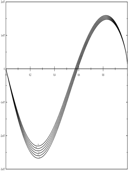
Figure 11: $\delta\hat{R}$ as a function of $x$ for $n=.5$, $h=1.5$ and $\Gamma=.4$. Curves a, b, c, d, e and f correspond to $\alpha=.95,\ .96,\ .97,\ .98,\ .99\ \mbox{and}\ 1.00$, respectively.

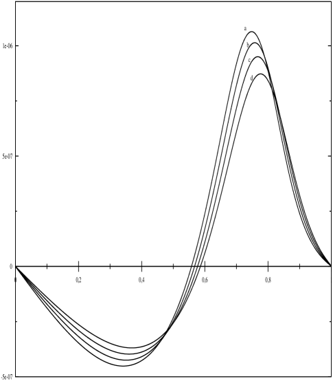
Figure 12: $\delta\hat{R}$ as a function of $x$ for $n=1$, $h=.5$ and $\Gamma=-0.5$. Curves a, b, c, and d correspond to $\alpha=1.0,\ .9,\ .8,\ \mbox{and}\ .7$, respectively.

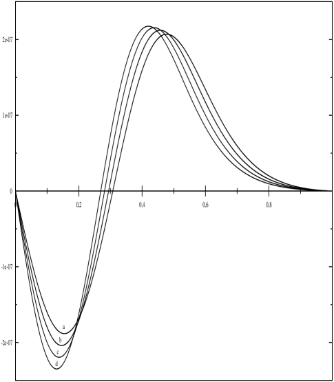
Figure 13: $\delta\hat{R}$ as a function of $x$ for $n=1.5$, $h=1$ and $\Gamma=-0.5$. Curves a, b, c, and d correspond to $\alpha=.7,\ .8,\ .9,\ \mbox{and}\ 1.0$, respectively.

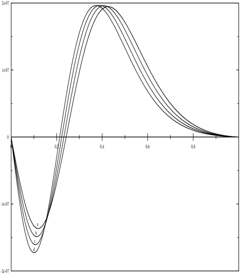
Figure 14: $\delta R$ as a function of $x$ for $n=1.5$, $h=1.5$ and $\Gamma=-0.5$.Curves a, b, c, and d correspond to $\alpha=.7,\ .8,\ .9,\ \mbox{and}\ 1.0$, respectively.

IV.1 Cracking for polytropes of type I

Figures (1–7) summarize the main results obtained for the polytropes of type I. The first four figures (figs. (1–4)) correspond to the case where the perturbation is carried on through the parameter $K$, whereas the remaining three figures of this case (figs.(5–7)) describe the behaviour of the system which has been perturbed through the parameter $n$.

In figure 1 we observe the cracking fo $h=1.5$ and the different values of $\alpha$ indicated in the figure legend. It appears that the strongest, and deepest, crackings are associated with the largest values of $\alpha$. We also observe that in the outer regions, the models exhibit overturnings. In these latter cases, smallest values of $\alpha$ are associated with strongest overturnings.

Figure 2 depicts a similar situation, but for $h=.5$. However in this case crackings are stronger and overturnings are weaker.

The situation described in figures 1 and 2 is representative for a wide range of parameteres (for which there exist bounded configurations satisfying the required physical conditions).

Figure 3 exhibits further the close relationship, existing between the occurrence of cracking and the type of anisotropy. Indeed, the smallest values of $h$ correspond to the deepest and strongest crackings, and to the weakest overturnings. Furthermore, for the largest values of $h$ (curves e and f) there are not crackings at all, only overturnings.

Finally figure 4 exhibits the occurrence of cracking for configurations that are locally isotropic before perturbation, thereby illustrating the fact that even slight deviations from local isotropy, may be sufficient to produce a cracking.

Figures 5–7, which describe the results of perturbation through the parameter $n$, lead to conclusions qualitatively similar to the ones mentioned above. The strongest and deepest crackings, and the weakest overturnings, are associated with largest values of $\alpha$

IV.2 Cracking for polytropes of type II

The results of this case are depicted by figures (8–14). The first four of these, correspond to the perturbative scheme through the parameter $K$ whereas the last three correspond to perturbations of $n$.

Figure 8 describes the situation, for different values of $h$. For the choice of parameters in this figure, we observe that cracking only appears for the smallest value of $h$, whereas for the two largest values, there is only overturning. For $h=.7;.9$ neither cracking nor overturning occurs.

This behaviour is confirmed in figure 9. Here we see how the strongest and deepest crackings are associated with the smallest values of $h$. For some minimal value of $h$, and larger, only overturnings are observed. These are strongest for the largest values of $h$.

Figures 10 and 11 also confirm the role of $h$ in the occurrence (or not) of crackings. In figure 10, for $h=.5$, there are only crackings, which are strongest and deepest for the largest values of $\alpha$. In contrast, figure 11 only depicts overturnings for $h=1.5$ and different values of $\alpha$.

Figures 12, 13 and 14 describe the situation resulting from the perturbation of $n$. However, unlike the previous cases, for these three figures we have assumed negative values of $\Gamma$. This explains why they only exhibit overturnings, and why these overturnings are stronger for smaller values of $h$ (just the opposite of the situation observed for positive values of $\Gamma$).

V Conclusions

We have investigated the conditions under which, general relativistic polytropes for anisotropic matter, exhibit cracking and/or overturning, when submitted to fluctuations of energy density and anisotropy.

Thus, we have shown that cracking and/or overturning occur for a wide range of the parameters. For both types of polytropes, the main conclusions are basically the same, namely: the strongest and deepest crackings occur for the smallest values of $h$ and greatest values of $\alpha$. Also, the strongest overturnings result from the largest values of $h$.

A distinct feature of all the models studied here, is the fact that the “core” (the inner part), and the “envelope” (the outer part), respond differently to different degrees of anisotropy (different $h$). This fact was already pointed out in 2p ; HRW .

It is important to stress that the occurrence of a cracking, has direct implications on the structure and evolution of the compact object, only at time scales that are smaller than, or at most, equal to, the hydrostatic time scale. This is so because as already mentioned, what we do is to take a “snapshot” just after the system leaves the equilibrium. To find out whether or not the system will return to the state of equilibrium afterward, is out of the scope of our analysis, and would require an integration of the evolution equations for a finite period of time, greater than the hydrostatic time.

However, all this having been said, it is clear that the occurrence of cracking would drastically affect the future structure and evolution of the compact object.

Accordingly, we would like to conclude this work by speculating about possible scenarios where the occurrence of cracking might be invoked, in order to understand the related observational data.

One of these situations could be the collapse of a supermassive star. The occurrence of cracking at the inner core, would certainly change (in some cases probably enhance) the conditions for the ejection of the outer mantle in a supernova event. This will be so for both the “prompt” 33 ; 34 and the “long term” mechanisms 35 ; 36 ; 37 ; 38 .

Also, one is tempted to invoke cracking as the possible origin of quakes in neutron stars 39 ; 40 ; 41 . In fact, large scale crust cracking in neutron stars and their relevance in the occurrence of glitches and bursts of x-rays and gamma rays have been considered in detail by Ruderman (see 42 and references therein).

Evidently, the characteristics of these quakes, and those of the ensuing glitches, would strongly depend on the depth at which the cracking occurs. In this respect it is worth noticing, the already mentioned fact, that the depth at which the cracking may appear, is highly dependent on the parameter $h$, which measures the anisotropy of the pressure.

However we would like to emphasize that our aim here is not to model in detail any of the scenarios mentioned above, but just to call attention to the possible occurrence of cracking in such important configurations, as those satisfying a polytropic equation of state, and its relationship with fluctuations of local anisotropy. In other words, whatever the origin of the anisotropy would be, or how small it is, cracking may occur, which would drastically affect the outcome of the evolution of the system.

References

- (1) L. Herrera and W. Barreto, Phys. Rev. D 87, 087303, (2013).
- (2) L. Herrera and W. Barreto, Phys. Rev. D 88, 084022, (2013).
- (3) L. Herrera, A. Di Prisco, W. Barreto and J. Ospino, Gen. Relativ. Gravit. 46, 1827 (2014).
- (4) S. Chandrasekhar, An Introduction to the Study of Stellar Structure (University of Chicago, Chicago, 1939).
- (5) M. Schwarzschild Structure and Evolution of the Stars, (Dover, New York), (1958).
- (6) S. L. Shapiro and S. A. Teukolsky, Black Holes, White Dwarfs and Neutron Stars (John Wiley and Sons, New York, 1983).
- (7) R. Kippenhahn and A. Weigert, Stellar Structure and Evolution (Springer Verlag, Berlin, 1990).
- (8) C. Hansen and S. Kawaler Stellar Interiors: Physical Principles, Structure and Evolution, (Springer Verlag, Berlin) (1994)
- (9) A. Kovetz, Astrophys. J., 154, 999 (1968).
- (10) P. Goldreich and S. Weber, Astrophys. J. 238, 991 (1980).
- (11) M. A. Abramowicz, Acta Astron. 33, 313 (1983).
- (12) R. Tooper, Astrophys. J. 140, 434 (1964).
- (13) R. Tooper, Astrophys. J. 142, 1541 (1965).
- (14) R. Tooper, Astrophys. J. 143, 465 (1966).
- (15) S. Bludman, Astrophys. J. 183, 637 (1973).
- (16) U. Nilsson and C. Uggla, Ann. Phys. 286, 292 (2000).
- (17) H. Maeda, T. Harada, H. Iguchi and N. Okuyama, Phys. Rev. D 66, 027501 (2002).
- (18) L. Herrera and W. Barreto, Gen. Relativ. Gravit. 36, 127 (2004).
- (19) X. Y. Lai and R. X. Xu, Astropart. Phys. 31, 128 (2009).
- (20) S. Thirukkanesh and F. C. Ragel, Pramana J. Phys. 78, 687 (2012).
- (21) F. Shojai, M. R,. Fazel, A. Estepenian and M. Kohandel, Eur. Phys. J.C 75, 250 (2015).
- (22) L. Herrera and N. O. Santos, Phys. Rep. 286, 53 (1997).
- (23) L. Herrera, A. Di Prisco, J. Martin, J. Ospino, N. O. Santos, O. Troconis, Phys. Rev. D 69, 084026 (2004).
- (24) L. Herrera, J. Martin, J. Ospino, J. Math. Phys. 43, 4889 (2002).
- (25) L. Herrera, J. Ospino, A. Di Prisco, Phys. Rev. D 77, 027502 (2008).
- (26) L. Herrera, N. O. Santos, A. Wang, Phys. Rev. D 78, 084026 (2008).
- (27) P. H. Nguyen and J. F. Pedraza, Phys. Rev. D 88, 064020 (2013).
- (28) P. H. Nguyen and M. Lingam, Monh. Not. R. Astron. Soc. 436, 2014 (2013).
- (29) J. Krisch and E.N. Glass, J. Math. Phys. 54, 082501 (2013).
- (30) R. Sharma and B. Ratanpal, Int. J. Mod. Phys. D 22,1350074 (2013).
- (31) E. N. Glass, Gen. Relativ. Gravit. 45, 2661 (2013).
- (32) K. P. Reddy, M. Govender and S. D. Maharaj, Gen. Relativ. Gravit. 47, 35 (2015).
- (33) J. C. Kemp, J. B. Swedlund, J. D. Landstreet and J. R. P. Angel, Astrophys. J. 161, L77 (1970).
- (34) G. D. Schmidt and P. S. Schmidt, Astrophys. J. 448, 305 (1995).
- (35) A. Putney, Astrophys. J. 451, L67 (1995).
- (36) D. Reimers, S. Jordan, D. Koester, N. Bade, Th. Kohler and L. Wisotzki, Astron. Astrophys. 311, 572 (1996).
- (37) A. P. Martinez, R. G. Felipe and D. M. Paret, Int. J. Mod. Phys. D 19, 1511 (2010).
- (38) M. Chaichian, S. S. Masood, C. Montonen, A. Perez Martinez and H. Perez Rojas, Phys. Rev. Lett 84, 5261 (2000).
- (39) A. Perez Martinez, H. Perez Rojas and H. J. Mosquera Cuesta, Eur. Phys. J. C 29, 111 (2003).
- (40) A. Perez Martinez, H. Perez Rojas and H. J. Mosquera Cuesta, Int. J. Mod. Phys. D 17, 2107 (2008).
- (41) E. J. Ferrer, V. de la Incera, J. P. Keith, I. Portillo and P. L. Springsteen, Phys. Rev. C. 82, 065802 (2010).
- (42) R. D. Blandford and L. Hernquist, J. Phys. C: Solid State Physics 15, 6233 (1982).
- (43) N. Andersson, G. Comer and K. Glampedakis, Nucl. Phys. A763, 212 (2005).
- (44) B. Sa’d, I. Shovkovy and D. Rischke, Phys. Rev. D 75, 125004 (2007).
- (45) M. Alford and A. Schmitt, AIP Conf. Proc. 964, 256 (2007).
- (46) D. Blaschke and J. Berdermann, arXiv: 0710.5243.
- (47) A. Drago, A. Lavagno and G. Pagliara, Phys. Rev. D 71, 103004 (2005).
- (48) P. B. Jones, Phys. Rev. D 64, 084003 (2001).
- (49) E. N. E. van Dalen and A. E. L. Dieperink, Phys. Rev. C 69, 025802 (2004).
- (50) H. Dong, N. Su and O. Wang, J. Phys. G 34, S643 (2007).
- (51) M. Fjällborg,J. M. Heinzle and C. Uggla, Proc. Cambridge Phil Soc. 143, 731 (2007).
- (52) H. Andréasson, Living Rev. Relativity 14, 4 (2011).
- (53) T. Ramming and G. Rein, SIAM J. Math. Anal. 45, 900 (2013).
- (54) M. Cosenza, L. Herrera, M. Esculpi and L. Witten, J. Math. Phys. 22, 118 (1981).
- (55) L. Herrera, Phys. Lett. A 165, 206 (1992); 188, 402(1994).
- (56) A. Di Prisco, E. Fuenmayor, L. Herrera and V. Varela, Phys. Lett. A 195, 23 (1994).
- (57) A. Di Prisco, L. Herrera, and V. Varela,Gen. Relativ. Gravit. 29, 1239, (1997).
- (58) L. Herrera and V. Varela, Phys. Lett. A 226, 143 (1997).
- (59) H. Abreu, H. Hernandez and L. Nunez, Classical Quantum Grav. 24, 4631 (2007).
- (60) H.Hernandez and L.Nunez,Can. J. Phys. 91, 328, (2013).
- (61) G. Gonzalez, A. Navarro and L.Nunez, J. Phys. Conf. Ser. 600, 012014 (2015).
- (62) G. Gonzalez, A. Navarro and L.Nunez, arXiv:1505.05550.
- (63) M. Azam, S. Mardan and M. Rehman, Astrophys. Space. Sci. 359,14 (2015).
- (64) J. Mimoso, M. Le Delliou and F. Mena, Phys. Rev. D 81,123514 (2010).
- (65) M. Le Delliou, J. Mimoso, F. Mena, M. Fontanini, D. Guariento and E. Abdalla, Phys.Rev.D 88, 027301 (2013).
- (66) J .Mimoso, M. Le Delliou and F. Mena, Phys. Rev. D 88 ,043501 (2013).
- (67) H. Bondi, Proc. R. Soc. A, 281, 39 (1964).
- (68) F. B Hildebrand, Introduction to Numerical Analysis (Dover, New York 1974).
- (69) L. Herrera, G. Ruggeri and L. Witten, Astrophys. J 234, 1094 (1979).
- (70) S. Colgate and H. Johnson, Phys. Rev. Lett. 5, 235 (1960).
- (71) H. Bethe, G. Brown, J. Applegate, and J. Lattimer, Nucl. Phys. A 324, 487 (1979).
- (72) J. Wilson, in Numerical Relativity, J . Le Blanc and R. Bowers, eds. (Jones and Barlett, Boston) (1985).
- (73) H. Bethe and J. Wilson, Astrophys. J. 295, 14 (1985).
- (74) W.D. Arnett, Astrophys. J. 319, 136 (1987).
- (75) A. Burrows, Astrophys. J. 318, 157 (1987).
- (76) M. Ruderman, Nature (London) 223, 597 (1969).
- (77) D. Pines, J. Shaham, and M. Ruderman, Nature (London) 237, 83 (1972).
- (78) J. Shaham, D. Pines, and M. Ruderman, Ann. N.Y. Acad. Sci., 224, 190 (1973).
- (79) M. Ruderman, Astrophys. J. 382 , 587 (1991).