Graphical functions in parametric space

Abstract.

Graphical functions are positive functions on the punctured complex plane ${\mathbb{C}}\setminus\{0,1\}$ which arise in quantum field theory. We generalize a parametric integral representation for graphical functions due to Lam, Lebrun and Nakanishi, which implies the real analyticity of graphical functions. Moreover we prove a formula that relates graphical functions of planar dual graphs.

1. Introduction

One main problem in perturbative quantum field theory is the calculation of Feynman integrals (see e.g. [12]). As a new tool for this task, graphical functions were introduced by the third author in [24]. Basically, these are special classes of massless Feynman integrals (3-point functions) that can be understood as single-valued functions on the punctured complex plane ${\mathbb{C}}\setminus\{0,1\}$. They are powerful tools in multi-loop calculations, see e.g. [5, 22].

A traditional method to study Feynman integrals is to represent them in a parametric version, where one integrates over variables associated to the edges of a Feynman graph [12]. In many cases of interest, these integrals can be computed in terms of multiple polylogarithms, using a method developed by F. Brown [4, 3] and the second author [21, 19]. The combination of graphical functions and this parametric integration (using the formulas derived in this article) has recently provided a breakthrough in the calculation of primitive log-divergent amplitudes of graphs with up to eleven independent cycles (‘loops’) [22].

In a complete quantum field theoretical calculation one encounters naive singularities which are most frequently treated by the ‘dimensional regularization scheme’ which demands the generalization to arbitrary space-time dimensions (away from the classical four dimensions). The parametric representation is the cleanest way to define Feynman integrals in non-integer ‘dimensions’. In this article, we derive fundamental formulas and results for graphical functions in parametric representations for arbitrary dimensions.

Apart from [22], first applications of the results of this article include the calculation of the beta function and field anomalous dimension of minimally subtracted $(4-\varepsilon)$-dimensional $\phi^{4}$ theory to six and seven loops by the third author [25].

1.1. Feynman integrals in position space

A Feynman graph is a graph $G$ with a distinguished subset ${\mathcal{V}}_{G}^{\mathrm{ext}}\subseteq{\mathcal{V}}_{G}$ of external vertices (the remaining vertices ${\mathcal{V}}_{G}^{\mathrm{int}}={\mathcal{V}}_{G}\setminus{\mathcal{V}}_{G}^{\mathrm{ext}}$ are called internal). We often suppress the subscript $G$ and we use roman capital letters for cardinalities, so e.g. ${\mathcal{V}}^{\mathrm{ext}}={\mathcal{V}}_{G}^{\mathrm{ext}}$ and $V^{\mathrm{ext}}=|{\mathcal{V}}^{\mathrm{ext}}|$. We fix the dimension

$$d=2\lambda+2>2$$

and associate to every vertex $v$ of $G$ a $d$-dimensional vector $x_{v}\in{\mathbb{R}}^{d}$. An edge $e$ between vertices $u$ and $v$ corresponds to the quadratic form $Q_{e}$ which is the square of the Euclidean distance between $x_{u}$ and $x_{v}$,

(1.1) $$Q_{e}=\|x_{u}-x_{v}\|^{2}=\sum_{i=1}^{d}(x_{u}^{i}-x_{v}^{i})^{2}.$$

Moreover, every edge $e$ has an edge weight $\nu_{e}\in{\mathbb{R}}$. Then the Feynman integral associated to $G$ in position space is defined as

(1.2) $$f_{G}^{(\lambda)}(x)=\left(\prod_{v\in{\mathcal{V}}^{\mathrm{int}}}\int_{{\mathbb{R}}^{d}}\frac{\mathrm{d}^{d}x_{v}}{\pi^{d/2}}\right)\frac{1}{\prod_{e}Q_{e}^{\lambda\nu_{e}}},$$

where the first product is over all internal vertices of $G$ and the second product is over all edges of $G$. Note that $f_{G}^{(\lambda)}(x)$ is a function of the external vectors $x=(x_{v})_{v\in{\mathcal{V}}^{\mathrm{ext}}}$ which we always assume to be pairwise distinct ($x_{v}\neq x_{w}$ for $v\neq w$).

The convergence of (1.2) is equivalent to two conditions named ‘infrared’ and ‘ultraviolet’ (this weighted analog of [24, Lemma 3.4] rests on power counting [14]):

• The graph $G$ is called ultraviolet convergent if

  (1.3) $$\lambda\nu_{g}<\tfrac{d}{2}(V_{g}-1)$$

  holds for all induced subgraphs $g$ with $|{\mathcal{V}}_{g}\cap{\mathcal{V}}^{\mathrm{ext}}|\leq 1$. Here we write

  $$\nu_{g}=\sum_{e\in{\mathcal{E}}_{g}}\nu_{e}$$

  and denote the sets of vertices and edges of $g$ with ${\mathcal{V}}_{g}$ and ${\mathcal{E}}_{g}$.

• A vertex $v\in{\mathcal{V}}_{g}$ of a subgraph $g$ of $G$ is called $g$-internal if it is internal ($v\in{\mathcal{V}}^{\mathrm{int}}$) and all edges of $G$ which are incident to $v$ also belong to $g$. We write $V_{g}^{\mathrm{int}}$ for the number of such vertices. The graph $G$ is called infrared convergent if

  (1.4) $$\lambda\nu_{g}>\tfrac{d}{2}V_{g}^{\mathrm{int}}$$

  holds for all subgraphs $g$ of $G$ which satisfy $V_{g}^{\mathrm{int}}>0$ and contain only edges which are incident to at least one $g$-internal vertex.

Example 1.1.

In case of the graph $G_{4}$ from figure 1, there are three ultraviolet conditions of the form $\lambda\nu_{e}<\frac{d}{2}$ (one for each edge $e$) and one infrared condition $\lambda\nu_{G_{4}}>\frac{d}{2}$ (from the full subgraph $g=G_{4}$).

1.2. Graphical functions

In the special case of three external vertices, we label them with $0$, $1$ and $z$. Note that $f_{G}^{(\lambda)}$ is invariant under the Euclidean group, so we may translate $x_{0}$ to the origin and rotate $x_{1}$ and $x_{z}$ into the plane ${\mathbb{R}}^{2}\times\{0\}^{d-2}$ which we identify with the complex numbers ${\mathbb{C}}$. The graphical function

$$f_{G}^{(\lambda)}(z)\colon{\mathbb{C}}\setminus\{0,1\}\longrightarrow{\mathbb{R}}_{+}$$

is a parametrization of $f_{G}^{(\lambda)}(x)$ defined in terms of a complex variable $z\neq 0,1$ via

(1.5) $$x_{0}=(0,\ldots,0)^{t},\quad x_{1}=(1,0,\ldots,0)^{t}\quad\text{and}\quad x_{z}=(\operatorname{Re}z,\operatorname{Im}z,0,\ldots,0)^{t}.$$

Graphical functions were introduced in [24] basically as a tool for calculating Feynman periods in $\phi^{4}$ quantum field theory (see also [22, 10, 26]). However, they can also appear in amplitudes and correlation functions, see for example [9].

In [24] ‘completions’ of graphical functions were defined. In this article, however, we use uncompleted graphs.

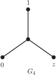
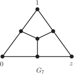
Figure 1. Examples of connected graphs with four and seven vertices in total and three external vertices labeled $0$, $1$ and $z$.

Example 1.2.

In $d=4$ dimensions and with edge weights $\nu_{e}=1$, the graph $G_{4}$ of Figure 1 has a convergent graphical function (see example 1.1). It is (see [24, 26])

$$f_{G_{4}}^{(1)}(z)=\int_{{\mathbb{R}}^{4}}\frac{\mathrm{d}^{4}x}{\pi^{2}}\frac{1}{\|x\|^{2}\|x-x_{1}\|^{2}\|x-x_{z}\|^{2}}=\frac{4{\mathrm{i}}D(z)}{z-{\overline{z}}}$$

in terms of the Bloch-Wigner dilogarithm $D(z)=\operatorname{Im}(\mathrm{Li}_{2}(z)+\log(1-z)\log|z|)$.

The Bloch-Wigner dilogarithm $D(z)$ is a single-valued version of the dilogarithm $\mathrm{Li}_{2}(z)=\sum_{k=1}^{\infty}z^{k}/k^{2}$. It is real analytic on ${\mathbb{C}}\setminus\{0,1\}$ and antisymmetric under complex conjugation $D(z)=-D({\overline{z}})$. These properties of the Bloch-Wigner dilogarithm lift to general properties of graphical functions:

Theorem 1.3.

Let $G$ be a graph which fulfills the ultraviolet and infrared conditions (1.3) and (1.4). Then the graphical function $f_{G}^{(\lambda)}\colon{\mathbb{C}}\setminus\{0,1\}\longrightarrow{\mathbb{R}}_{+}$ has the following general properties:

1. $f_{G}^{(\lambda)}(z)=f_{G}^{(\lambda)}({\overline{z}})$,

2. $f_{G}^{(\lambda)}$ is single-valued and

3. $f_{G}^{(\lambda)}$ is real analytic on ${\mathbb{C}}\setminus\{0,1\}$.

It was not possible to prove real analyticity (G3) in full generality with the methods in [24]. In this article we obtain (G3) as a consequence of an alternative integral representation of graphical functions. In this representation, the integration variables $\alpha_{e}$ (known as Schwinger or Feynman parameters) are associated to edges of the graph [12, 1].

Although we are mainly interested in the case of three external vertices 0, 1, $z$, our results effortlessly generalize to an arbitrary number $V^{\mathrm{ext}}$ of external vertices.

1.3. Graph polynomials

We will use certain polynomials in the edge variables $\alpha_{e}$ that were defined and studied by F. Brown and K. Yeats [6].

Definition 1.4.

Let $p=\{p_{1},\ldots,p_{n}\}$ denote a partition of a subset of the vertices of a graph $G$ (so $p_{i}\subseteq{\mathcal{V}}$ and $p_{i}\cap p_{j}=\emptyset$ when $i\neq j$). We write ${\mathcal{F}}_{G}^{p}$ for the set of all spanning forests $T_{1}\cup\ldots\cup T_{n}$ consisting of exactly $n$ (pairwise disjoint) trees $T_{i}$ such that $p_{i}\subseteq T_{i}$. The dual spanning forest polynomial associated to $p$ is

(1.6) $$\tilde{\Psi}_{G}^{p}(\alpha)\mathrel{\mathop{:}}=\sum_{F\in{\mathcal{F}}_{G}^{p}}\;\prod_{e\in F}\alpha_{e}.$$

We suppress curly brackets in the notation, so for example $\tilde{\Psi}_{G}^{01z}=\tilde{\Psi}_{G}^{\{\{0,1,z\}\}}$ denotes the sum of spanning forests ($n=1$), while the partition in $\tilde{\Psi}_{G}^{01,z}$ is $\{\{0,1\},\{z\}\}$ ($n=2$). Say we call the external vertices $1,\ldots,V^{\mathrm{ext}}$, then we write $\tilde{\Psi}\mathrel{\mathop{:}}=\tilde{\Psi}^{1,\ldots,V^{\mathrm{ext}}}$ for the partition into singletons ($n=V^{\mathrm{ext}}$). The partitions with $n=V^{\mathrm{ext}}-1$ have exactly one part containing two external vertices. We collect them in the polynomial

(1.7) $$\tilde{\Phi}_{G}(\alpha,x)\mathrel{\mathop{:}}=\sum_{1\leq i<j\leq V^{\mathrm{ext}}}\|x_{i}-x_{j}\|^{2}\tilde{\Psi}_{G}^{ij,(k)_{k\neq i,j}}(\alpha).$$

Example 1.5.

If we label the three edges adjacent to $0$, $1$ and $z$ in $G_{4}$ (see Figure 1) by $1$, $2$ and $3$, then we find the polynomials

$$\tilde{\Psi}_{G_{4}}^{1z,0} =\alpha_{2}\alpha_{3}, \tilde{\Psi}_{G_{4}}^{01z} =\alpha_{1}\alpha_{2}\alpha_{3},$$

$$\tilde{\Psi}_{G_{4}}^{0z,1} =\alpha_{1}\alpha_{3}, \tilde{\Psi}_{G_{4}}^{0,1,z} =\alpha_{1}+\alpha_{2}+\alpha_{3},$$

$$\tilde{\Psi}_{G_{4}}^{01,z} =\alpha_{1}\alpha_{2}, \tilde{\Phi}_{G_{4}} =(z-1)({\overline{z}}-1)\alpha_{2}\alpha_{3}+z{\overline{z}}\alpha_{1}\alpha_{3}+\alpha_{1}\alpha_{2}.$$

Here ${\overline{z}}$ denotes the complex conjugate of $z\in{\mathbb{C}}\setminus\{0,1\}$ and we used (1.5).

A parametric (i.e. depending on the edge parameters $\alpha_{e}$) formula for (massive) position space Feynman integrals in four-dimensional Minkowski space was discovered long ago [17, 13] and is also discussed in the book [18, Equation (8-33)]. In the massless, Euclidean case it becomes a parametric formula for graphical functions. We give an extension to arbitrary dimensions which also allows for negative edge weights.

Theorem 1.6.

Let $G$ be a non-empty graph with $V^{\mathrm{int}}_{G}$ internal vertices and edges labeled $1,2,\ldots,E_{G}$. We assume that its graphical function (1.2) converges, meaning that $G$ is subject to (1.3) and (1.4), and define the superficial degree of divergence

(1.8) $$M_{G}\mathrel{\mathop{:}}=\lambda\nu_{G}-\tfrac{d}{2}V^{\mathrm{int}}_{G}.$$

Then for any set of non-negative integers $n_{e}$ such that $n_{e}+\lambda\nu_{e}>0$, we have the following dual parametric representation of $f_{G}^{(\lambda)}$ as a convergent projective integral:

(1.9) $$f_{G}^{(\lambda)}(x)=\frac{(-1)^{\sum_{e}\!n_{e}}\,\Gamma(M_{G})}{\prod_{e}\Gamma(n_{e}+\lambda\nu_{e})}\int_{\Delta}\Omega\Big{[}\prod_{e}\alpha_{e}^{n_{e}+\lambda\nu_{e}-1}\partial_{\alpha_{e}}^{n_{e}}\Big{]}\frac{1}{\tilde{\Phi}_{G}^{M_{G}}\tilde{\Psi}_{G}^{d/2-M_{G}}},$$

where the integration domain is given by the positive coordinate simplex

$$\Delta=\{(\alpha_{1}:\alpha_{2}:\ldots:\alpha_{E_{G}})\colon\alpha_{e}>0\text{ for all }e\in\{1,2,\ldots,E_{G}\}\}\subset{\mathbb{P}}^{E_{G}-1}{\mathbb{R}}$$

and we set

$$\Omega=\sum_{e=1}^{E_{G}}(-1)^{e-1}\alpha_{e}\mathrm{d}\alpha_{1}\wedge\ldots\wedge\widehat{\mathrm{d}\alpha_{e}}\wedge\ldots\wedge\mathrm{d}\alpha_{E_{G}}.$$

Remark 1.7.

For integer $\lambda\nu_{e}\leq 0$ one may set $n_{e}=1-\lambda\nu_{e}$ such that the integration over $\alpha_{e}$ trivializes to the evaluation at $\alpha_{e}=0$ of a $(-\lambda\nu_{e})$’s derivative.

Readers who are not familiar with projective integrals can specialize to an affine integral by setting $\alpha_{1}=1$ and integrating the remaining $\alpha_{e}$ ($e>1$) from $0$ to $\infty$.

Note that $M_{G}$ is restricted by convergence: From (1.4) with $g=G$ and from (1.3) with $g=G\setminus({\mathcal{V}}^{\mathrm{ext}}\setminus\{v\})$ (for some $v\in{\mathcal{V}}^{\mathrm{ext}}$) we obtain for a graph $G$ with no edges between external vertices that

$$0<M_{G}<\lambda\min_{v\in V^{\mathrm{ext}}}\sum_{w\in{\mathcal{V}}^{\mathrm{ext}}\setminus\{v\}}\nu_{w},$$

where $\nu_{w}$ is the sum of weights $\nu_{e}$ of all edges $e$ adjacent to the external vertex $w$.

One immediate advantage of the parametric representation is that for many graphs with not more than nine vertices, the integral (1.10) can be calculated (in terms of polylogarithms) with methods developed by F. Brown [4] and the second author [19, 21].

Note that we obtain another integral representation via the Cremona transformation $\alpha_{e}\rightarrow 1/\alpha_{e}$:

Corollary 1.8.

Let $G$ be a non-empty graph with $E_{G}$ edges. We assume the convergence of $f_{G}^{(\lambda)}$ and also that every edge $e$ has a positive weight $\nu_{e}>0$. Then

(1.10) $$f_{G}^{(\lambda)}(x)=\frac{\Gamma(M_{G})}{\prod_{e}\Gamma(\lambda\nu_{e})}\int_{\Delta}\frac{\prod_{e}\alpha_{e}^{d/2-\lambda\nu_{e}-1}}{\Phi_{G}^{M_{G}}\Psi_{G}^{d/2-M_{G}}}\Omega,$$

where $\Psi_{G}=\Psi_{G}^{1,\ldots,V^{\mathrm{ext}}}$ and $\Phi_{G}(\alpha,x)=\sum_{i<j}\|x_{i}-x_{j}\|^{2}\Psi_{G}^{ij,(k)_{k\neq i,j}}(\alpha)$ are defined in terms of the spanning forest polynomials, which are dual to (1.6):

(1.11) $$\Psi_{G}^{p}(\alpha)=\sum_{F\in{\mathcal{F}}_{G}^{p}}\prod_{e\notin F}\alpha_{e}=\Big{(}\prod_{e}\alpha_{e}\Big{)}\tilde{\Psi}_{G}^{p}(\alpha^{-1}).$$

Proof.

We set $n_{e}=0$ in (1.9) for all edges $e$ of $G$. We use the affine chart $\alpha_{1}=1$ in (1.9) and invert all $\alpha_{e}$, $e>1$. By (1.11) this gives the integrand in (1.10) for $\alpha_{1}=1$. The projective version of this integral is (1.10). ∎

1.4. Planar duals

A planar dual $G^{\star}$ of a Feynman graph $G$ with external vertices $0,1,z$ is a usual planar dual graph to which we add external vertices at ‘opposite’ sides, see Figure 2 (a precise description will be given in Definition 4.1).

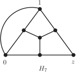
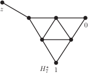
Figure 2. The graphs $H_{7}$ and $H_{7}^{\star}$ are planar duals.

In the case when $M_{G}=d/2$, graphical functions of dual graphs are related:

Theorem 1.9.

Let $G$ be a connected graph with external vertices $0,1,z$ and edge weights $\nu_{e}>0$ such that the graphical function $f_{G}^{(\lambda)}$ converges and $M_{G}=d/2$. Let $G^{\star}$ be a dual of $G$ and denote by $e^{\star}$ the edge of $G^{\star}$ which corresponds to the edge $e$ of $G$. Let the edge weights $\nu_{e^{\star}}$ of $G^{\star}$ be related to the edge weights $\nu_{e}$ of $G$ through

(1.12) $$\lambda\nu_{e^{\star}}=d/2-\lambda\nu_{e}.$$

Then the graphical functions associated to $G$ and $G^{\star}$ are multiples of each other:

(1.13) $$f_{G^{\star}}^{(\lambda)}(z)=f_{G}^{(\lambda)}(z)\prod_{e}\frac{\Gamma(\lambda\nu_{e})}{\Gamma(\lambda\nu_{e^{\star}})}.$$

Note that ultraviolet convergence (1.3) for a single edge $e$ implies $\lambda\nu_{e}<d/2$, thus $\nu_{e}^{\star}>0$. Similarly, positive edge weights in $G$ ensure that the dual graphical function $f_{G^{\star}}^{(\lambda)}$ is ultraviolet convergent for each single edge $e^{\star}$ of $G^{\star}$. The convergence of $f_{G^{\star}}^{(\lambda)}$ is ensured by the proof of Theorem 1.9.

If in four dimensions a graph $G$ has edge weights 1 then a dual graph $G^{\star}$ has also edge weights 1 and the graphical functions are equal if $M_{G}=2$.

One can also use duality for a planar graph $G$ with $M_{G}\neq d/2$ if one adds an edge from 0 to 1 of weight $(d/2-M_{G})/\lambda$, see the subsequent example 1.11.

Remark 1.10.

It is well known (see [16] for example) that the graphical function of every planar graph $G$ (without restrictions on $\nu_{e}$ and $d$) is related (by a constant factor) to the momentum space Feynman integral associated to $G^{\star}$. What makes Theorem 1.9 interesting is that in the particular case when $V^{\mathrm{ext}}=3$ and $M_{G}=d/2$, the momentum- and position space Feynman integrals coincide.

Example 1.11.

We want to calculate the $4$-dimensional graphical function of the graph $G_{7}$ in Figure 1 with unit edge weights, so $M_{G_{7}}=1$. To apply Theorem 1.9 we add an edge between 0 and 1 (see Figure 2). This does not change the graphical function $f_{G_{7}}^{(1)}=f_{H_{7}}^{(1)}$, which is clear from (1.2). Theorem 1.9 gives $f_{H_{7}}^{(1)}=f_{H^{\star}_{7}}^{(1)}$. The graphical function of $H^{\star}_{7}$ can be calculated by the techniques completion and appending of an edge [24, Sections 3.4 and 3.5]. We obtain

$$f_{G_{7}}^{(1)}(z)=20\zeta(5)\frac{4{\mathrm{i}}D(z)}{z-{\overline{z}}},$$

where $\zeta(s)=\sum_{k=1}^{\infty}k^{-s}$ is the Riemann zeta function.

Example 1.12.

One obtains a self dual graph $H_{4}=H_{4}^{\star}$ with $M_{H_{4}}=2$ if one adds an edge from 0 to 1 to $G_{4}$. In this case planar duality leads to a trivial statement.

Acknowledgements.

Parts of this article were written while Erik Panzer and Oliver Schnetz were visiting scientists at Humboldt University, Berlin.

2. proof of Theorem 1.6

Our proof follows the Schwinger trick (see e.g. [12]). From the definition of the gamma function we obtain for $n+\lambda\nu>0$ the convergent integral (note $Q_{e}>0$)

(2.1) $$\frac{1}{Q_{e}^{\lambda\nu_{e}}}=\frac{1}{\Gamma(n_{e}+\lambda\nu_{e})}\int_{0}^{\infty}\alpha_{e}^{n_{e}+\lambda\nu_{e}-1}(-\partial_{\alpha_{e}})^{n}\exp(-\alpha_{e}Q_{e})\ \mathrm{d}\alpha_{e}.$$

We use this formula to replace the product of propagators in (1.2) by an integral over the edge parameters $\alpha_{e}$. Since the integrand $\prod_{e}\big{[}\alpha_{e}^{n_{e}+\lambda\nu_{e}-1}Q_{e}^{n_{e}}\exp(-\alpha_{e}Q_{e})\big{]}$ is positive, the integral is absolutely convergent and we may interchange the order of integration by Fubini’s theorem. In fact, we can also interchange the integration over the vertex variables with the partial derivatives $\partial_{\alpha_{e}}$ to obtain

(2.2) $$f_{G}^{(\lambda)}(x)=\frac{1}{\prod_{e}\Gamma(n_{e}+\lambda\nu_{e})}\int_{0}^{\infty}\!\!\!\cdots\int_{0}^{\infty}\Big{[}\prod_{e}\alpha^{n_{e}+\lambda\nu_{e}-1}(-\partial_{\alpha_{e}})^{n_{e}}\Big{]}{\mathcal{I}}(\alpha)\prod_{e}\mathrm{d}\alpha_{e},$$

where ${\mathcal{I}}(\alpha)$ is the Gaußian integral

$${\mathcal{I}}(\alpha)=\left(\prod_{v\,{\rm internal}}\int_{{\mathbb{R}}^{d}}\frac{\mathrm{d}^{d}x_{v}}{\pi^{d/2}}\right)\exp\left(-\sum_{e}\alpha_{e}Q_{e}\right).$$

It factorizes into $d$ parts ${\mathcal{I}}_{k}$, one for each coordinate $k$, since the quadratic form (1.1) is diagonal. We arrange the $i$th coordinates of the $V_{G}$ vertex variables to the vector $(x_{\mathrm{int}},x_{\mathrm{ext}})^{t}$ where $x_{\mathrm{int}}=(x_{v}^{k})_{v\in{\mathcal{V}}^{\mathrm{int}}}$ and $x_{\mathrm{ext}}=(x_{v}^{k})_{v\in{\mathcal{V}}^{\mathrm{ext}}}$. Then, the quadratic form in the exponential of ${\mathcal{I}}_{k}$ takes the form

$$\sum_{e}\alpha_{e}Q_{e}^{k}=x^{t}_{\mathrm{int}}L^{\mathrm{ii}}(\alpha)x_{\mathrm{int}}+x^{t}_{\mathrm{int}}L^{\mathrm{ie}}(\alpha)x_{\mathrm{ext}}+x_{\mathrm{ext}}^{t}L^{\mathrm{ei}}(\alpha)x_{\mathrm{int}}+x_{\mathrm{ext}}^{t}L^{\mathrm{ee}}(\alpha)x_{\mathrm{ext}}$$

in terms of the (symmetric) Laplace matrix [2]

(2.3) $$L=\begin{pmatrix}L^{\mathrm{ii}}&L^{\mathrm{ie}}\\ L^{\mathrm{ei}}&L^{\mathrm{ee}}\\ \end{pmatrix}\quad\text{with entries}\quad L(\alpha)_{uv}=\begin{cases}\sum\limits_{e{\rm\,incident\,to\,}v}\alpha_{e}&\text{if $u=v$ and}\\ -\sum\limits_{e=\{u,v\}}\alpha_{e}&\text{otherwise.}\end{cases}$$

By convergence, $L^{\mathrm{ii}}$ is positive definite. We complete the quadratic form to a perfect square, shift the integration variable to $x_{\mathrm{int}}+L^{\mathrm{ii}-1}L^{\mathrm{ie}}x_{\mathrm{ext}}$ and obtain by a standard calculation

$${\mathcal{I}}_{k}=\det(L^{\mathrm{ii}})^{-1/2}\exp\Big{(}x_{\mathrm{ext}}^{t}[L^{\mathrm{ei}}L^{\mathrm{ii}-1}L^{\mathrm{ie}}-L^{\mathrm{ee}}]x_{\mathrm{ext}}\Big{)}.$$

The summation over $k$ in the exponent therefore leads us to

(2.4) $${\mathcal{I}}(\alpha)=\prod_{k=1}^{d}{\mathcal{I}}_{k}(\alpha)=\det(L^{\mathrm{ii}})^{-d/2}\exp\Big{(}\sum_{k,\ell=1}^{V^{\mathrm{ext}}}(x_{k}^{t}x_{\ell})[L^{\mathrm{ei}}L^{\mathrm{ii}-1}L^{\mathrm{ie}}-L^{\mathrm{ee}}]_{k,\ell}\Big{)}.$$

An application of the matrix tree theorems [7, 2] shows that

$$\det(L^{\mathrm{ii}})=\tilde{\Psi}\quad\text{and}\quad\left(L^{\mathrm{ii}-1}\right)_{v,w}=\frac{1}{\tilde{\Psi}}\tilde{\Psi}_{G}^{vw,1,\ldots,V^{\mathrm{ext}}}$$

for all internal $v$ and $w$. We can therefore interpret the matrix elements

(2.5) $$\tilde{\Psi}(L^{\mathrm{ei}}L^{\mathrm{ii}-1}L^{\mathrm{ie}})_{k,\ell}=\sum_{\begin{subarray}{c}e=\{k,v\}\\ f=\{\ell,w\}\end{subarray}}\alpha_{e}\alpha_{f}\tilde{\Psi}_{G}^{vw,1,\ldots,V^{\mathrm{ext}}}\quad\text{($v,w$ internal)}$$

in the exponential of (2.4) in terms of subgraphs of $G$. We distinguish two cases:

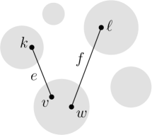
$k\neq\ell$:             $k=\ell$:  

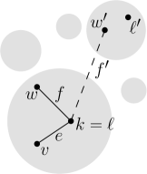
Figure 3. For $k\neq\ell$, the grey areas indicate the connected components of $F$. Adding $e$ and $f$ connects $k$ with $\ell$. In the case $k=\ell$ we depict the connected components of $F^{\prime}=F\cup\{e\}$; note that $w$ lies in the same component as $k$. When we extend the sum to all edges $f$ incident to $k$, additional contributions arise when $w$ lies in a different component of $F^{\prime}$ and thus connects $k$ to another external vertex $\ell^{\prime}$ (indicated by the dashed edge $f^{\prime}$).

• Adding the two edges $e$, $f$ to a spanning forest $F\in{\mathcal{F}}_{G}^{vw,1,\ldots,V^{\mathrm{ext}}}$ yields a forest $F^{\prime}=F\cup\{e,f\}\in{\mathcal{F}}_{G}^{k\ell,(m)_{m\neq k,\ell}}$ (see Figure 3). Conversely, each $F^{\prime}$ arises exactly once this way, because it determines $e$ and $f$ as the initial and final edges on the unique path in $F^{\prime}$ connecting $k$ and $\ell$. The only exception are forests $F^{\prime}$ where this path is just a single edge $e=\{k,\ell\}$ connecting them directly. But in this case $F^{\prime}\setminus e\in{\mathcal{F}}_{G}^{1,\ldots,V^{\mathrm{ext}}}$, so we conclude

  $$\sum_{\mathclap{\begin{subarray}{c}e=\{k,v\}\\ f=\{\ell,w\}\end{subarray}}}\alpha_{e}\alpha_{f}\tilde{\Psi}_{G}^{vw,1,\ldots,V^{\mathrm{ext}}}(\alpha)=\tilde{\Psi}_{G}^{k\ell,(m)_{m\neq k,\ell}}(\alpha)-\tilde{\Psi}\sum_{\mathclap{e=\{k,\ell\}}}\alpha_{e}.$$

• Adding $e$ to $F\in{\mathcal{F}}_{G}^{vw,1,\ldots,V^{\mathrm{ext}}}$ gives a forest $F^{\prime}=F\cup\{e\}\in{\mathcal{F}}_{G}^{1,\ldots,kw,\ldots,V^{\mathrm{ext}}}$. Each such $F^{\prime}$ occurs exactly once, because $e$ is necessarily the (unique) first edge on the path in $F^{\prime}$ connecting $k$ with $w$, hence

  $$(\tilde{\Psi}L^{\mathrm{ei}}L^{\mathrm{ii}-1}L^{\mathrm{ie}})_{k,k}=\sum_{f=\{k,w\}}\alpha_{f}\tilde{\Psi}_{G}^{1,\ldots,kw,\ldots,V^{\mathrm{ext}}}.$$

  For a fixed $F^{\prime}\in{\mathcal{F}}_{G}^{1,\ldots,kw,\ldots,V^{\mathrm{ext}}}$, $f$ runs over all edges that connect $k$ to a vertex $w$ that lies in the same connected component of $F^{\prime}$. If we sum instead over all edges incident to $k$, we get additional contributions when $w$ lies in another component, say the one containing $\ell^{\prime}$ (see Figure 3). Therefore,

  $$(\tilde{\Psi}L^{\mathrm{ei}}L^{\mathrm{ii}-1}L^{\mathrm{ie}})_{k,k}=\tilde{\Psi}\sum_{k\in f}\alpha_{f}-\sum_{\ell^{\prime}\neq k}\tilde{\Psi}_{G}^{k\ell^{\prime},(m)_{m\neq k,\ell^{\prime}}}.$$

According to (2.3), the contributions proportional to $\tilde{\Psi}$ cancel in both cases when we subtract $(\tilde{\Psi}L^{\mathrm{ee}})_{k,\ell}$ from (2.5), such that (2.4) becomes

$${\mathcal{I}}=\tilde{\Psi}^{-d/2}\exp\Big{(}-\tilde{\Psi}^{-1}\sum_{\mathclap{1\leq k<\ell\leq V^{\mathrm{ext}}}}(x_{k}^{2}-2x_{k}^{t}x_{\ell}+x_{\ell}^{2})\tilde{\Psi}_{G}^{k\ell,(m)_{m\neq k,\ell}}\Big{)}=\tilde{\Psi}^{-d/2}\exp(-\tilde{\Phi}_{G}/\tilde{\Psi}).$$

Let us now insert a factor $1=\int_{0}^{\infty}\delta(t-H^{1/r}(\alpha))\mathrm{d}t$ into (2.2), where $H(\alpha)$ can be any homogeneous polynomial of degree $r>0$ which is positive inside $\Delta$. After we substitute all $\alpha_{e}$ by $t\alpha_{e}$ and collect the powers of $t$, the integrand of (2.2) becomes

$$\delta(1-H^{1/r}(\alpha))\Big{(}\prod_{e}\alpha_{e}^{n_{e}+\lambda\nu_{e}-1}\partial_{\alpha_{e}}^{n_{e}}\Big{)}\tilde{\Psi}^{-d/2}\Big{[}\int_{0}^{\infty}t^{M_{G}-1}\mathrm{e}^{-t\tilde{\Phi}_{G}/\tilde{\Psi}}\mathrm{d}t\Big{]}\prod_{e}\mathrm{d}\alpha_{e},$$

because $\tilde{\Psi}$ and $\tilde{\Phi}_{G}$ are homogeneous in $\alpha$ of degree $V^{\mathrm{int}}$ and $V^{\mathrm{int}}+1$, respectively. We integrate over $t$ using (2.1). The choice $H(\alpha)=\alpha_{e}$ for some edge $e$ gives a particularly simple representation as an affine integral over ${\mathbb{R}}_{+}^{E_{G}-1}$ which is equivalent to (1.9).

3. proof of Theorem 1.3

In this section we prove the real analyticity of graphical functions. Because the polynomial $\tilde{\Phi}_{G}$ from (1.7) depends on the squared distances

$$s_{i,j}=\|x_{i}-x_{j}\|^{2}$$

between the external vertices, we may use the dual parametric representation (1.9) to define $f_{G}^{(\lambda)}(s)$ as a function of the vector $s=(s_{i,j})_{1\leq i<j\leq V^{\mathrm{ext}}}$. In the (simply connected) domain where all components of $s$ have positive real parts, the integral (1.9) remains absolutely convergent and hence $f_{G}^{(\lambda)}(s)$ an analytic function of $s$:

Theorem 3.1.

Let $G$ be a graph with a convergent graphical function (1.2). Then $f_{G}^{(\lambda)}(x)$ extends to a single-valued, analytic function

$$f_{G}^{(\lambda)}(s)\colon\big{\{}s\in{\mathbb{C}}^{V^{\mathrm{ext}}(V^{\mathrm{ext}}-1)/2}\colon\text{$\operatorname{Re}s_{i,j}>0$ for all $1\leq i<j\leq V^{\mathrm{ext}}$}\big{\}}\longrightarrow{\mathbb{C}}.$$

In the special case of three external vertices, this implies the real analyticity of $f_{G}^{(\lambda)}(z)$ on ${\mathbb{C}}\setminus\{0,1\}$:

Proof of Theorem 1.3.

Let $z\in{\mathbb{C}}\setminus\{0,1\}$. For the three external labels $0$, $1$, $z$ we have $s_{0,1}=1>0$, $s_{0,z}=z{\overline{z}}>0$ and $s_{1,z}=(z-1)({\overline{z}}-1)>0$ according to (1.5). With theorem 3.1 we see that $f_{G}^{(\lambda)}(z,\bar{z})$ is composition of analytic functions, which proves (G3). The identity (G1) is immediate from (1.9) as it expresses $f_{G}^{(\lambda)}(z)$ as a function of $|z|$ and $|1-z|$. Finally recall that $f_{G}^{(\lambda)}(z)$ is defined as the value of the (convergent) integral (1.2) and thus manifestly single-valued. ∎

For the proof of Theorem 3.1 we need the following notation:

Definition 3.2.

Let $g$ be a subgraph of $G$ with edge set ${\mathcal{E}}_{g}\subseteq{\mathcal{E}}_{G}$ and let $Q\in{\mathbb{C}}[\alpha_{e},e\in{\mathcal{E}}_{G}]$ be a polynomial in the edge variables of $G$. Then, the (low) degree ($\underline{\operatorname{deg}}_{g}(Q)$) $\deg_{g}(Q)$ of $Q$ is the (low) degree of $Q$ in the edge variables $\alpha_{e}$, $e\in{\mathcal{E}}_{g}$ of the subgraph $g$.

In other words, $c=\underline{\operatorname{deg}}_{g}(Q)$ is the largest integer such that each monomial in $Q$ has at least $c$ factors $\alpha_{e}$ with $e\in{\mathcal{E}}_{g}$ (with multiplicity). Similarly, $C=\deg_{g}(Q)$ is the smallest integer such that each monomial in $Q$ has at most $C$ factors $\alpha_{e}$ with $e\in{\mathcal{E}}_{g}$.

Note that $\underline{\operatorname{deg}}_{g}(Q)$ and $\deg_{g}(Q)$ are defined for polynomials $Q$ in $E_{G}$ variables. So for $Q=\alpha_{1}-\alpha_{3}+\alpha_{2}$ we have $\underline{\operatorname{deg}}_{\{2\}}(Q)=0$, even though on the subspace $\alpha_{1}=\alpha_{3}$ the low degree of $Q$ in $\alpha_{2}$ is 1.

Proposition 3.3.

Let $g$ be a subgraph of a graph $G$ with external vertices. Let $\tilde{\Psi}^{p}_{G}(\alpha)$ be a dual spanning forest polynomial (1.6) for some partition $p$ of external vertices. Then

(3.1) $$\underline{\operatorname{deg}}_{g}(\tilde{\Psi}^{p}_{G})\geq V^{\mathrm{int}}_{g},\quad\deg_{g}(\tilde{\Psi}^{p}_{G})\leq V_{g}-1,$$

where ${\mathcal{V}}_{g}$ and $V^{\mathrm{int}}_{g}$ are as in (1.3) and (1.4), respectively.

Proof.

Let $F\in{\mathcal{F}}^{p}_{G}$ be a spanning forest of $G$. In every tree $T$ of $F$ we choose an external vertex $v_{T}\in T$ and we orient all edges of $T$ such that they point towards $v_{T}$. Because $F$ is spanning, every $g$-internal vertex $u$ has one outgoing edge in $F$. Conversely, every edge in $F$ has a unique vertex $u$ as source, therefore

$$\underline{\operatorname{deg}}_{g}(\tilde{\Psi}^{p}_{G})=\min_{F\in{\mathcal{F}}^{p}_{G}}E_{g\cap F}\geq V^{\mathrm{int}}_{g}.$$

Finally we use that $g\cap F$ is a forest in $g$ and thus has at most $V_{g}-1$ edges, hence

$$\deg_{g}(\tilde{\Psi}^{p}_{G})=\max_{F\in{\mathcal{F}}^{p}_{G}}E_{g\cap F}=V_{g}-1.\qed$$

Proof of Theorem 3.1.

We first derive Theorem 3.1 from (1.9) in the case that all $n_{e}=0$. We consider the integrand as a function of the vector $s=(s_{i,j})_{i,j\in{\mathcal{V}}^{\mathrm{ext}},i<j}$ which we restrict to the complex domain ($\varepsilon>0$ may be chosen arbitrarily small)

$$\Omega^{\varepsilon}=\left\{s\colon\operatorname{Re}s_{i,j}>\varepsilon\quad\text{for all $1\leq i<j\leq V^{\mathrm{ext}}$}\right\}\subset{\mathbb{C}}^{V^{\mathrm{ext}}(V^{\mathrm{ext}}-1)/2}.$$

Let $\hat{s}_{i,j}=\|\hat{x}_{i}-\hat{x}_{j}\|^{2}$ denote the distances of an arbitrary set $\hat{x}\in{\mathbb{R}}^{dV^{\mathrm{ext}}}$ of pairwise distinct points. We can rescale $\hat{x}$ to ensure $\max_{i<j}(\hat{s}_{i,j})=\varepsilon$, such that

$$|\tilde{\Phi}_{G}(\alpha,s)|\geq\operatorname{Re}\tilde{\Phi}_{G}(\alpha,s)>\tilde{\Phi}_{G}(\alpha,\hat{x})$$

for every $s\in\Omega^{\varepsilon}$ and all $\alpha\in{\mathbb{R}}_{+}^{E}$. As $f^{(\lambda)}_{G}(\hat{x})$ is convergent, its parametric integrand provides an integrable majorant $F(\alpha,\hat{s})\geq F(\alpha,s)$ to the integrand $F(\alpha,s)$ of $f_{G}^{(\lambda)}(s)$, uniformly for all $s\in\Omega^{\varepsilon}$. This implies the analyticity of $f_{G}^{(\lambda)}(s)$ in $\Omega^{\varepsilon}$, for every $\varepsilon>0$ (we cite this result below as theorem 3.4).

Now let us remove the restriction that $n_{e}=0$. We compute the derivatives in (1.9) and write the resulting integrand as

(3.2) $$F(\alpha,s)=\left[\prod_{e}\alpha_{e}^{n_{e}+\lambda\nu_{e}-1}\right]\frac{\sum_{m}\alpha^{m}q_{m}(s)}{\tilde{\Phi}_{G}(\alpha,s)^{M_{G}+\sum_{e}n_{e}}\tilde{\Psi}(\alpha)^{d/2-M_{G}+\sum_{e}n_{e}}},$$

where we expanded the numerator polynomial into its monomials $\alpha^{m}=\prod_{e}\alpha_{e}^{m_{e}}$ in Schwinger parameters and their coefficients $q_{m}\in{\mathbb{Q}}[s_{i,j}]$. Note that the operators $\alpha_{e}\partial_{\alpha_{e}}$ do not change the $\alpha$-degree, so $F$ stays homogeneous of degree $-E_{G}$ in the $\alpha$ variables, no matter which values are chosen for the $n_{e}$. This gives

$$\sum_{e}m_{e}=\left(\deg_{G}(\tilde{\Phi}_{G})+\deg_{G}(\tilde{\Psi}_{G})-1\right)\sum_{e}n_{e}=2V^{\mathrm{int}}\sum_{e}n_{e},$$

because the polynomials $\tilde{\Phi}_{G}$ and $\tilde{\Psi}_{G}$ have the $\alpha$-degrees $V^{\mathrm{int}}+1$ and $V^{\mathrm{int}}$. If we write (3.2) as $F(\alpha,s)=\sum_{m}q_{m}(s)F_{m}(\alpha,s)$ we can thus identify each $F_{m}$ with the (dual parametric) integrand for $f^{(\lambda^{\prime})}_{G}(s)$ in $d^{\prime}=2\lambda^{\prime}+2=d+4\sum_{e}n_{e}$ dimensions with weights $\lambda^{\prime}\nu_{e}^{\prime}=\lambda\nu_{e}+n_{e}+m_{e}>0$. With the first part of the proof it suffices to show that each of these $f^{(\lambda^{\prime})}_{G}$ is a convergent graphical function. We therefore have to consider the infrared (1.4) and ultraviolet (1.3) conditions. Because differentiation $\partial_{\alpha_{e}}$ for $e\in{\mathcal{E}}_{g}$ can lower the low degree by at most one, we obtain

$$\sum_{e\in g}m_{e}-(\underline{\operatorname{deg}}_{g}(\tilde{\Phi}_{G})+\underline{\operatorname{deg}}_{g}(\tilde{\Psi}_{G}))\sum_{e\in G}n_{e}\geq-\sum_{e\in g}n_{e}.$$

From the convergence of $f^{(\lambda)}_{G}$ and from Proposition 3.3 we obtain

$$\sum_{e\in g}\lambda^{\prime}\nu_{e}^{\prime}=\sum_{e\in g}(\lambda\nu_{e}+n_{e}+m_{e})>\tfrac{d}{2}V_{g}^{\mathrm{int}}+2V_{g}^{\mathrm{int}}\sum_{e\in G}n_{e}=\tfrac{d^{\prime}}{2}V_{g}^{\mathrm{int}},$$

proving infrared convergence. Likewise, differentiation $\partial_{\alpha_{e}}$ for $e\in{\mathcal{E}}_{g}$ lowers the degree by at least one, yielding

$$\sum_{e\in g}m_{e}-(\deg_{g}(\tilde{\Phi}_{G})+\deg_{g}(\tilde{\Psi}_{G}))\sum_{e\in G}n_{e}\leq-\sum_{e\in g}n_{e}.$$

Together with Proposition 3.3 this proves ultraviolet convergence (and thus completes our proof of Theorem 3.1):

$$\sum_{e\in g}\lambda^{\prime}\nu_{e}^{\prime}=\sum_{e\in g}(\lambda\nu_{e}+n_{e}+m_{e})<\left(\tfrac{d}{2}+2\sum_{e\in G}n_{e}\right)(V_{g}-1)=\tfrac{d^{\prime}}{2}(V_{g}-1).\qed$$

For convenience of the reader we cite here the result from calculus in the form [23, Theorem 2.12], which is perfectly adapted to our application:

Theorem 3.4.

Let $\Theta\subset{\mathbb{R}}^{m}$ and $\Omega\subset{\mathbb{C}}^{n}$ denote domains in the respective spaces of dimensions $m,n\in{\mathbb{N}}$. Furthermore, let

$$f(t,z)=f(t_{1},\ldots,t_{m},z_{1},\ldots,z_{n})\colon\Theta\times\Omega\longrightarrow{\mathbb{C}}$$

represent a continuous function with the following properties:

• For each fixed $t\in\Theta$, the function $z\mapsto f(t,z)$ is holomorphic in $z\in\Omega$.

• We have a continuous function $F(t)\colon\Theta\longrightarrow[0,\infty)$ which is integrable,

  $$\int_{\Theta}F(t)\ \mathrm{d}t<\infty,$$

  and uniformly majorizes $f$: $|f(t,z)|\leq F(t)$ for all $(t,z)\in\Theta\times\Omega$.

Then the function $z\mapsto\int_{\Theta}f(t,z)\ \mathrm{d}t$ is holomorphic in $\Omega$.

Remark 3.5.

We may consider a graphical function $f_{G}^{(\lambda)}(z)$ as a function of two complex variables $z$ and ${\overline{z}}$ and analytically continue away from the locus where ${\overline{z}}$ is the complex conjugate of $z$. In this case Theorem 3.1 states that $f_{G}^{(\lambda)}$ is analytic in $z$ and ${\overline{z}}$ if $\operatorname{Re}z{\overline{z}}>0$ and $\operatorname{Re}(1-z)(1-{\overline{z}})>0$. If one continues analytically beyond this domain, additional singularities will in general appear. Already in example 1.2 we encounter $z=\bar{z}$, which corresponds to the vanishing of the Källén function

$$(z-{\overline{z}})^{2}=s_{0,z}^{2}+s_{1,z}^{2}+s_{0,1}^{2}-2s_{0,z}s_{1,z}-2s_{0,z}s_{0,1}-2s_{1,z}s_{0,1}.$$

For bigger graphs the singularity structure outside $\operatorname{Re}z{\overline{z}}>0$, $\operatorname{Re}(1-z)(1-{\overline{z}})>0$ becomes more and more complicated (see [20, table 1] for a few examples).

4. proof of Theorem 1.9

Planar duality for graphical functions is specific to three external labels for which we use $0$, $1$, $z$. Let us first recall the notion of planarity and planar duality for Feynman graphs in this case.

Definition 4.1.

Let $G$ be a graph with three external labels $0$, $1$, $z$. Let $G_{v}$ be the graph that we obtain from $G$ by adding an extra vertex $v$ which is connected to the external vertices of $G$ by edges $\{0,v\}$, $\{1,v\}$, $\{z,v\}$, respectively. We say that $G$ is externally planar if and only if $G_{v}$ is planar.

Let $G_{v}$ be planar and $G_{v}^{\star}$ a planar dual of $G_{v}$. The edges $e^{\star}$ of $G_{v}^{\star}$ are in one to one correspondence with the edges $e$ of $G_{v}$. A planar dual of $G$ is given by $G_{v}^{\star}$ minus the triangle $\{0,v\}^{\star}$, $\{1,v\}^{\star}$, $\{z,v\}^{\star}$ with external labels $0$, $1$, $z$ corresponding to the faces $1zv$, $0zv$, $01v$, respectively. The edge weights of $G^{\star}$ are related to the edge weights of $G$ by (1.12): $\lambda\nu_{e}+\lambda\nu_{e^{\star}}=d/2$.

We can draw an externally planar graph $G$ with the external labels 0, 1, $z$ in the outer face. A dual $G^{\star}$ then has also the labels in the outer face, ‘opposite’ to the labels of $G$, see Figure 2.

Another way to construct this dual is by adding three edges $e_{01}=\{0,1\}$, $e_{0z}=\{0,z\}$, $e_{1z}=\{1,z\}$ to $G$ to obtain a graph $G_{e}$. Its dual $G_{e}^{\star}$ differs from $G_{v}^{\star}$ upon replacing the triangle $\{0,v\}^{\star}$, $\{1,v\}^{\star}$, $\{z,v\}^{\star}$ by a star $e_{01}^{\star}$, $e_{0z}^{\star}$, $e_{1z}^{\star}$. From $G_{e}^{\star}$ we obtain $G^{\star}$ by removing this star and labeling its tips with $z$, $1$, $0$, respectively. Clearly both constructions (starting from the same planar embedding of $G$) lead to the same dual $G^{\star}$ and prove

Lemma 4.2.

Let $G$ be externally planar with dual $G^{\star}$. Then $G^{\star}$ is externally planar and $G$ is a dual of $G^{\star}$.

Proof of Theorem 1.9.

Because the edge weights are positive we can use $n_{e}=0$ in (1.9). From $M_{G}=d/2$ we obtain (see (1.8) and (1.12))

$$M_{G^{\star}}=\sum_{e}(\tfrac{d}{2}-\lambda\nu_{e})-\tfrac{d}{2}V^{\mathrm{int}}_{G^{\star}}=\tfrac{d}{2}(E_{G}-V^{\mathrm{int}}_{G^{\star}}-V^{\mathrm{int}}_{G}-1)=\tfrac{d}{2}(E_{G_{v}}-V_{G_{v}^{\star}}-V_{G_{v}}+3)$$

where $E_{G}$ is the number of edges of $G$. As the vertices of $G_{v}^{\star}$ are the faces of the planar embedding of $G_{v}$, Euler’s formula for planar graphs shows $M_{G^{\star}}=d/2$.

Comparing (1.9) for the graph $G$ with (1.10) for the graph $G^{\star}$ leads to (1.13) if we identify $\alpha_{e}=\alpha_{e^{\star}}$ for all edges $e$, provided that $\tilde{\Phi}_{G}=\Phi_{G^{\star}}$. This amounts to the identity $\tilde{\Psi}^{ij,k}_{G}=\Psi^{ij,k}_{G^{\star}}$ of spanning forest polynomials for all triples $\{i,j,k\}=\{0,1,z\}$ and hence follows from the bijection of 2-forests given by

$${\mathcal{F}}^{ij,k}_{G}\ni F\longleftrightarrow F^{\star}:=\{e^{\star}\colon e\not\in F\}\in{\mathcal{F}}^{ij,k}_{G^{\star}}.$$

Namely, for any given $F\in{\mathcal{F}}^{ij,k}_{G}$ consider the spanning tree $T_{i}=F\cup\{\{i,v\},\{k,v\}\}$ of $G_{v}$. As Tutte points out [27, Theorem 2.64], its dual $T_{i}^{\star}=\{e^{\star}\colon e\notin T\}\subseteq{\mathcal{E}}_{G_{v}^{\star}}$ is a spanning tree of $G_{v}^{\star}$ and therefore, $F^{\star}=T_{i}^{\star}\setminus\{j,v\}^{\star}$ is indeed a $2$-forest. Furthermore, the edge $\{j,v\}^{\star}$ connects the external vertices $i$ and $k$ of $G^{\star}$ and thus $F^{\star}$ cannot connect $i$ with $k$ (otherwise, $T_{i}^{\star}=F^{\star}\cup\{j,v\}^{\star}$ would contain a cycle). Likewise (interchanging $i$ and $j$) $F^{\star}$ does not connect $j$ with $k$, hence $F^{\star}\in{\mathcal{F}}^{i,k}_{G^{\star}}\cap{\mathcal{F}}^{j,k}_{G^{\star}}={\mathcal{F}}^{ij,k}_{G^{\star}}$. Finally, the symmetry $F=(F^{\star})^{\star}$ implies that the map $F\mapsto F^{\star}$ is injective and onto. ∎

References

- [1] S. Bloch, H. Esnault and D. Kreimer, On motives associated to graph polynomials, Commun. Math. Phys. 267 (2006), no. 1 pp. 181–225, arXiv:math/0510011.
- [2] C. Bogner and S. Weinzierl, Feynman graph polynomials, International Journal of Modern Physics A 25 (2010) pp. 2585–2618, arXiv:1002.3458 [hep-ph].
- [3] F. C. S. Brown, The massless higher-loop two-point function, Commun. Math. Phys. 287 (May, 2009) pp. 925–958, arXiv:0804.1660 [math.AG].
- [4] F. C. S. Brown, “On the periods of some Feynman integrals.” preprint, Oct., 2009, arXiv:0910.0114 [math.AG].
- [5] F. C. S. Brown and O. Schnetz, Single-valued multiple polylogarithms and a proof of the zig-zag conjecture, Journal of Number Theory 148 (Mar., 2015) pp. 478–506, arXiv:1208.1890 [math.NT].
- [6] F. C. S. Brown and K. A. Yeats, Spanning forest polynomials and the transcendental weight of Feynman graphs, Commun. Math. Phys. 301 (Jan., 2011) pp. 357–382, arXiv:0910.5429 [math-ph].
- [7] S. Chaiken, A combinatorial proof of the all minors matrix tree theorem, SIAM Journal on Algebraic Discrete Methods 3 (Sept., 1982) pp. 319–329.
- [8] E. B. Curtis, D. Ingerman and J. A. Morrow, Circular planar graphs and resistor networks, Linear Algebra and its Applications 283 (Nov., 1998) pp. 115–150.
- [9] J. Drummond, C. Duhr, B. Eden, P. Heslop, J. Pennington and V. A. Smirnov, Leading singularities and off-shell conformal integrals, JHEP 8 (Aug., 2013) p. 133, arXiv:1303.6909 [hep-th].
- [10] J. M. Drummond, Generalised ladders and single-valued polylogs, Journal of High Energy Physics 2013 (Feb., 2013) p. 92, arXiv:1207.3824 [hep-th].
- [11] J. Elstrodt, Maß- und Integrationstheorie. Springer-Lehrbuch. Berlin: Springer, 7 ed., 2011.
- [12] C. Itzykson and J.-B. Zuber, Quantum Field Theory. Dover Publications, Inc., 2006. first published by McGraw-Hill in 1980.
- [13] C. S. Lam and J. P. Lebrun, Feynman-parameter representations for momentum- and configuration-space diagrams, Il Nuovo Cimento A Series 10 59 (Feb., 1969) pp. 397–421.
- [14] J. H. Lowenstein and W. Zimmermann, The power counting theorem for Feynman integrals with massless propagators, Commun. Math. Phys. 44 (1975), no. 1 pp. 73–86.
- [15] L. Mattner, Complex differentiation under the integral, Nieuw. Arch. Wisk. 5/2 (Mar., 2001) pp. 32–35.
- [16] M. Minami and N. Nakanishi, Duality between the Feynman integral and a perturbation term of the Wightman function, Progress of Theoretical Physics 40 (July, 1968) pp. 167–177.
- [17] N. Nakanishi, Feynman-parametric formula for the Hankel-transformed position-space Feynman integral, Progress of Theoretical Physics 42 (Oct., 1969) pp. 966–977.
- [18] N. Nakanishi, Graph theory and Feynman integrals, vol. 11 of Mathematics and its applications. Gordon and Breach, New York, 1971.
- [19] E. Panzer, Feynman integrals and hyperlogarithms. PhD thesis, Humboldt-Universität zu Berlin, 2014. arXiv:1506.07243 [math-ph].
- [20] E. Panzer, On hyperlogarithms and Feynman integrals with divergences and many scales, JHEP 2014 (Mar., 2014) p. 71, arXiv:1401.4361 [hep-th].
- [21] E. Panzer, Algorithms for the symbolic integration of hyperlogarithms with applications to Feynman integrals, Computer Physics Communications 188 (Mar., 2015) pp. 148–166, arXiv:1403.3385 [hep-th].
- [22] E. Panzer and O. Schnetz, “The Galois coaction on periods.” to appear in Communications in Number Theory and Physics, 2016, arXiv:1603.04289 [hep-th].
- [23] F. Sauvigny, Partial differential equations 1. Springer, Berlin, second ed., 2012.
- [24] O. Schnetz, Graphical functions and single-valued multiple polylogarithms, Communications in Number Theory and Physics 8 (2014), no. 4 pp. 589–675, arXiv:1302.6445 [math.NT].
- [25] O. Schnetz, “Numbers and functions in quantum field theory.” preprint, 2016, arXiv:1606.08598 [hep-th].
- [26] I. Todorov, Polylogarithms and multizeta values in massless Feynman amplitudes, in Lie Theory and Its Applications in Physics (V. Dobrev, ed.), vol. 111 of Springer Proceedings in Mathematics & Statistics, pp. 155–176. Springer Japan, 2014.
- [27] W. T. Tutte, Lectures on matroids, J. Res. Nat. Bur. Standards Sect. B 69B (1965), no. 1–2 pp. 1–47. reprinted in: Selected papers of W. T. Tutte, Vol. II (D. McCarthy, R. G. Stanton, eds.), Charles Babbage Research Centre, St. Pierre, Manitoba, 1979, pp. 439–496.