Fluctuations of harmonic and radial flow in heavy ion collisions with principal components

Abstract

We analyze the spectrum of harmonic flow, $v_{n}(p_{T})$ for $n=0\text{--}5$, in event-by-event hydrodynamic simulations of Pb+Pb collisions at the CERN Large Hadron Collider (${\sqrt{s_{\scriptscriptstyle NN}}}=2.76\,{\rm TeV}$) with principal component analysis (PCA). The PCA procedure finds two dominant contributions to the two-particle correlation function. The leading component is identified with the event plane $v_{n}(p_{T})$, while the subleading component is responsible for factorization breaking in hydrodynamics. For $v_{0}$, $v_{1}$, and $v_{3}$ the subleading flow is a response to the radial excitation of the corresponding eccentricity. By contrast, for $v_{2}$ the subleading flow in peripheral collisions is dominated by the nonlinear mixing between the leading elliptic flow and radial flow fluctuations. In the $v_{2}$ case, the sub-sub-leading mode more closely reflects the response to the radial excitation of $\varepsilon_{2}$. A consequence of this picture is that the elliptic flow fluctuations and factorization breaking change rapidly with centrality, and in central collisions (where the leading $v_{2}$ is small and nonlinear effects can be neglected) the subsub-leading mode becomes important. Radial flow fluctuations and nonlinear mixing also play a significant role in the factorization breaking of $v_{4}$ and $v_{5}$. We construct good geometric predictors for the orientation and magnitudes of the leading and subleading flows based on a linear response to the geometry, and a quadratic mixing between the leading principal components. Finally, we suggest a set of measurements involving three point correlations which can experimentally corroborate the nonlinear mixing of radial and elliptic flow and its important contribution to factorization breaking as a function of centrality.

I Introduction

Two-particle correlation measurements are of paramount importance in studying ultrarelativistic heavy ion collisions, and provide an extraordinarily stringent test for theoretical models. Indeed, the measured two-particle correlations exhibit elliptic, triangular, and higher harmonics flows, which can be used to constrain the transport properties of the quark gluon plasma (QGP) Heinz and Snellings (2013); Luzum and Petersen (2014). The remarkable precision of the experimental data as a function of transverse momentum and pseudorapidity has led to new analyses of factorization breaking, nonlinear mixing, event shape selection, and forward-backward fluctuations Khachatryan et al. (2015); Aad et al. (2014a, 2015); Adam et al. ; Adamczyk et al. (2015); Adare et al. (2015). In this paper we analyze the detailed structure of two-particle transverse momentum correlations by using event-by-event (boost-invariant) hydrodynamics and principal component analysis (PCA) Bhalerao et al. (2015); Mazeliauskas and Teaney (2015). Specifically, we decompose the event-by-event harmonic flow $V_{n}(p_{T})$ into principal components and investigate the physical origin of each of these fluctuations. This paper extends our previous analysis Mazeliauskas and Teaney (2015) for triangular flow at the LHC (Pb+Pb at ${\sqrt{s_{\scriptscriptstyle NN}}}=2.76\,{\rm TeV}$) to the other harmonics, $n=0\text{--}5$. In particular, we demonstrate the importance of radial flow fluctuations for subleading flows of higher harmonics.

Taking the second harmonic for definiteness, the two-particle correlation matrix of momentum dependent elliptic flows, $C_{2}(p_{T1},p_{T2})\equiv\left\langle V_{2}(p_{T1})V_{2}^{*}(p_{T2})\right\rangle$ is traditionally parametrized by $r_{2}(p_{T1},p_{T2})$ Gardim et al. (2013),

$$r_{2}(p_{T1},p_{T2})\equiv\frac{\left\langle V_{2}(p_{T1})V_{2}^{*}(p_{T2})\right\rangle}{\sqrt{\left\langle|V_{2}(p_{T1})|^{2}\right\rangle\left\langle|V_{2}(p_{T2})|^{2}\right\rangle}}\,.$$ (1)

If there is only one source of elliptic flow in the event [for example if in each event $V_{2}(p_{T})=f(p_{T})\varepsilon_{2}$ with $\varepsilon_{2}$ a complex eccentricity and $f(p_{T})$ a fixed real function of $p_{T}$] then the correlation matrix of elliptic flows $C_{2}(p_{T1},p_{T2})$ factorizes into a product of functions, and the $r_{2}$ parameter is unity. However, if there are multiple independent sources of elliptic flow in the event, then the correlation matrix does not factorize, and the $r_{2}$ parameter is less than unity Gardim et al. (2013). The $r_{2}$ parameter has been extensively studied both experimentally Khachatryan et al. (2015); Aamodt et al. (2012); Aad et al. (2012, 2014b) and theoretically Gardim et al. (2013); Heinz et al. (2013); Kozlov et al. ; Mazeliauskas and Teaney (2015). In particular, in our prior work on triangular flow we showed that factorization breaking in event-by-event hydrodynamics arises because the simulated triangular flow is predominantly the result of two statistically uncorrelated contributions—the linear response to $\varepsilon_{3}$ Alver et al. and the linear response to the first radial excitation of $\varepsilon_{3}$ Mazeliauskas and Teaney (2015). The goal of the current paper is to extend this understanding of factorization breaking to the other harmonics. This extension was surprisingly subtle due to the quadratic mixing between the leading and subleading harmonic flows.

Experimentally, it is observed that factorization breaking is largest for elliptic flow in central collisions (see in particular Fig. 28 of Ref. Aad et al. (2012) and Fig. 1 of Ref. Khachatryan et al. (2015)). Indeed, the $r_{2}$ parameter decreases rather dramatically from mid-central to central collisions. This indicates that the relative importance of the various initial state fluctuations which drive elliptic flow are changing rapidly as a function of centrality. The current manuscript explains the rapid centrality dependence of factorization breaking in $v_{2}$ as an interplay between the linear response to the fluctuating elliptic geometry, and the nonlinear mixing of the radial flow and average elliptic flow. This quadratic mixing is similar to the mixing between $v_{5}$ and $v_{2},v_{3}$  Borghini and Ollitrault (2006); Qiu and Heinz (2011); Gardim et al. (2012); Teaney and Yan (2012), and this picture can be confirmed experimentally by measuring specific three point correlations analogous to the three plane correlations measured in the $v_{5},v_{2},v_{3}$ case Aad et al. (2014a, 2015).

To understand the linear and nonlinear contributions quantitatively, we will break up the fluctuations in hydrodynamics into their principal components, and analyze the linear and nonlinear contributions of each principal component to the simulated harmonic spectrum. The sample of events and most of the PCA methods are the same as in our previous paper Mazeliauskas and Teaney (2015), and therefore in Sects. II.1 and II.2 we only briefly review the analysis definitions, and the key features of simulations. In Sect. II.3 we discuss the strategy for constructing the best linear predictor for leading and subleading flows.

The second part of our paper, Sect. III, contains individual discussions for each harmonic flow. First, we discuss radial flow fluctuations in Sect. III.1 and then demonstrate their importance in generating subleading elliptic flow in Sect. III.2.1. In Sect. III.3 we briefly describe our PCA results for direct and triangular flows. Finally, in Sect. III.4 we discuss the quadrangular and pentagonal flows and how the nonlinear mixing of lower order principal components adds to these flows. We put forward some experimental observables in the discussion in Sect. IV. A catalog of figures showing the main results of PCA for each harmonic is given in the Appendix.

II PCA of two-particle correlations in event-by-event hydrodynamics

II.1 Principal components

PCA is a statistical technique for extracting the dominant components in fluctuating data. In the context of flow in heavy ion collisions it was first introduced in Ref. Bhalerao et al. (2015), and then applied to the analysis of triangular flow in our previous paper Mazeliauskas and Teaney (2015). Here we review the essential definitions.

The event-by-event single particle distribution is customarily expanded in a Fourier series

$$\frac{dN}{d{\bf p}}=V_{0}(p_{T})+\sum_{n=1}^{\infty}V_{n}(p_{T})e^{-in\varphi}+{\rm H.c.}\,,$$ (2)

where $d{\bf p}=dy\,dp_{T}\,d\varphi$ denotes the phase space, $\varphi$ is the azimuthal angle of the distribution, and H.c. denotes Hermitian conjugate. $V_{n}(p_{T})$ is a complex Fourier coefficient recording the magnitude and orientation of the $n$th harmonic flow, without the typical normalization by multiplicity.

PCA is done by expanding the covariance matrix of two-particle correlations (which is real, symmetric, and positive semi-definite) into real orthogonal eigenvectors $V_{n}^{(a)}(p_{T})$,

$$C_{n}(p_{T1},p_{T2}) \equiv\big{<}\big{(}V_{n,p_{T1}}-\left<V_{n,p_{T1}}\right>\big{)}\big{(}V^{*}_{n,p_{T2}}-\left<V^{*}_{n,p_{T2}}\right>\big{)}\big{>}$$

$$=\sum_{a}V_{n}^{(a)}(p_{T1})V^{(a)}_{n}(p_{T2}),$$ (3)

where $V_{n}^{(a)}=\sqrt{\lambda_{a}}\psi^{(a)}(p_{T})$ is the square root of the eigenvalue times a normalized eigenvector. The eigenvalue records the squared variance of a given fluctuation.

The principal components $V_{n}^{(1)}(p_{T}),V_{n}^{(2)}(p_{T}),\ldots$ of a given event ensemble can be used as optimal basis for event-by-event expansion of harmonic flow

$$V_{n}(p_{T})-\left<V_{n}(p_{T})\right>=\xi_{n}^{(1)}V^{(1)}_{n}(p_{T})+\xi_{n}^{(2)}V^{(2)}_{n}(p_{T})+\ldots\,.$$ (4)

The complex coefficients $\xi_{n}^{(a)}$ are the projections of harmonic flow onto principal component basis and record the orientation and event-by-event amplitude of their respective flows. Principal components are mutually uncorrelated

$$\left<\xi_{n}^{(a)}\xi_{n}^{*(b)}\right>=\delta^{ab}.$$ (5)

Typically the eigenvalues of $C_{n}(p_{T1},p_{T2})$ are strongly ordered and only the first few terms in the expansion are significant. Often the large components have a definite physical interpretation. We define the scaled magnitude of the flow vector $V_{n}^{(a)}(p_{T})$ as

$$\|v^{(a)}_{n}\|^{2}\equiv\frac{\int\big{(}V_{n}^{(a)}\!(p_{T})\big{)}^{2}dp_{T}}{\int\left<dN/dp_{T}\right>^{2}dp_{T}},$$ (6)

which is a measure of the size of the fluctuation without trivial dependencies on the mean multiplicity in a given centrality class.

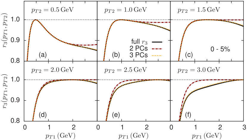
Figure 1: Factorization ratio $r_{3}(p_{T1},p_{T2})$ [Eq. (7)] for triangular flow and its approximations with principal components (PCs) in central collisions (0–5%).

The leading flow vector $V^{(1)}_{n}(p_{T})$ corresponds to fluctuations with the largest root-mean-square amplitude, while subsequent components maximize the variance in the remaining orthogonal directions. This yields a very efficient description of the full covariance matrix $C_{n}(p_{T1},p_{T2})$ and factorization ratio

$$r_{n}(p_{T1},p_{T2})\equiv\frac{C_{n}(p_{T1},p_{T2})}{\sqrt{C_{n}(p_{T1},p_{T1})C_{n}(p_{T2},p_{T2})}}\leq 1\,.$$ (7)

$r_{n}(p_{T1},p_{T2})$ is bounded by unity within hydrodynamics Gardim et al. (2013). By truncating series expansion of the covariance matrix [Eq. (3)] at two or three principal components we can approximate $C_{n}(p_{T1},p_{T2})$ and $r_{n}(p_{T1},p_{T2})$. Truncating at the leading term would constitute complete flow factorization, i.e., $r_{n}=1$. The factorization matrix for triangular flow is shown in Fig. 1. We see that at low momentum $p_{T}<2\,\rm{GeV}$ just two principal components are sufficient to describe momentum dependence of factorization ratio $r_{3}$. Analogous decompositions of two-particle correlations into principal components exist for all harmonics and all centralities. Interpreting these large flow components physically is the goal of this paper.

II.2 Simulations

We used boost-invariant event-by-event viscous hydrodynamics to simulate 5000 Pb-Pb collisions at the CERN Large Hadron Collider (LHC) (${\sqrt{s_{\scriptscriptstyle NN}}}=2.76\,{\rm TeV}$) in fourteen 5% centrality classes selected by impact parameter. The initial conditions are based on the Phobos Glauber Monte Carlo Alver et al. with a two-component model for the entropy distribution in the transverse plane. We used a lattice equation of state Laine and Schroder (2006) and a “direct” pion freeze-out at $T_{\rm fo}=140\,{\rm MeV}$. The results presented here were simulated using a shear viscosity to entropy ratio of $\eta/s=0.08$. Qualitatively similar results are obtained with $\eta/s=0.16$, with the most important differences discussed in Sect. III.2.2. The same ensemble of events was used in Ref. Mazeliauskas and Teaney (2015), which provides further simulation details.

II.3 Geometrical predictors

We will construct several geometric predictors for the leading and subleading flows following strategy outlined in Ref. Gardim et al. (2012). Keeping the discussion general, let $\xi^{(a)}_{n\,\text{pred}}$ be a geometric quantity which predicts the event-by-event amplitude and phase of the corresponding flow $\xi^{(a)}_{n}$ . For example, for the leading $n=3$ component the triangularity $\varepsilon_{3,3}$ (defined below) is an excellent choice for $\xi_{3\,\text{pred}}^{(1)}$.

The geometric predictors are designed to maximize the correlation between a particular flow signal and the geometry. Specifically, the predictors maximize the Pearson correlation coefficient between the event-by-event magnitude and orientation of $a$th principal component, $\xi^{(a)}_{n}$, and the geometrical predictor $\xi^{(a)}_{n\,\text{pred}}$

$$\text{max}\quad Q^{(a)}_{n}=\frac{\big{<}\xi^{(a)}_{n}\xi^{*(a)}_{n\,\text{pred}}\big{>}}{\sqrt{\big{<}\xi^{(a)}_{n}{\xi^{*}_{n}}^{(a)}\big{>}\big{<}\xi^{(a)}_{n\,\text{pred}}\xi^{*(a)}_{n\,\text{pred}}\big{>}}}.$$ (8)

We constructed several predictors for the flow $\xi^{(a)}_{n}$ by assuming a linear relation between the flow and the geometry. The simplest predictor consists of linear combinations of the first two eccentricities of the initial geometry. These are defined as

$$\varepsilon_{n,n} \equiv-\frac{[r^{n}e^{in\phi}]}{R_{\rm rms}^{n}}\,,$$ (9a)

$$\varepsilon_{n,n+2} \equiv-\frac{[r^{n+2}e^{in\phi}]}{R_{\rm rms}^{n+2}}\,,$$ (9b)

where the square brackets $[\,]$ denote an integral over the initial entropy density for a specific event, normalized by the average total entropy $\bar{S}_{\text{tot}}$. $R_{\rm rms}\equiv\sqrt{\left\langle[r^{2}]\right\rangle}$ is the event averaged root-mean-square radius. Note that our definitions of $\varepsilon_{n,n}$ and $\varepsilon_{n,n+2}$ are chosen to make the event-by-event quantities $\varepsilon_{n,n}$ and $\varepsilon_{n,n+2}$ linear in the fluctuations. In this notation, the geometric predictor based on these eccentricities is

$$\xi_{n\,\text{pred}}^{(a)}=\varepsilon_{n,n}+c_{1}\,\varepsilon_{n,n+2},$$ (10)

where $c_{1}$ is adjusted to maximize the correlation coefficient in Eq. (8), and the overall normalization is irrelevant. While the first two eccentricities provide an excellent predictor for the leading flow, they do not predict the subleading flow very well. This is in part because the radial weight $r^{n+2}$ is too strong at large $r$.

More generally, one can define eccentricity as a functional of radial weight function $\rho(r)$:

$$\varepsilon_{n}\{\rho(r)\}\equiv-\frac{[\rho(r)e^{in\phi}]}{R_{\text{rms}}^{n}}.$$ (11)

It is the goal of this paper to find the optimal radial weight function $\rho(r)$ for predicting both leading and subleading flows. For the subleading modes $\rho(r)$ will have a node, and thus $\varepsilon_{n}\{\rho(r)\}$ will measure the magnitude and orientation of the first radial excitation of the geometry Mazeliauskas and Teaney (2015).

To find the optimal radial weight we expand $\rho(r)$ in radial Fourier modes

$$\rho(r)=\sum_{b=1}^{n_{k}}w_{b}\frac{2^{n}n!}{k_{b}^{n}}J_{n}(k_{b}r),$$ (12)

where $J_{n}(x)$ is a Bessel function of order $n$, $w_{b}$ are expansion coefficients, and $k_{b}$ are definite wavenumbers specified below. The prefactor is chosen so that for a single $k$ mode ($w_{1}=1,w_{b>1}=0$) at small $k$ ($kR_{\rm rms}\ll 1$) the generalized eccentricity approaches $\varepsilon_{n,n}$

$$\lim_{k\rightarrow 0}\varepsilon_{n}\{\rho(r)\}=\varepsilon_{n,n}.$$ (13)

At small $k$, we expand the $J_{n}(kr)$ and find

$$\varepsilon_{n}\{\rho(r)\}\simeq\varepsilon_{n,n}+c_{1}\,\varepsilon_{n,n+2},$$ (14)

where $c_{1}=-(kR_{\rm rms}/2)^{2}/(1+n)$. Thus the functional form of $\rho(r)$ adopted here yields a tunable linear combination of the eccentricities in Eq. (9), but the wave number parameter regulates the behavior at large $r$. Further motivation and discussion of this basis set for $\rho(r)$ is given in our previous work Mazeliauskas and Teaney (2015).

We have found that an approximately optimal radial weight can be found by using only two well chosen $k_{b}$ values for the Fourier expansion in Eq. (12). Including additional $k$ modes in the functional form of $\rho(r)$ does not significantly improve the predictive power of the generalized geometric eccentricity. For the two $k$ modes we required (somewhat arbitrarily) that the ratio of $k$ values would be fixed to the ratio of the first two Bessel zeros:

$$\frac{k_{1}}{k_{2}}=\frac{j_{n,1}}{j_{n,2}}\,.$$ (15)

With this choice our basis functions were orthogonal in the interval $[0,R_{o}]$, where $k_{1}=j_{n,1}/R_{o}$. We then adjusted $R_{o}$ to maximize the correlation coefficient between $\varepsilon_{n}\{\rho(r)\}$ and the flow $\xi^{(a)}_{n}$. To account for changing system size with centrality, we used a fixed $R_{o}/R_{\text{rms}}$ ratio. In most cases we used $R_{o}/R_{\text{rms}}\approx 3.0$, but for all directed flow components ($\xi_{1}^{(1)}$ and $\xi_{1}^{(2)}$) and the second elliptic flow component ($\xi_{2}^{(2)}$), we found that $R_{o}/R_{\text{rms}}\approx 2.0$ optimized the correlation between the flow and the geometry.

Ultimately, the assumption that the amplitude and phase of the flow is determined at least approximately by initial eccentricity, $\varepsilon_{n}\{\rho(r)\}$, is based on linear response. If nonlinear physics becomes important (as in the case of $v_{4}$ and $v_{5}$) then the predictors should be modified to incorporate this physics (see below and Ref. Gardim et al. (2012)). Thus, below we will refer to the $\varepsilon_{n}\{\rho(r)\}$ (with an optimized radial weight) as the best linear predictor and incorporate quadratic nonlinear corrections to the predictor as needed.

III Results

III.1 Radial flow

Radial flow (or $V_{0}(p_{T})$) is the first term in the Fourier series and is by far the largest harmonic. Traditionally, the experimental and theoretical study of the fluctuations of $V_{0}(p_{T})$ (i.e., multiplicity and $p_{T}$ fluctuations) has been distinct from elliptic and triangular flow. There is no reason for this distinction.

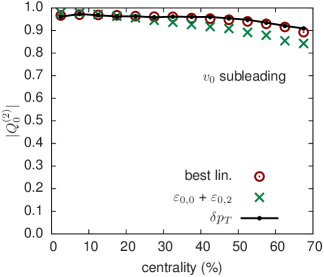
Figure 2: (a) The $p_{T}$ dependence of the principal components of radial flow normalized by the average multiplicity, $v_{0}^{(a)}(p_{T})\equiv V_{0}^{(a)}(p_{T})/\left<dN/dp_{T}\right>$. (b) The Pearson correlation coefficient [Eq. (8)] between the subleading radial flow and various predictors versus centrality. The best linear predictor is described in Sect. II.3.

Examining the scaled $V_{0}(p_{T})$ eigenvalues shown in Fig. 2(a), we see that there are two large principal components. The first principal component is sourced by multiplicity fluctuations, i.e., the magnitude of $V_{0}(p_{T})$ fluctuates (but not its shape) due to the impact parameter variance in a given centrality bin. Corroborating this inference, Fig. 2(a) shows the momentum dependence of the leading principal component, which is approximately flat. Clearly this principal component is not particularly interesting, and the PCA procedure gives a practical method for isolating these trivial geometric fluctuations in the data set. The second principal component is of much greater interest, and shows a linear rise with $p_{T}$ that is indicative of the fluctuations in the radial flow velocity of the fluid Bhalerao et al. (2015).

In early insightful papers Broniowski et al. (2009); Bozek and Broniowski (2012), the fluctuations in the flow velocity (or mean $p_{T}$) were associated with the fluctuations in the initial fireball radius. These radial fluctuations are well described by both the eccentricities $(\varepsilon_{0,0}$, $\varepsilon_{0,2})$, Eq. (9), and the optimized eccentricity $\varepsilon_{0}\{\rho(r)\}$, Eq. (11). Therefore, as seen in Fig. 2(b), the subleading flow signal is strongly correlated with these linear geometric predictors.

Also shown in Fig. 2(b) is the correlation between subleading radial flow $\xi_{0}^{(2)}$ and mean transverse momentum fluctuations around the average

$$\delta p_{T}\equiv[p_{T}]-\left<[p_{T}]\right>.$$ (16)

Indeed, the subleading radial flow correlates very well with mean momentum fluctuations in all centrality bins.

In the next sections we will study the nonlinear mixing between the radial flow $\xi_{0}^{(2)}$ and all other harmonics.

III.2 Elliptic flow

III.2.1 Nonlinear mixing and elliptic flow

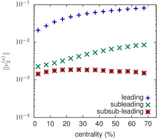
Figure 3: The magnitudes of the principal components of elliptic flow, $\|v^{(a)}_{2}\|$, versus centrality [see Eq. (6)].

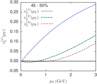
Figure 4: The $p_{T}$ dependence of the principal components of elliptic flow normalized by the average multiplicity, $v_{2}^{(a)}(p_{T})\equiv V_{2}^{(a)}(p_{T})/\left<dN/dp_{T}\right>$, for central (0–5%) and peripheral collisions (45–50%).

We next study the fluctuations of $V_{2}(p_{T})$ as function of centrality. As seen in Fig. 3, the principal component spectrum of elliptic flow in central collisions consists of two nearly degenerate subleading components in addition to the dominant leading component. This degeneracy is lifted in more peripheral bins. Comparing the $p_{T}$ dependence of the principal flows shown in Figs. 4(a) and 4(b), we see that going from central (0–5%) to peripheral (45–50%) collisions, the magnitude of the second principal component increases in size and its momentum dependence changes dramatically. By contrast, the growth of the third principal component is much more mild. This strongly suggests that the average elliptic geometry is more important for the subleading than the subsub-leading mode.

To find a geometrical predictor for the sub- and sub-sub-leading modes we first tried the best linear predictor $\varepsilon_{2}\{\rho(r)\}$. In Fig. 5(a) (the red circles), we see that the correlation coefficient between this optimal linear predictor and the subleading flow signal drops precipitously as a function of centrality. As we will explain now, this is because nonlinear mixing becomes important for the subleading mode.

The ellipticity of the almond shaped geometry in peripheral collisions is traditionally parametrized by eccentricity $\varepsilon_{2,2}$ and it serves as an excellent predictor for the leading elliptic flow. However, $\varepsilon_{2,2}$ does not completely fix the initial geometry, and the radial size of the fireball can fluctuate at fixed eccentricity. As explained in Sect. III.1, the radial size fluctuations modulate the momentum spectrum of the produced particles, and for a background geometry with large constant eccentricity this generates fluctuations in the $p_{T}$ dependence of the elliptic flow, i.e., subleading elliptic flow. This subleading flow lies in the reaction plane following the average elliptic flow, but its sign (which is determined by $\delta p_{T}$) is uncorrelated with $\varepsilon_{2,2}$.

The orientation of the reaction plane in peripheral bins is strongly correlated with the integrated $v_{2}$ or the leading elliptic principal component $\xi_{2}^{(1)}$, while the mean $p_{T}$ fluctuations are tracked by the subleading radial flow component $\xi_{0}^{(2)}$. Therefore we correlated the sub- and sub-sub-leading elliptic flows with the product of the leading elliptic and radial flows, i.e. we computed the correlation coefficient in Eq. (8) with $\xi_{2,\rm pred}^{(2)}=\xi_{2}^{(1)}\xi_{0}^{(2)}$. Examining Fig. 5(a) (the black line), we see see that the correlation between the subleading elliptic flow and the nonlinear mixing rises with centrality, as the correlation with best linear predictor drops. Examining Fig. 5(b) on the other hand, we see that the subsub-leading elliptic flow has stronger correlation with the initial geometry than the nonlinear mixing. Combining best linear geometric predictor and quadratic mixing terms in the predictor, i.e.

$$\xi_{2\,\rm pred}^{(2)}=\varepsilon_{2}\{\rho(r)\}+c_{1}\xi_{2}^{(1)}\xi_{0}^{(2)},$$ (17)

we achieve consistently high correlations for all centralities [the blue diamonds in Fig. 5(a) and (b)].

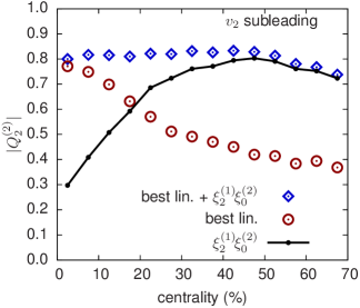
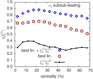
Figure 5: Pearson correlation coefficient between the subleading elliptic flows and the best linear predictor [Eq. (11)] with and without the nonlinear mixing between the radial and leading elliptic flows, $\xi_{2}^{(1)}\xi_{0}^{(2)}$. (a) and (b) show the correlation coefficient for $v_{2}$ subleading and $v_{2}$ subsub-leading flows respectively.

III.2.2 Dependence on viscosity

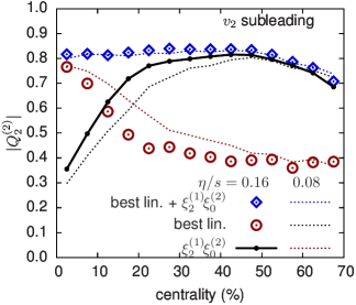
Figure 6: Pearson correlation coefficients for the subleading elliptic flow at viscosity over entropy ratio $\eta/s=0.16$. Dashed lines repeat $\eta/s=0.08$ results from Fig. 5(a) for the ease of comparison.

Before leaving this section we will briefly comment on the viscosity dependence of these results. Figure 6 shows a typical result for a slightly larger shear viscosity, $\eta/s=0.16$. As discussed above, the subleading elliptic flow [i.e., the event-by-event fluctuations in $V_{2}(p_{T})$] is a result of the linear response to the first radial excitation of the elliptic eccentricity, and a nonlinear mixing of radial flow fluctuations and the leading elliptic flow. In Fig. 6 we see that a slightly larger shear viscosity tends to preferentially damp the linear response leaving a stronger nonlinear signal. This is because the initial geometry driving the linear response has a significantly larger gradients due to the combined azimuthal and radial variations. Thus in Fig. 6 the linear response dominates the subleading flow only in very central collisions. These trends with centrality are qualitatively familiar from previous analyses of the effect of shear viscosity on the nonlinear mixing of harmonics Teaney and Yan (2012); Qiu and Heinz (2012).

III.3 Triangular and directed flows

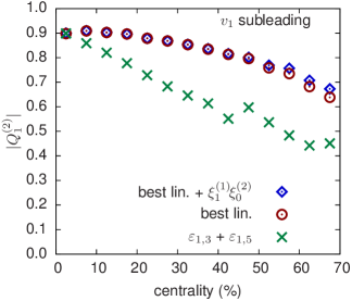
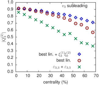
Figure 7: Pearson correlation coefficient between the subleading (a) directed and (b) triangular flows and the best linear predictor with and without radial flow mixing.

Triangular flow was extensively studied in our previous work Mazeliauskas and Teaney (2015). For the sake of completeness we relegate several comparative plots to the Appendix. Previously, we constructed an optimal linear predictor $\varepsilon_{3}\{\rho(r)\}$ for the subleading triangular mode which characterizes the radially excited triangular geometry. As shown in Fig. 7(b), adding the nonlinear mixing term $\xi_{0}^{(2)}\xi_{3}^{(1)}$ to the best linear predictor marginally improves the already good correlation with the subleading flow in peripheral collisions.

Directed flow exhibits many similarities to triangular flow. Specifically the subleading directed flow is reasonably well correlated with the optimal linear predictor, characterizing the radially excited dipolar geometry. Nonlinear mixing between the leading directed flow and the radial flow is unimportant [see Fig. 7(a)].

III.4 The $n=4$ and $n=5$ harmonic flows

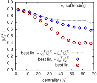
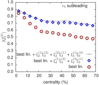
Figure 8: Pearson correlation coefficient between the subleading $v_{4}$ and $v_{5}$ flows and the best linear predictor with and without several nonlinear terms [see Eqs. (21) and (22)].

It is well known that the leading components of the $n=4$ and $n=5$ harmonics are determined by the nonlinear mixing of lower order harmonics in peripheral collisions Borghini and Ollitrault (2006); Qiu and Heinz (2011); Gardim et al. (2012); Teaney and Yan (2012); Aad et al. (2015).

For comparison with other works Gardim et al. (2012, 2015), in the Appendix in Figs. 13(d) and 14(d) we construct a predictor based on a linear combination of the eccentricities

$$\varepsilon_{4,4}+c_{1}\varepsilon_{2,2}\varepsilon_{2,2}\quad\text{for }n=4,$$ (18)

$$\varepsilon_{5,5}+c_{1}\varepsilon_{2,2}\varepsilon_{3,3}\quad\text{for }n=5,$$ (19)

where here and below the coefficient $c_{1}$ is adjusted to maximize the correlation with the flow. This predictor is compared to a linear combination of the optimal eccentricity $\varepsilon_{n}\{\rho(r)\}$ and the corresponding nonlinear mixings of the leading principal components

$$\varepsilon_{4}\left\{\rho(r)\right\}+c_{1}\xi_{2}^{(1)}\xi_{2}^{(1)}\quad\text{for }n=4,$$ (20a)

$$\varepsilon_{5}\left\{\rho(r)\right\}+c_{1}\xi_{2}^{(1)}\xi_{3}^{(1)}\quad\text{for }n=5.$$ (20b)

Both sets of predictors perform reasonably well, though the second set has a somewhat stronger correlation with the flow.

Returning to the subleading components, we first correlated with the best linear predictors, $\varepsilon_{4}\{\rho(r)\}$ and $\varepsilon_{5}\{\rho(r)\}$, with the corresponding subleading flow signals. As seen in Fig. 8 (the red circles), the correlation decreases rapidly with centrality, especially for $v_{4}$. Motivated by Eq. (20) which predicts the event-by-event leading $v_{4}$ and $v_{5}$ in terms $v_{2}$ and $v_{3}$, we construct a predictor for the subleading $v_{4}$ and $v_{5}$ in terms of the fluctuations of $v_{2}$ and $v_{3}$ (see Secs. III.2.1 and III.3, respectively). The full predictor reads

$$\varepsilon_{4}\left\{\rho(r)\right\}+c_{1}\xi_{2}^{(1)}\xi_{2}^{(2)}, \text{for }n=4,$$ (21a)

$$\varepsilon_{5}\left\{\rho(r)\right\}+c_{1}\xi_{2}^{(1)}\xi_{3}^{(2)}+c_{2}\xi_{3}^{(1)}\xi_{2}^{(2)}, \text{for }n=5.$$ (21b)

Including the mixings between the subleading $v_{2}$ and $v_{3}$ and the corresponding leading components greatly improves the correlation in mid-central bins (the blue diamonds). Finally, in an effort to improve the $v_{4}$ predictor in the most peripheral bins we have added additional nonlinear mixings between the radial flow and the leading principal components

$$\varepsilon_{4}\left\{\rho(r)\right\}+c_{1}\xi_{2}^{(1)}\xi_{2}^{(2)}+c_{2}\xi_{4}^{(1)}\xi_{0}^{(2)}, \text{for }n=4,$$ (22a)

$$\varepsilon_{5}\left\{\rho(r)\right\}+c_{1}\xi_{2}^{(1)}\xi_{3}^{(2)}+c_{2}\xi_{3}^{(1)}\xi_{2}^{(2)}+c_{3}\xi_{5}^{(1)}\xi_{0}^{(2)}, \text{for }n=5.$$ (22b)

As seen in Fig. 8(a) (the grey line) the coupling to the radial flow improves the correlation between the subleading $v_{4}$ and the predictor in peripheral collisions. On the other hand, for $v_{5}$, Fig. 8(b), all of the information about the coupling to the radial flow is already included in Eq. (21b) and adding $v_{0}$ does not improve the correlation.

IV Discussion

In this paper we classified the event-by-event fluctuations of the momentum dependent Fourier harmonics $V_{n}(p_{T})$ for $n=0\text{--}5$ by performing a principal component analysis of the two-particle correlation matrix in hydrodynamic simulations of heavy ion collisions. The leading principal component for each harmonic is very strongly correlated with the integrated flow, and therefore this component is essentially the familiar $v_{n}(p_{T})$ measured in the event plane. The subleading components describe additional $p_{T}$ dependent fluctuations of the magnitude and phase of $v_{n}(p_{T})$. This paper focuses on the physical origins of the subleading flows, which are the largest source of factorization breaking in hydrodynamics.

Our systematic study started by placing radial flow (the $n=0$ harmonic) in the same framework as the other harmonic flows. We identified the subleading $n=0$ principal component with mean $p_{T}$ fluctuations and confirmed (as is well known Broniowski et al. (2009); Bozek and Broniowski (2012)) that these fluctuations are predicted by the variance of the radial size of the fireball.

The subleading directed and triangular flows were shown to be a linear response to the radial excitations of the corresponding eccentricity of the initial geometry. In these cases a generalized eccentricity $\varepsilon_{n}\{\rho(r)\}$ with an optimized radial weight (describing the radial excitation) provides a good predictor for the subleading flows (Fig. 7). This extends our previous analysis of $v_{3}$ to $v_{1}$ Mazeliauskas and Teaney (2015).

Next, we investigated the nature of the subleading elliptic flows. The principal component analysis reveals that in central collisions there are two comparable sources of subleading elliptic flow, but they have strikingly different centrality dependence (see Figs. 3 and 4). In mid-peripheral collisions the first subleading component mainly reflects a nonlinear mixing between elliptic and radial flows, and this component is only weakly correlated with the radially excitations of the elliptic geometry. The second subleading component in this centrality range is substantially smaller and more closely reflects the radial excitations. In more central collisions, however, the nonlinear mixing with the average elliptic flow becomes small, and the sub and subsub-leading principal components become comparable in size. Thus, the rapid centrality dependence of factorization breaking in $v_{2}$ is the result of an interplay between the linear response to the fluctuating elliptic geometry, and the nonlinear mixing of the radial and average elliptic flows.

This nonlinear mixing can be confirmed experimentally by measuring the correlations between the principal components $\left\langle\xi_{2}^{(2)}(\xi_{2}^{(1)}\xi_{0}^{(2)})^{*}\right\rangle$ which is predicted in Fig. 5. The prediction is that three point correlation between the subleading elliptic event plane, the mean $p_{T}$ fluctuations, and the leading elliptic event plane defined by the $Q_{2}$ vector, i.e.,

$$\frac{\left\langle\xi_{2}^{(2)}\delta p_{T}Q_{2}^{*}\right\rangle}{\sqrt{\left\langle(\delta p_{T})^{2}\right\rangle\left\langle|Q_{2}|^{2}\right\rangle}},$$ (23)

changes rapidly from central to midperipheral collisions. This correlation is analogous to the three plane correlations such as $\left\langle V_{5}(V_{2}V_{3})^{*}\right\rangle$ measured previously Aad et al. (2015).

Finally, we studied factorization breaking in $v_{4}$ and $v_{5}$. With the comprehensive understanding of the fluctuations of $v_{2}$ and $v_{3}$ described above, the corresponding fluctuations in $v_{4}$ and $v_{5}$ were naturally explained as the nonlinear mixing of subleading $v_{2}$ and $v_{3}$ with their leading counterparts, together with linear response to the quadrangular and pentagonal geometries (see Fig. 8).

The study of the fluctuations in the harmonics spectrum presented here shows the power of the principal component method in elucidating the physics which drive the event-by-event flow. We hope that this motivates a comprehensive experimental program measuring the principal components and their correlations for $n=0-5$. Such an analysis would clarify the initial state in typical and ultra-central events with unprecedented precision, and would strongly constrain the dynamical response of the quark gluon plasma.

Appendix: List of figures

Here we present a comprehensive catalog of plots for each harmonic $n=0\text{-}5$. Centrality dependence of flow magnitudes for $n=0$, appearing as Fig. 3 in the text above, is repeated here as Fig. 9(a), and analogous plots for other harmonics are given in Figs. 10-14(a). The $p_{T}$ dependence of normalized principal components for radial and elliptic flows in central (0-5%) collisions shown in Figs. 2(a) and 4(a) are reproduced as Figs. 9(c) and 11(c) and complemented with Figs. 10(c) and 12-14(c). Additionally, Figs. 9-14(b) depict the same principal components, but without normalization by average multiplicity $\left<dN/dp_{T}\right>$. Finally, in the paper we showed the Pearson correlation coefficients for the subleading flows for each harmonic $n=0\text{-}5$ in Figs. 2(b),5(a),7(a), 7(b), 8(a) and 8(b), while in this appendix we show results for both leading and subleading flows in the series of figures Figs. 9-14(d) and Figs. 9-14(e).

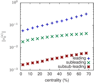
(a)  Centrality dependence of the (scaled) magnitudes of flows $\|v^{(a)}_{0}\|$.

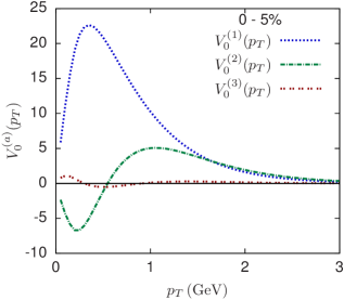
(b)  Momentum dependence of principal flow vectors $V_{0}^{(a)}(p_{T})$ in central collisions.

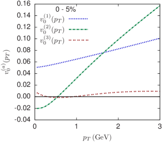
(c)  Principal flow vectors divided by the average multiplicity, $v_{0}^{(a)}(p_{T})\equiv V_{0}^{(a)}(p_{T})/\left<dN/dp_{T}\right>$.

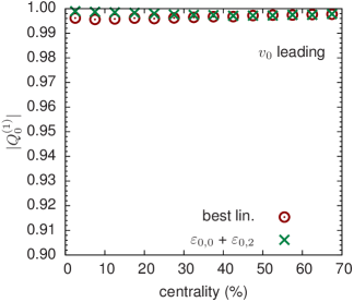
(d)  Pearson correlation coefficient between the leading flow (zero suppressed for clarity) and several predictors.

(e)  Pearson correlation coefficient between the subleading flow and several predictors.

Figure 9: $n=0$

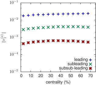
(a)  Centrality dependence of the (scaled) magnitudes of flows $\|v^{(a)}_{1}\|$.

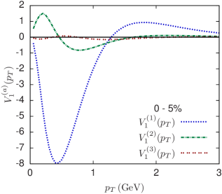
(b)  Momentum dependence of principal flow vectors $V_{1}^{(a)}(p_{T})$ in central collisions.

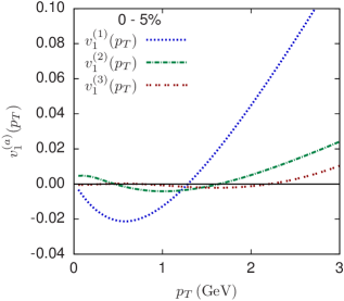
(c)  Principal flow vectors divided by the average multiplicity, $v_{1}^{(a)}(p_{T})\equiv V_{1}^{(a)}(p_{T})/\left<dN/dp_{T}\right>$.

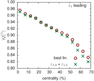
(d)  Pearson correlation coefficient between the leading flow (zero suppressed for clarity) and several predictors.

(e)  Pearson correlation coefficient between the subleading flow and several predictors.

Figure 10: $n=1$

(a)  Centrality dependence of the (scaled) magnitudes of flows $\|v^{(a)}_{2}\|$.

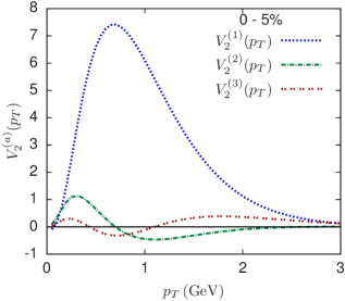
(b)  Momentum dependence of principal flow vectors $V_{2}^{(a)}(p_{T})$ in central collisions.

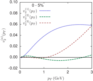
(c)  Principal flow vectors divided by the average multiplicity, $v_{2}^{(a)}(p_{T})\equiv V_{2}^{(a)}(p_{T})/\left<dN/dp_{T}\right>$.

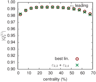
(d)  Pearson correlation coefficient between the leading flow (zero suppressed for clarity) and several predictors.

(e)  Pearson correlation coefficient between the subleading flow and several predictors.

Figure 11: $n=2$

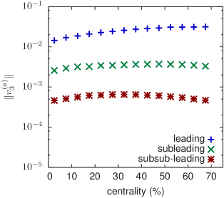
(a)  Centrality dependence of the (scaled) magnitudes of flows $\|v^{(a)}_{3}\|$.

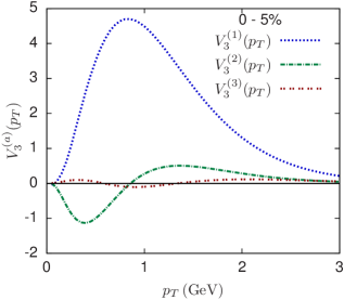
(b)  Momentum dependence of principal flow vectors $V_{3}^{(a)}(p_{T})$ in central collisions.

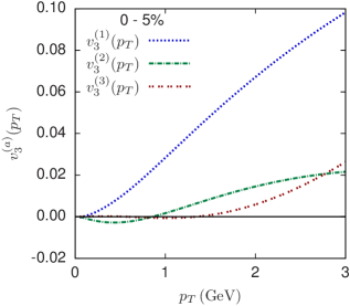
(c)  Principal flow vectors divided by the average multiplicity, $v_{3}^{(a)}(p_{T})\equiv V_{3}^{(a)}(p_{T})/\left<dN/dp_{T}\right>$.

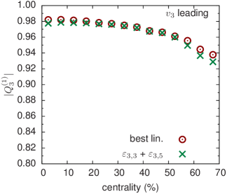
(d)  Pearson correlation coefficient between the leading flow (zero suppressed for clarity) and several predictors.

(e)  Pearson correlation coefficient between the subleading flow and several predictors.

Figure 12: $n=3$

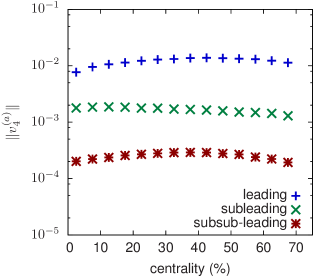
(a)  Centrality dependence of the (scaled) magnitudes of flows $\|v^{(a)}_{4}\|$.

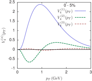
(b)  Momentum dependence of principal flow vectors $V_{4}^{(a)}(p_{T})$ in central collisions.

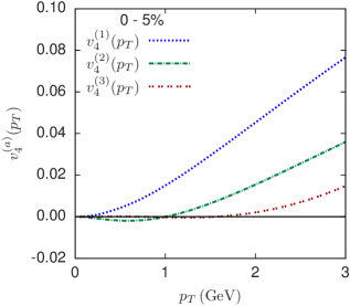
(c)  Principal flow vectors divided by the average multiplicity, $v_{4}^{(a)}(p_{T})\equiv V_{4}^{(a)}(p_{T})/\left<dN/dp_{T}\right>$.

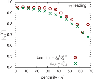
(d)  Pearson correlation coefficient between the leading flow (zero suppressed for clarity) and several predictors.

(e)  Pearson correlation coefficient between the subleading flow and several predictors.

Figure 13: $n=4$

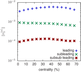
(a)  Centrality dependence of the (scaled) magnitudes of flows $\|v^{(a)}_{5}\|$.

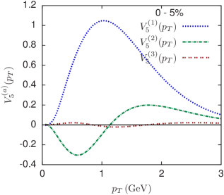
(b)  Momentum dependence of principal flow vectors $V_{5}^{(a)}(p_{T})$ in central collisions.

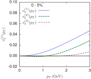
(c)  Principal flow vectors divided by the average multiplicity, $v_{5}^{(a)}(p_{T})\equiv V_{5}^{(a)}(p_{T})/\left<dN/dp_{T}\right>$.

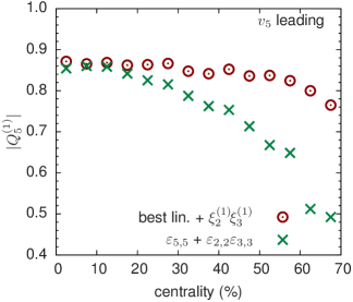
(d)  Pearson correlation coefficient between the leading flow (zero suppressed for clarity) and several predictors.

(e)  Pearson correlation coefficient between the subleading flow and several predictors.

Figure 14: $n=5$