Errors, correlations and fidelity for noisy Hamilton flows. Theory and numerical examples.

Abstract

We analyse the asymptotic growth of the error for Hamiltonian flows due to small random perturbations. We compare the forward error with the reversibility error, showing their equivalence for linear flows on a compact phase space. The forward error, given by the root mean square deviation $\sigma(t)$ of the noisy flow, grows according to a power law if the system is integrable and according to an exponential law if it is chaotic. The autocorrelation and the fidelity, defined as the correlation of the perturbed flow with respect to the unperturbed one, exhibit an exponential decay as $\exp\left({{-\sigma^{2}(t)}}\right)$. Some numerical examples such as the anharmonic oscillator and the Hénon Heiles model confirm these results. We finally consider the effect of the observational noise on an integrable system, and show that the decay of correlations can only be observed after a sequence of measurements and that the multiplicative noise is more effective if the delay between two measurements is large.

Keywords: Noisy Hamiltonian flow, Fidelity, Reversibility error, Observational noise.

1 Introduction

The Hamiltonian description of geophysical fluids has been extensively developed [1, 2, 3, 4] and is suited to analyse the conservation laws and to investigate approximation schemes which preserve the geometric invariants. These methods are also applicable to the Poisson-Vlasov equations for a collisionless plasma [5, 6]. Examples of Hamiltonian models of geophysical fluids are the canonical formulation of Rossby waves in a rotating sphere and the system of $N$ vortices.

Finite dimensional Hamiltonian systems are well understood in the integrable and uniformly hyperbolic limits, which correspond to an ordered quasiperiodic and a chaotic evolution [7]. The effect of small perturbations is amenable to analytical treatment in both situations, but the case of large perturbations and the transition from regular to chaotic regimes can only be explored numerically. In addition the effect of a weak noise and of round off errors in numerical computations deserves a special attention. The divergence of orbits and the memory loss rate of a given system are intimately related and reflect its dynamic behaviour. The Lyapunov exponents, and related indicators, specify the asymptotic separation rate of two initially close orbits [8], whereas the autocorrelation decay measures how fast the evolution loses its memory of a given initial condition. The asymptotic divergence of nearby orbits, the decay of correlations and the spectrum of Poincaré recurrences are intimately related. In particular the correlation decay rate is related to the Lyapunov spectrum [9].

When a small deterministic or stochastic perturbation is introduced into the system, the perturbed orbit diverges from the unperturbed one (with the same initial condition) and we call forward error (FE) their distance at time $t$ or the root mean square deviation at time $t$, if the perturbation is stochastic. The reversibility error (RE) is the distance, or the root mean square deviation, from the initial point, of its image after the evolution forward and backward for the same time interval $t$. The loss of memory with respect to the reference orbit is given, for instance, by the classical fidelity [10], first introduced in quantum systems [11].

For linear symplectic maps the asymptotic equivalence or RE and FE was proved in [12] and a relation with the fidelity decay was established. The fidelity behaviour for maps on the torus and the cylinder with random perturbations was first analysed in [13] and compared with the perturbation induced by round off errors [14, 15]. The RE analysis was first introduced to investigate the global effects of round off errors in symplectic maps in [16].

In this note we examine the asymptotic behaviour of FE and RE for Hamiltonian flows with a small random perturbation. In the case of linear flows we recover, with simpler proofs, the results previously obtained for linear symplectic maps. If the phase space is a compact set such as the torus ${\mathbb{T}}^{2d}$ then the autocorrelation and fidelity can be computed and their decay rate is related to the growth of the forward and reversibility errors.

Denoting with $\sigma(t)$ the FE and RE for a random perturbation, the asymptotic decay of fidelity is given by $F(t)\sim e^{-2\pi^{2}\,\sigma^{2}(t)}$. For an integrable system defined on the cylinder we prove that the error growth follows a power law $\sigma(t)\sim\epsilon t^{\beta}$ where $\beta=3/2$ if the system is anisochronous, $\beta=1/2$ if it is isochronous. The exponent $3/2$ is due to the conditional mixing, known as filamentation in the case of a rotating fluid. This kind of mixing is also responsible for the algebraic decay of the spectrum of Poincaré recurrences [17]. These results easily extend to integrable systems of higher dimension. If the unperturbed system is not skew the result very likely still holds, as suggested by numerical computations, though the proof is no longer elementary.

The proposed method could be applied to any finite dimensional dynamical system with a small additive noise because it is based on the linear equation satisfied by the Gaussian stochastic process which defines the forward and reversibility errors. Infinite dimensional extensions might be considered since the stochastic process satisfies a linear partial differential equation.

We have analysed numerically the behaviour of the anharmonic oscillator, the Hénon Heiles model, and a system of point vortices [18, 19, 20, 21]. The results obtained for these models agree with the ones previously obtained for the standard map and the three body system [12, 15]. Except for the vortex model the Hamiltonian reads $H=T(p)+V(q,t)-\epsilon\,x\,\xi(t)$ where $\xi(t)$ is a white noise and a symplectic integrator was used, 4-th order accurate for the deterministic component, just as for the three body problem. For a discussion on numerical stochastic integration see [22]. In the integrable and chaotic regions the results proved for linear systems are confirmed. In the transition regions the results might be interpreted following the model proposed for Poincaré recurrences [17].

Random perturbations are introduced by the environment and by observations: the effect of observational noise in dynamical systems is actively investigated, see [23, 24] and references therein. When the system is integrable the effect of a single observation is small. However a sequence of observations may cause an exponential decrease of the correlations or the fidelity. The multiplicative noise changes the signal in a way dependent on the signal itself and may determine a faster decay of fidelity when the change of phase between two observations is large.

2 Dynamical systems with additive noise

In a previous paper we have considered prototype model maps defined on the torus or the cylinder, whose invariant measure is the normalized Lebesgue measure. We consider first a 1D dynamical system with a stochastic perturbation defined by the Langevin equation

$${dx\over dt}=\Phi(x)+\epsilon\xi(t)$$

where $x\in{\mathbb{R}}$ and $\xi(t)$ is a white noise. We denote by $\langle\,\,\,\rangle$ average with respect to all the realizations of the stochastic process

$$\langle\xi(t)\rangle=0\qquad\qquad\langle\xi(t)\xi(t^{\prime})\rangle=\delta(t-t^{\prime})$$

We denote the deterministic solution with initial point $x_{0}$ with $x=S_{t}(x_{0})$ and with $f(x,t)$ the distribution function at time $t$ corresponding to an initial value $f(x_{0},0)=f(x_{0})$. The distribution function $f$ for the deterministic system satisfies the continuity equation

$${\partial{}\over\partial{t}}f(x,t)+{\partial{}\over\partial{x}}(\Phi(x)f(x,t))=0$$

The fundamental solution of the continuity equation is given by

$$G(x,x_{0};t)=\delta(x-S_{t}(x_{0}))={\delta(x_{0}-S_{-t}(x))\over\eta(S_{-t}(x),t)}\qquad\qquad\eta(x_{0},t)={\partial{S_{t}(x_{0})}\over\partial{x_{0}}}$$

since the solution $x=S_{t}(x_{0})$ is assumed to have a unique inverse $x_{0}=S_{-t}(x)$. The solution for the distribution function $f(x,t)$ corresponding to an initial distribution $f(x_{0},0)=f(x_{0})$ reads

$$f(x,t)=\int_{-\infty}^{+\infty}\,G(x,x_{0};t)\,f(x_{0})\,dx_{0}={f(S_{-t}(x))\over\eta(S_{-t}(x),t)}$$

When the noise is present we can still write a stochastic continuity equation given by (3) where $\Phi$ is replaced by $\Phi(x)+\epsilon\xi(t)$. In this case after averaging over the noise the distribution function satisfies the Fokker-Planck equation (see [10]).

$${\partial{}\over\partial{t}}f(x,t)+{\partial{}\over\partial{x}}(\Phi(x)f(x,t))={\epsilon^{2}\over 2}{\partial^{2}\over\partial x^{2}}\,f(x,t)$$

whose solution is given by

$$f_{\epsilon}(x,t)=\int_{-\infty}^{+\infty}\,G_{\epsilon}(x,x_{0};t)\,f(x_{0})\,dx_{0}$$

We denote with $G_{\epsilon}(x,x_{0};t)$ the fundamental solution of the Fokker-Planck equation, namely its solution with initial condition $G_{\epsilon}(x,x_{0};0)=\delta(x-x_{0})$. In the limit $\epsilon\to 0$ we recover the fundamental solution of equation (3). We write the solution of the Langevin equation as $x(t)=S_{\epsilon,\,t}(x_{0})$ where

$$S_{\epsilon,\,t}(x_{0})=S_{t}(x_{0})+\epsilon\chi(t)=S_{t}(x_{0})+\epsilon\Xi(t)+O(\epsilon^{2})$$

The stochastic process $\Xi(t)$ is the limit of $\chi(t)$ for $\epsilon\to 0$ and proves to be Gaussian since it satisfies the linearised equation

$${d\,\Xi\over dt}+{\mathsf{M}}(t)\,\Xi=\xi(t)\qquad\qquad{\mathsf{M}}(t)=\Phi^{\prime}(S_{t}(x_{0}))$$

Indeed $\Xi(t)$ can be written as a convolution of the white noise $\Xi(t)=\int_{0}^{t}\,K(t,s)\,\xi(s)\,ds$. If $\Phi(x)$ is linear

$$\Phi(x)=\omega+\beta x$$

then $\chi(t)$ and $\Xi(t)$ are equal. In this case the deterministic component is

$$S_{t}(x_{0})=e^{\beta t}\,x_{0}+\phi(t)\qquad\qquad\phi(t)=\omega\,\,{e^{\beta t}-1\over\beta}$$

and the fluctuating component is defined by

$$\chi(t)=\int_{0}^{t}\,\,e^{\beta(t-s)}\,\,\xi(s)ds\qquad\qquad\sigma^{2}(t)=\,\epsilon^{2}\,{e^{2\beta t}-1\over 2\beta}$$

As a consequence the fundamental solution of the Fokker-Planck equation (6) reads

$$G_{\epsilon}(x,t)={\exp\left({{-{\bigl{(}\displaystyle x-\langle x\rangle\bigr{)}^{2}\over\displaystyle 2\sigma^{2}(t)}}}\right)\over\sqrt{2\pi\sigma^{2}(t)}}\qquad\qquad\langle x(t)\rangle=S_{t}(x_{0})=e^{\beta t}x_{0}+\phi(t)$$

We notice that for $\epsilon=0$ the fundamental solution of the Fokker-Planck reduces to $\delta(x-S_{t}(x_{0}))$, namely the fundamental solution of the deterministic continuity equation (3). We remark also that the root mean square deviation for $\beta>0$ has an exponential growth $\sigma(t)\sim\epsilon e^{\beta t}$. If $\beta=0$ the motion becomes a translation and in this case $\sigma(t)=\epsilon\,t^{1/2}$.

3 Observables on the torus and correlations

In order to have a chaotic behaviour an exponential divergence of the flow and the phase space compactness are required. This can be achieved by considering a dynamical system on the torus ${\mathbb{T}}$. The torus can be seen as the interval $[0,1]$, where the endpoints are identified. Any periodic function of period 1 defined on ${\mathbb{R}}$ is a dynamic variable on ${\mathbb{T}}^{1}$. If $f(x)$ is any function defined on ${\mathbb{R}}$ we may construct a dynamic variable $f_{\mathbb{T}}(x)$ in the following way

$$f_{\mathbb{T}}(x)=\sum_{j=-\infty}^{+\infty}\,\,f(x+j)$$

provided that the decrease of $f(x)$ at infinity is sufficiently fast to insure the convergence of the series. The function $f_{\mathbb{T}}(x)$ is periodic of period 1 by construction and therefore can be expanded in a Fourier series

$$f_{\mathbb{T}}(x)=\sum_{k=-\infty}^{+\infty}\,\,\hat{f}_{k}\,e^{2\pi\,i\,k\,x}$$

whose coefficients are given by

$$\eqalign{\hat{f}_{k}&=\int_{0}^{1}\,e^{-2\pi\,i\,k\,x}\,f_{\mathbb{T}}(x)\,dx=\sum_{j=-\infty}^{+\infty}\,\int_{0}^{1}\,\,e^{-2\pi\,i\,k\,x}\,f(x+j)\,dx\cr&\cr&=\sum_{j=-\infty}^{+\infty}\,\int_{j}^{j+1}\,\,e^{-2\pi\,i\,k\,(x-j)}\,f(x)\,dx=\int_{-\infty}^{+\infty}\,\,e^{-2\pi\,i\,k\,x}\,f(x)\,dx\cr}$$

If $f(x)\in L^{1}({\mathbb{R}})$ its Fourier transform $\hat{f}(k)$ for $k\in{\mathbb{R}}$ is defined by

$$\hat{f}(k)=\int_{-\infty}^{+\infty}\,\,e^{-2\pi\,i\,k\,x}\,f(x)\,dx$$

and consequently $\hat{f}_{k}=\hat{f}(k)$ for $k\in{\mathbb{Z}}$.

If $f(x,t)$ is the solution of the continuity equation on ${\mathbb{R}}$ the corresponding solution on ${\mathbb{T}}$ is given by

$$\eqalign{f_{\mathbb{T}}(x,t)=\sum_{j=-\infty}^{+\infty}\,\,f(x+j,t)=&\sum_{j=-\infty}^{+\infty}\,\,\int_{-\infty}^{+\infty}\delta(x+j-S_{t}(x_{0}))\,f(x_{0})\,dx_{0}=\cr&\cr&=\,\int_{-\infty}^{+\infty}\,G_{\mathbb{T}}(x,x_{0},t)\,f(x_{0})\,dx_{0}\cr}$$

By $G_{\mathbb{T}}(x,x_{0},t)$ we denote the fundamental solution on ${\mathbb{T}}^{1}$ whose Fourier expansion is given by

$$G_{\mathbb{T}}(x,x_{0};t)=\sum_{j=-\infty}^{+\infty}\,\delta(x+j-S_{t}(x_{0}))\,=\sum_{k=-\infty}^{+\infty}\,\,e^{2\pi\,i\,kx}\,e^{-2\pi\,i\,k\,\,S_{t}(x_{0})}$$

By replacing (18) into (17) we obtain the Fourier expansion of $f_{\mathbb{T}}(x,t)$ according to

$$f_{\mathbb{T}}(x,t)=\sum_{k=-\infty}^{+\infty}\,\,\hat{f}_{k}(t)\,e^{2\pi\,i\,k\,x}\,\qquad\qquad\hat{f}_{k}(t)=\int_{-\infty}^{+\infty}\,dx_{0}\,e^{-2\pi\,i\,k\,S_{t}(x_{0})}\,f(x_{0})$$

We introduce also the following coefficients

$$f_{k}(t)=\int_{0}^{1}\,dx_{0}\,e^{-2\pi\,i\,k\,S_{t}(x_{0})}\,f_{\mathbb{T}}(x_{0})$$

Notice that for $t=0$ we have $\hat{f}_{k}(0)=\hat{f}_{k}$. The new time dependent coefficients differ from the Fourier components unless the evolution is just a translation $S_{t}(x)=x_{0}+\omega t$ or $f(x)$ has support on $[0,1]$ vanishing elsewhere. In this case

$$f_{k}(t)=\hat{f}_{k}(t)$$

and the following equality holds

$$\int_{0}^{1}f_{\mathbb{T}}(x)\,f_{\mathbb{T}}(x,t)\,dx=\int_{0}^{1}\,f_{\mathbb{T}}(x_{0})\,f_{\mathbb{T}}(S_{t}(x_{0}))\,dx_{0}$$

3.1 Correlations

We introduce two distinct definitions of the correlation on the torus according to

$$\hat{C}(t)=\int_{0}^{1}\,f_{\mathbb{T}}(x)\,f_{\mathbb{T}}(x,t))\,dx-f_{0}^{2}=\sum_{k\not=0}\,\hat{f}_{-k}\hat{f}_{k}(t)$$

see equation (19)

$$C(t)=\int_{0}^{1}\,f_{\mathbb{T}}(x_{0})\,f_{\mathbb{T}}(S_{t}(x_{0}))\,dx_{0}-f_{0}^{2}=\sum_{k\not=0}\,\hat{f}_{-k}f_{k}(t)$$

see equation (20). These definitions are equivalent when $S_{t}$ is a translation or $f(x)$ has support on $[0,1]$. In general we can write $C(t)$ according to

$$C(t)=\sum_{(k^{\prime},k)\not=(0,0)}\hat{f}_{k^{\prime}}\,A_{k^{\prime},-k}\,\hat{f}_{-k}\qquad\qquad A_{k^{\prime},-k}=\int_{0}^{1}\,dx_{0}\,\,e^{2\pi\,i(k^{\prime}\,x_{0}-k\,S_{t}(x_{0})\,)}$$

When the vector field $\Phi(x)$ is linear, see equation (9), and the flow is linear, see equation (10), then $C(t)=\hat{C}(t)$ for a sequence of times $t=t_{m}$ where $t_{m}=\beta^{-1}\,\log m$ for $m\in{\mathbb{Z}}$. Indeed from equations (19), (10) and (16) we have

$$\hat{f}_{k}(t)=e^{-2\pi\,i\,k\,\phi(t)}\,\hat{f}(ke^{\beta t})$$

The coefficients $f_{k}(t)$, according to equations (23) and (24), are given by

$$f_{k}(t)=\sum_{k^{\prime}=-\infty}^{+\infty}\,\hat{f}_{k^{\prime}}\,A_{k^{\prime},-k}\,$$

where $A_{k^{\prime},-k}$ is given by

$$A_{k^{\prime},-k}=e^{-2\pi\,i\,k\phi(t)}\,\cases{e^{\pi i(k^{\prime}-k\,e^{\beta t})}\sin(\pi(k^{\prime}-ke^{\beta t})/(\pi(k^{\prime}-k\,e^{\beta t}))&if $e^{\beta t}\not=m$\cr&\cr\delta_{k^{\prime},mk}&if $e^{\beta t}=m$\cr}$$

As a consequence, for $t=t_{m}$, from (26) and (27) we have

$$f_{k}(t_{m})=\hat{f}_{k}(t_{m})=e^{-2\pi\,i\,k\phi(t_{m})}\hat{f}_{km}=e^{-2\pi\,i\,k\phi(t_{m})}\hat{f}_{ke^{\beta t_{m}}}$$

4 Noisy systems on the torus: correlations and fidelity

For a noisy system the evolution of a given initial distribution is given by equation (7) and if the system is defined on the torus ${\mathbb{T}}$ the evolution of the corresponding distribution $f_{\mathbb{T}}(x)$ defined by (13) is a periodic function in $x$ which can be expanded in a Fourier series according to

$$f_{\epsilon,\,{\mathbb{T}}}(x,t)=\int_{-\infty}^{+\infty}\,G_{\epsilon\,{\mathbb{T}}}(x,x_{0};t)\,f_{0}(x_{0})\,dx_{0}=\sum_{k=-\infty}^{+\infty}\,\hat{f}_{\epsilon,\,k}(t)\,e^{2\pi\,i\,kx}$$

where $G_{\epsilon\,{\mathbb{T}}}(x,x_{0};t)$ denotes the fundamental solution of the Fokker-Planck equation on the torus and $f_{\mathbb{T}}(x,t)$ the distribution function on the torus at time $t$

$$G_{\epsilon\,{\mathbb{T}}}(x,x_{0};t)=\sum_{j=-\infty}^{+\infty}\,\,G_{\epsilon}(x+j,x_{0};t)\qquad\qquad f_{\epsilon,\,{\mathbb{T}}}(x,t)=\sum_{j=-\infty}^{+\infty}f_{\epsilon}(x+j,t)$$

Even in this case we introduce two distinct definitions of correlations as an obvious extension of the noiseless case

$$\hat{C}_{\epsilon}(t)=\int_{0}^{1}\,f_{\mathbb{T}}(x)\,f_{\epsilon,\,{\mathbb{T}}}(x,t)\,dx-f_{0}^{2}=\sum_{k\not=0}\,\hat{f}_{-k}\,\hat{f}_{\epsilon,\,k}(t)$$

and

$$C_{\epsilon}(t)=\int_{0}^{1}\,f_{\mathbb{T}}(x_{0})\,\langle f_{{\mathbb{T}}}\bigl{(}\,S_{\epsilon,\,t}(x_{0})\,\bigr{)}\rangle\,dx_{0}-f_{0}^{2}=\sum_{k\not=0}\,\hat{f}_{-k}\,f_{\epsilon,\,k}(t)$$

where

$$f_{\epsilon,k}(t)=\int_{0}^{1}\,\langle e^{-2\pi\,i\,k\,S_{\epsilon,t}(x_{0})}\rangle\,f_{\mathbb{T}}(x_{0})\,dx_{0}$$

The fidelity gives the correlation between a dynamic variable $f(x)$ evaluated along the perturbed orbit at time $t$ and $f(x)$ evaluated along the unperturbed orbit at the same time. We have a unique definition of fidelity given by

$$\eqalign{F_{\epsilon}(t)&=\int_{0}^{1}\,f_{\mathbb{T}}(S_{t}(x_{0}))\,\langle f_{{\mathbb{T}}}\bigl{(}\,S_{\epsilon,\,t}(x_{0})\,\bigr{)}\rangle\,dx_{0}-f_{0}^{2}=\cr&=\sum_{(k,k^{\prime})\not=(0,0)}\,\hat{f}_{-k}\hat{f}_{k^{\prime}}\,\,\int_{0}^{1}\,dx_{0}\langle e^{2\pi\,i\,(k^{\prime}\,S_{\epsilon,\,t}(x_{0})-kS_{t}(x_{0})}\rangle}$$

4.1 Linear systems

For a linear Langevin equation, namely for $\Phi(x)=\beta x+\omega$, explicit expressions can be obtained. Indeed, to evaluate $\hat{f}_{\epsilon,\,k}(t)$, we expand $G_{\epsilon\,{\mathbb{T}}}(x,x_{0};t)$ in Fourier series, taking (8) and (11) into account. The result is

$$\eqalign{G_{\epsilon,\,k}(x_{0},\,t)=\int_{0}^{1}\,dx\,e^{-2\pi\,i\,kx}\,\,G_{\epsilon\,{\mathbb{T}}}(x,x_{0};t)&=\int_{-\infty}^{+\infty}\,e^{-2\pi\,i\,kx}\,{\exp\left({{-{\bigl{(}\displaystyle x-S_{t}(x_{0})\bigr{)}^{2}\over\displaystyle 2\sigma^{2}(t)}}}\right)\over\sqrt{2\pi\sigma^{2}(t)}}\cr&\cr&=e^{-2\pi ik\,S_{t}(x_{0})}\,e^{-2\pi^{2}\,\sigma^{2}(t)}\cr}$$

The Fourier components of $f_{\epsilon\,{\mathbb{T}}}(x,t)$ are given by

$$\hat{f}_{\epsilon,\,k}(t)=e^{-2\pi^{2}\,\sigma^{2}(t)}\,\,\int_{-\infty}^{+\infty}\,\,e^{-2\pi ik\,S_{t}(x_{0})}\,f(x_{0})\,dx_{0}=e^{-2\pi^{2}\,\sigma^{2}(t)}\,\,\hat{f}_{k}(t)$$

In order to evaluate $f_{\epsilon,\,k}(t)$ we recall that for a linear Langevin equation (1) where $\Phi(x)$ is given by (9) the solution $S_{\epsilon,\,t}(x_{0})$ is given by (8) and (11) so that

$$\langle e^{-2\pi\,i\,kS_{\epsilon,\,t}(x_{0})}\rangle=e^{-2\pi\,i\,k\,S_{t}(x_{0})}\langle e^{-2\pi\,i\,k\,\epsilon{\chi(t)}}\rangle=e^{-2\pi\,i\,k\,S_{t}(x_{0})}\,e^{-2\pi^{2}k^{2}\sigma^{2}}$$

As a consequence taking equation (16) into account we can write

$$f_{\epsilon,\,k}(t)=e^{-2\pi^{2}k^{2}\sigma^{2}}f_{k}(t)$$

The explicit expression for the correlation is

$$\hat{C}_{\epsilon}(t)=\sum_{k\not=0}\,\hat{f}_{-k}\,\hat{f}_{\,k}(t)\,e^{-2\pi^{2}k^{2}\sigma^{2}(t)}$$

and

$$C_{\epsilon}(t)=\sum_{(k,k^{\prime})\not=(0,0)}\,\hat{f}_{k^{\prime}}\,A_{k^{\prime},-k}\,\hat{f}_{-k}\,,e^{-2\pi^{2}\,k^{2}\,\sigma^{2}(t)}$$

In this case the fidelity has the following expression

$$F_{\epsilon}(t)=\sum_{(k,k^{\prime})\not=(0,0)}\,\hat{f}_{-k}\,\hat{f}_{k^{\prime}}\,\int_{0}^{1}\,dx_{0}\,e^{2\pi\,i\,(k^{\prime}-k)\,S_{t}x_{0}}\,\,\,\,\,e^{-2\pi^{2}\sigma^{2}(t)}$$

5 Model systems

We consider first three different prototype models

i) Translations on the torus ${\mathbb{T}}^{1}$.

The field is $\Phi(x)=\omega$ and $S_{t}(x_{0})=x_{0}+\omega t$ and the Fourier coefficients are

$$f_{k}(t)=\hat{f}_{k}(t)=e^{-2\pi\,i\,k\,\omega t}\,\hat{f}_{k}$$

The correlations do not decay.

When the noise is introduced the root mean square deviation with respect to the unperturbed trajectory is $\sigma=\epsilon\,t^{1/2}$ and the Fourier coefficients are given by

$$f_{\epsilon\,k}(t)=\hat{f}_{\epsilon\,k}(t)=e^{-2\pi\,i\,k\,\omega t}\,\hat{f}_{k}\,e^{-2\pi^{2}\epsilon^{2}t}$$

The decay of correlations and fidelity is exponential with decay time $\tau=(2\pi^{2}\epsilon^{2})^{-1}$. The difference is that the correlations oscillate and decay, while the fidelity goes to zero without oscillations, due to the absence of the phase factor.

ii) Anisochronous translations on the cylinder

This is a skew system. Letting ${\mathbf{x}}=(x,y)\in{\mathbb{C}}={\mathbb{T}}\times{\mathbb{I}}$ be the phase space coordinates, ${\mathbf{\Phi}}=(y,0)$ the vector field and $S_{t}({\mathbf{x}}_{0})=(x_{0}+y_{0}t,y_{0})$ the flow, for an observable $f(x)$ to which corresponds $f_{\mathbb{T}}(x)$ on the torus we have

$$\hat{f}_{k}(t)=f_{k}(t)=e^{-i\,k\,y_{0}t}\,\hat{f}_{k}$$

Even though $f_{\mathbb{T}}$ does not depend on the torus label $y_{0}$ the coefficient $f_{k}(t)$ depend on it according to the previous equation. The correlation is computed by averaging on the interval ${\mathbb{I}}=[0,a]$ to which $y_{0}$ belongs. Taking account of the normalization factor $a^{-1}$ the correlation reads

$$C(t)=\hat{C}(t)=\sum_{k\not=0}\,|f_{k}|^{2}\,{1\over a}\,\int_{0}^{a}\,e^{-2\pi\,i\,k\,y_{0}\,t}\,dy_{0}=\sum_{k\not=0}\,|f_{k}|^{2}\,\ e^{-\pi\,i\,k\,a\,t}\,\,{\sin(\pi\,k\,a\,t)\over\pi\,k\,a\,t}$$

as a consequence supposing that $|f_{k}|<A/|k|$ we have

$$|C(t)|<{3A^{2}\over\pi a}\,{1\over t}$$

and the decay follows a power law. This slow decay is due to the conditional mixing, known in physics as the filamentation phenomenon, which occurs because the frequency on the tori has a continuous and monotonic variation. For an observable $f(x,y)$ such that the average on $x$ is constant, the result still holds provided that the Fourier coefficients $\hat{f}_{k}(y)$ are $C^{1}$ and decay faster than $1/y$ at infinity.

Any autonomous 1D system in the region around a stable fixed point delimited by the separatrices is defined, using action angle variables $(\phi,\jmath)$, by the vector field ${\mathbf{\Phi}}=(\omega(j),0)$. If $\omega(j)$ is monotonic, introducing the new variables $x=\phi/(2\pi)$ and $y=\omega(\jmath)$ we are back to the case considered above.

When a stochastic perturbation is introduced the vector field becomes ${\mathbf{\Phi}}(x,y)=\bigl{(}\,y+\epsilon\xi_{x}(t),\epsilon\xi_{y}(t)\,\bigr{)}$ where $\xi_{x}(y)$ and $\xi_{y}(t)$ are two independent white noises. In this case the stochastic flow $S_{\epsilon,\,t}(x_{0},y_{0})$ is given by

$$x=x_{0}+y_{0}t\,+\epsilon w_{y}^{(1)}(t)+\epsilon w_{x}(t)\qquad\qquad y=y_{0}+\epsilon w_{y}(t)$$

where $w(t)=\int_{0}^{t}\,\xi(s)\,ds$ denotes a Wiener noise and $w^{(1)}(t)=\int_{0}^{t}\,w(s)\,ds$. Recalling that $\langle w_{x}^{2}(t)\rangle=t$, $\langle(w_{y}^{(1)}(t))^{2}\rangle=t^{3}/3$, $\langle w_{x}(t)w_{y}^{(1)}(t)\rangle=0$, the root mean square deviations for $x$ and $y$ are given by

$$\sigma_{x}=\epsilon\left({{t+{t^{3}\over 3}}}\right)^{1/2}\qquad\qquad\sigma_{y}=\epsilon\,t^{1/2}$$

The correlation on the cylinder for the observable $f_{\mathbb{T}}(x)$ is given by

$$C(t)=\sum_{k\not=0}|f_{k}|^{2}\,\left[{{e^{-\pi\,i\,k\,a\,t}\,\,{\sin(\pi\,k\,a\,t)\over\pi\,k\,a\,t}}}\right]\,e^{-2\pi^{2}\,k\,\epsilon^{2}(t+t^{3}/3)}$$

The fidelity has the same expression where the term within the square parenthesis is replaced by 1. If the frequency is the same on each torus, or if the $y$ variable is not affected by noise, the decay of correlations or fidelity is much slower since the cubic term in the exponential is absent.

iii) Expanding flow

Given the vector field $\Phi(x)=\beta x$, the flow is $S_{t}(x_{0})=e^{\beta t}x_{0}$ and the Fourier coefficients are given by

$$\hat{f}_{k}(t)=\int_{-\infty}^{+\infty}\,f(x)\,e^{2\pi\,i\,k\,x_{0}e^{\beta t}}=\hat{f}(k\,e^{\beta t})$$

If $f(x)\in L^{2}$ then $\hat{f}(k)\in L^{2}$ and consequently $|\hat{f}(k)|$ decreases to $0$ for $|k|\to\infty$. If $|\hat{f}_{k}|\leq A\,|k|^{-1}$ then $\hat{f}(ke^{\beta t})$ decreases exponentially fast to zero with $t$ and the following estimate holds

$$|\hat{C}(t)|\leq 2A^{2}\,e^{-\beta t}\,\sum_{k=1}^{\infty}\,{1\over k^{3}}\leq 3A^{2}\,e^{-\beta t}$$

The Fourier coefficients entering the other definition of correlation are, for $e^{\beta t}\not\in{\mathbb{N}}$,

$$f_{k}(t)=\int_{0}^{1}\,f_{\mathbb{T}}(x_{0})\,e^{-2\pi\,i\,k\,x_{0}e^{2\beta t}}\,dx_{0}=\sum_{k^{\prime}=-\infty}^{+\infty}\,f_{k^{\prime}}e^{+\pi\,i\,(k^{\prime}-ke^{\beta t})}\,{\sin\pi(k^{\prime}-ke^{\beta t})\over k^{\prime}-ke^{\beta t}}$$

If $e^{\beta t}=m\in{\mathbb{N}}$ then letting $t_{m}=\beta^{-1}\,\log m$ we have $\hat{f}_{k}(t_{m})=f_{k}(t_{m})=\hat{f}_{mk}$ where $|\hat{f}_{mk}|\leq\,e^{-\beta t_{m}}\,A/|k|$. If $f(x)$ has a compact support on $[0,1]$ the two definitions agree for any $t\in{\mathbb{R}}$.

When the noise is present the root mean square deviation is given by

$$\sigma=\left({{e^{2\beta t}-1\over 2\beta}}\right)^{1/2}$$

The correlations consequently are given by (38) and (39) , the fidelities by (40) where $\hat{f}_{k}(t)$ and $f_{k}(t)$ are given by equations (49) and (51) respectively.

The explicit expressions of correlations for $e^{\beta t}\not\in{\mathbb{N}}$ is

$$\hat{C}_{\epsilon}(t)=\sum_{k\not=0}\,\hat{f}_{-k}\,\hat{f}(ke^{\beta t})\,e^{-2\pi^{2}k^{2}\sigma^{2}(t)}$$

and

$$C_{\epsilon}(t)=\sum_{(k,k^{\prime})\not=(0,0)}\,f_{-k}\,f_{k^{\prime}}\,\,e^{\pi\,i\,(k^{\prime}-ke^{\beta t})}\,\,{\sin\pi((k^{\prime}-ke^{\beta t})\over\pi(k^{\prime}-ke^{\beta t})}\,e^{-2\pi^{2}k^{2}\sigma^{2}(t)}$$

The explicit expression for the fidelity reads

$$F_{\epsilon}(t)=\sum_{(k,k^{\prime})\not=(0,0)}\,f_{-k}\,f_{k^{\prime}}\,\,e^{\pi\,i\,(k^{\prime}-k)e^{\beta t}}\,\,{\sin\pi((k^{\prime}-k)e^{\beta t}\over\pi\,i(k^{\prime}-k)e^{\beta t}}\,\,e^{-2\pi^{2}k^{2}\,\sigma^{2}(t)}$$

For $e^{\beta t}=m\in{\mathbb{N}}$ we have

$$\hat{C}_{\epsilon}(t_{m})=C_{\epsilon}(t_{m})=\sum_{k\not=0}\,\hat{f}_{-k}\,\hat{f}_{mk}\,e^{-2\pi^{2}k^{2}\sigma^{2}(t_{m})}\qquad F_{\epsilon}(t_{m})=\sum_{k\not=0}\,|f_{k}|^{2}\,\,e^{-2\pi^{2}k^{2}\sigma^{2}(t_{m})}$$

6 Reversibility error and related fidelity

The reversibility error is the distance from the initial point of its forward evolution up to time $t$ and backward for the same time interval. Any autonomous flow is reversible since the flow $S_{t}$ has the group property $S_{-t}\circ S_{t}=I$. This property is lost when the system is stochastically perturbed. In this case the local errors $\epsilon\xi(\pm t)$ at times $\pm t$ are independent and we have $S_{\epsilon,-t}\circ S_{\epsilon,t}\not=I$.

We define a fidelity associated to the reversibility error according to

$$F_{\epsilon\,R}(t)=\int_{0}^{1}\,dx_{0}\,f_{\mathbb{T}}(x_{0})\,\langle f_{\mathbb{T}}(S_{\epsilon,-t}\circ S_{\epsilon,t}(x_{0}))\rangle-f_{0}^{2}$$

The FE and the RE are related, and for linear flows we prove they are equal up to a factor $\sqrt{2}$.

We consider first the translation perturbed with a white noise whose flow is $S_{\epsilon,\,t}\,x_{0}=x_{0}+\omega t+\epsilon w(t)$ so that $S_{\epsilon,\,-t}\circ S_{\epsilon,\,t}\,x_{0}=x_{0}+\epsilon(w(t)+w(-t))$. The reversibility error is given by the root mean square deviation of this process $\sigma_{R}(t)=\epsilon\sqrt{2}\,t^{1/2}$, since $\langle w(t)w(-t)\rangle=0$. If the flow is expanding, namely $\Phi_{\epsilon}=\beta x+\epsilon\xi(t)$ then we have

$$S_{\epsilon,\,-t}\circ S_{\epsilon,\,t}\,x_{0}=x_{0}+\epsilon\chi_{R}(t)\qquad\qquad\chi_{R}(t)=e^{-\beta t}\chi(t)+\chi(-t)$$

As a consequence from

$$\chi_{R}(t)=\int_{0}^{t}e^{-\beta s}\,(\xi(s)-\xi(s-t))ds$$

we obtain the reversibility error

$$\sigma_{R}(t)=\epsilon\langle\chi_{R}^{2}(t)\rangle^{1/2}=\epsilon\sqrt{2}\,{1-e^{-2\beta t}\over 2\beta}$$

The reversibility error $\sigma_{R}(t)$ is equal to the forward error $\sigma(t)$ (times $\sqrt{2}$) but for the system whose vector field is $\Phi(x)=-\beta x$ rather than $\Phi(x)=\beta x$. The forward flow is expanding, the reverse flow is contracting, but RE for the expanding flow is equal to the FE for the contracting flow. To recover the equivalence it is sufficient to consider the flow on the torus ${\mathbb{T}}^{2}$ defined by the following noisy vector field $\Phi_{\epsilon}=(-\beta x+\epsilon\xi_{x}(t),\beta y+\epsilon\xi_{y}(t))$ where $\xi_{t}(t)$ and $\xi_{y}(t)$ are independent white noises. A simple computation shows that in this case $\sigma_{R}(t)=\sqrt{2}\,\sigma(t)$. The deterministic flow in this case is area preserving. More generally linear Hamiltonian flows exhibit the same equivalence asymptotically.

6.1 Quadratic Hamiltonians

We consider the general case of a quadratic Hamiltonian $H({\mathbf{x}})={1\over 2}\,{\mathbf{x}}\cdot{\mathsf{B}}{\mathbf{x}}$ where ${\mathbf{x}}\in{\mathbb{R}}^{2d}$ for an arbitrary number of degrees of freedom $d$ and ${\mathsf{B}}$ is a symmetric matrix. The equations of motion and the flow are

$${d{\mathbf{x}}\over dt}={\mathsf{A}}\equiv{\mathsf{J}}{\mathsf{B}}\qquad\qquad{\mathsf{J}}=\pmatrix{0&I\cr-I&0\cr}\qquad\qquad S_{t}{\mathbf{x}}_{0}=e^{{\mathsf{A}}t}{\mathbf{x}}_{0}$$

where the matrix $e^{{\mathsf{A}}t}$ is symplectic namely $e^{t{\mathsf{A}}}{\mathsf{J}}\,e^{t{\mathsf{A}}^{T}}={\mathsf{J}}$. When the system is stochastically perturbed the equations of motion and the stochastic flow become

$${d{\mathbf{x}}\over dt}={\mathsf{A}}{\mathbf{x}}+\epsilon\,{\mathbf{\xi}}(t)\qquad\qquad S_{\epsilon,\,t}{\mathbf{x}}_{0}=e^{{\mathsf{A}}t}{\mathbf{x}}_{0}+\epsilon{\mathbf{\chi}}(t)\qquad\qquad{\mathbf{\chi}}(t)=\int_{0}^{t}e^{{\mathsf{A}}(t-s)}\,{\mathbf{\xi}}(s)\,ds$$

The RE is computed starting from the reversed flow

$$S_{\epsilon,\,-t}\,S_{\epsilon,\,t}\,{\mathbf{x}}_{0}={\mathbf{x}}_{0}+{\mathbf{\chi}}_{R}(t)\qquad\quad{\mathbf{\chi}}_{R}(t)=\epsilon\bigl{[}e^{-{\mathsf{A}}t}{\mathbf{\chi}}(t)+{\mathbf{\chi}}(-t)\bigr{]}=\int_{0}^{t}e^{-s{\mathsf{A}}}(\,{\mathbf{\xi}}(s)-{\mathbf{\xi}}(s-t))\,\,ds$$

and explicitly reads

$$\sigma^{2}_{R}(t)=\epsilon^{2}\,\left\langle\,\left\|{\mathbf{\chi}}_{R}(t)\right\|^{2}\,\,\right\rangle=2\epsilon^{2}\,\int_{0}^{t}\,ds\,\,\hbox{Tr}\,\left({{e^{-s\,{\mathsf{A}}}\,e^{-s\,{\mathsf{A}}^{T}}}}\right)$$

The forward error $\sigma(t)$ is defined by

$$\sigma^{2}(t)=\epsilon^{2}\,\left\langle\,\left\|\chi(t)\right\|^{2}\,\,\right\rangle=\epsilon^{2}\,\int_{0}^{t}\,ds\,\,\hbox{Tr}\,\left({{e^{s\,{\mathsf{A}}}\,e^{s\,{\mathsf{A}}^{T}}}}\right)$$

It is not hard to prove that $\sigma(t)$ and $\sigma_{R}(t)/\sqrt{2}$ are asymptotically equal taking into account the property of symplectic matrices. Indeed $e^{{\mathsf{A}}t}$ and $e^{-{\mathsf{A}}t}$ have the same eigenvalues.

The fidelity $F_{R}(t)$ for a noisy reversed flow on the torus ${\mathbb{T}}^{2d}$ is defined by

$$F_{R}(t)=\int_{0}^{1}\,d{\mathbf{x}}_{0}\,\,f_{{\mathbb{T}}^{2d}}\,({\mathbf{x}}_{0})\,\,f_{{\mathbb{T}}^{2d}}\,(S_{\epsilon,\,-t}S_{\epsilon,\,t}\,{\mathbf{x}}_{0})\,-\left({{\int_{0}^{1}\,d{\mathbf{x}}_{0}\,\,f_{{\mathbb{T}}^{2d}}({\mathbf{x}}_{0}}}\right)^{2}$$

The reversed flow is given by equation (62) where the global error $\epsilon\chi_{R}(t)$ is defined. Expanding $f_{{\mathbb{T}}^{2d}}({\mathbf{x}})$ in a Fourier series we find

$$\eqalign{F_{R}(t)=\sum_{({\mathbf{k}},{\mathbf{k}}^{\prime})\not=({\bf 0},{\bf 0})}\,f_{-{\mathbf{k}}}\,f_{{\mathbf{k}}^{\prime}}\,\,\int_{0}^{1}\,dx_{0\,1}\,\cdots&\int_{0}^{1}\,dx_{0\,2d}\,\,e^{-2\pi\,i\,({\mathbf{k}}^{\prime}-{\mathbf{k}})\cdot{\mathbf{x}}_{0}}\,\langle e^{2\pi\,i\,{\mathbf{k}}^{\prime}\,\epsilon\,{\mathbf{\chi}}_{R}(t)}\rangle=\cr&=\sum_{({\mathbf{k}},{\mathbf{k}}^{\prime})\not=({\bf 0},{\bf 0})}\,f_{-{\mathbf{k}}}\,f_{{\mathbf{k}}^{\prime}}\,e^{-4\pi^{2}\,{\mathbf{k}}\cdot\Sigma^{2}(t)\,{\mathbf{k}}}\cr}$$

where

$$\Sigma^{2}(t)=\epsilon^{2}\int_{0}^{t}ds\,\,e^{-{\mathsf{A}}s}\,e^{-{\mathsf{A}}^{T}s}$$

We recall that the square of the reversibility error is expressed by

$$\sigma_{R}^{2}(t)=\epsilon^{2}\,\,\hbox{Tr}\,\bigl{(}\Sigma^{2}(t)\bigr{)}$$

If all the eigenvalues are complex of unit modulus then $e^{s{\mathsf{A}}}$ is conjugated to an orthogonal matrix. If $e^{s{\mathsf{A}}}$ is orthogonal $\sigma^{2}(t)=2d\,\epsilon^{2}\,t$ supposing the phase space is ${\mathbb{R}}^{2d}$. If $A$ has real eigenvalues $\pm\lambda_{i}$ ordered in an increasing sequence $-\lambda,-\lambda_{2},\ldots,\lambda_{2},\lambda$ then $e^{tA}$ is conjugated to the diagonal matrix $e^{t\Lambda}=\hbox{diag}\,(e^{\lambda t},\,e^{\lambda_{2}\,t},\ldots,e^{-\lambda_{2}t},e^{-\lambda t})$. Supposing for simplicity that ${\mathsf{A}}=\Lambda$ is diagonal (in the general case only trivial constant factors appear) we obtain that asymptotically

$$\sigma(t)\simeq\epsilon e^{\lambda t}\qquad\qquad\sigma_{R}(t)\simeq\,\sqrt{2}\,\epsilon\,e^{\lambda t}\qquad\qquad{\mathbf{k}}\cdot\Sigma^{2}_{R}(t){\mathbf{k}}=k_{1}^{2}\,\epsilon^{2}\,e^{2\lambda t}$$

Also in this more general case the asymptotic decay rate of fidelity is related to the asymptotic growth of the error.

7 Models

We give some examples of application of the previous results. To this end we consider as integrable system the anharmonic oscillator and as non integrable system the Hénon Heiles Hamiltonian. The Hamilton’s equations are integrated by using symplectic 4-th order integrators, based on the splitting method. Finally we consider the system of vortices for which explicit symplectic integrators are not available: we use then a Runge-Kutta integrator. The restricted 3 body problem has been discussed elsewhere [12] just as native discrete systems expressed by symplectic maps [14].

Denoting the time step by $\Delta t=T/n_{s}$, where $T$ is a characteristic time of the system, and using fourth order methods, we insure that the local integration error is close to the round off choosing $n_{s}=10^{4}$. In addition symplectic integrators insure that the error on the invariants has a null average growth. We consider also the Lyapunov error defined as the distance at time $t$ from the reference orbit of an orbit whose initial point has an error of amplitude $\epsilon$. We have checked that for integrable systems the forward error due to a stochastic perturbation of amplitude $\epsilon$ grows as $\sigma(t)\sim\epsilon t^{3/2}$ just as the reversibility error up to a factor $\sqrt{2}$. However when the system is isochronous the growth is $\sigma(t)\sim\epsilon t^{1/2}$. We have checked that decay of correlations and fidelity follows an exponential law according to $C(t)\sim F(t)\sim e^{-2\pi^{2}\sigma^{2}(t)}$. For non integrable systems in the regions of regular motion, the error growth follows a power law with exponent $3/2$, whereas in the chaotic regions the growth is exponential $\sigma(t)\sim\epsilon e^{\lambda t}$, where $\lambda$ is the maximum Lyapunov exponent.

7.1 The anharmonic oscillator

The Hamiltonian is given by

$$H_{\epsilon}={\omega\over 2}(x^{2}+p^{2})+{\eta\over 4}x^{4}-\epsilon p\xi(t)=\omega\jmath+\eta\,\,\jmath^{2}\cos^{4}\theta+\epsilon(2\jmath)^{1/2}\sin\theta\,\,\xi(t)$$

The transformation to new action angle variables $(\Theta,J)$ allows to render $H$ integrable up to a remainder of order $\lambda^{2}$ and neglecting this remainder as well as terms of order $\lambda\epsilon$ the Hamiltonian reads

$$H=\omega J+\eta\,{3\over 8}{J^{2}\over\omega^{2}}\,+\,\epsilon(2J)^{1/2}\,\sin\Theta\,\,\xi(t)$$

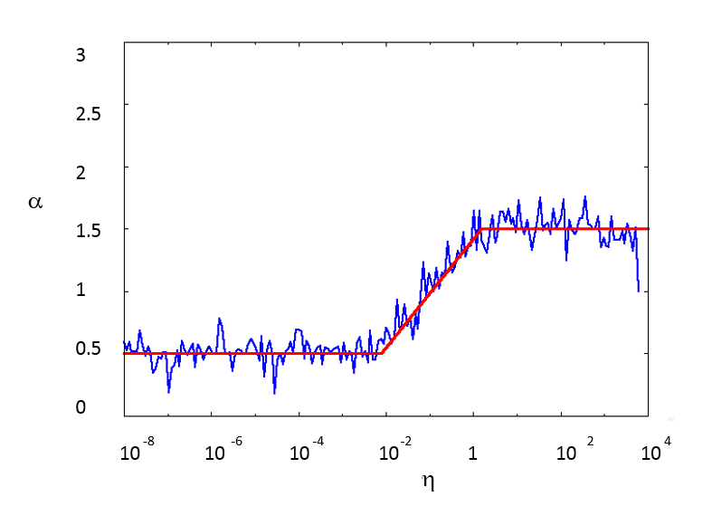
Figure 1: Plot of the exponent $\alpha$ for the fit $\sigma(t)=C\,\epsilon\,n^{\alpha}$ to the forward error of the anharmonic oscillator with a stochastic perturbation of amplitude $\epsilon$ as a function of the nonlinearity strength $\eta$. The noise is additive in Cartesian coordinates, according to equation (70). The red line is drawn just to guide the eye. When $\eta\ll 1$ the system is almost isochronous and $\alpha=1/2$, when $\eta\gg 1$ the system is strongly anisochronous and $\alpha=3/2$, but in the intermediate region the exponent varies continuously between these two values.

In these new coordinates the noise become multiplicative. A much simpler model to solve analytically is the one in which the noise is additive

$$H=H_{0}(J)\,-\Theta\,\epsilon\,e_{J}\,\xi_{J}(t)+J\,\epsilon\,e_{\Theta}\,\xi_{\Theta}(t)\qquad\qquad H_{0}(J)=\omega J+\eta\,{3\over 8}\,{J^{2}\over\omega^{2}}$$

where ${\mathbf{e}}=(e_{\Theta},e_{J})$ is a unit vector and $\xi_{\Theta}$, $\xi_{J}(t)$ are independent white noises.

In this case the equations of motion can be solved explicitly by retaining only the first order in $\epsilon$ and for initial conditions $J(0)=J_{0},\,\Theta(0)=\Theta_{0}$ read

$$\Theta=\Theta_{0}+\Omega(J_{0})t+\epsilon\Omega^{\prime}(J_{0})\,e_{J}\,w_{J}^{(1)}(t)\,+\epsilon\,e_{\theta}\,w_{\theta}(t)\qquad\qquad J(t)=J_{0}+\epsilon\,e_{J}\,w_{J}(t)$$

where $\Omega=dH_{0}/dJ$ and $\Omega^{\prime}=d\Omega/dJ$ . As long as the distance on the cylinder agrees with the Euclidean distance we can write for the forward error

$$\sigma(t)=\epsilon\left[{{t+e_{J}^{2}\,{\Omega^{\prime}}^{2}(J_{0})\,t^{3}/3}}\right]^{1/2}$$

The figure shows the result of a fit to the exponent $\alpha$ for power law growth of the forward error $\sigma(t)=C\epsilon\,t^{\alpha}$ as a function of the anisochronicity strength $\eta$. The function $\alpha(\eta)$ varies between $1/2$ and $3/2$ with a rather sharp transition in agreement with theoretical estimate (74).

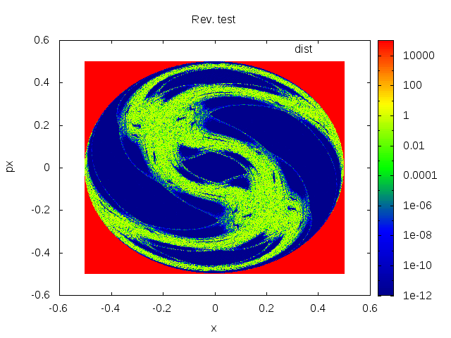
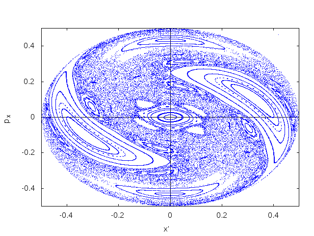
Figure 2: Hénon-Heiles non integrable Hamiltonian $H_{-}$ given by equation (75). Left side: colour plot of the reversibility error due to round off for $H_{-}=1/8$ and initial conditions on a grid of points in the $(x,p_{x})$, with $y=0,p_{y}>0$ and $t=100$ dynamic periods $T=2\pi$. Right figure: phase space plot for the projection into the $(x,p_{x})$ phase plane of the orbits in the Poincaré section $y=0,p_{y}>0$

7.2 The Hénon Heiles Hamiltonian

This model describes the motion of an elliptical galaxy and the Hamiltonian reads

$$H_{\pm}={1\over 2}(p_{x}^{2}+p_{y}^{2})+{1\over 2}(x^{2}+y^{2})+x^{2}y\pm{1\over 3}y^{3}$$

The Hamiltonian $H_{-}$ is not integrable, whereas the model $H_{+}$ is integrable. For the first one we have considered the reversibility error due to the round off. In Figure 2 we compare the colour plot for the reversibility error with the phase portrait. Both refer to the Poincaré section $y=0,\dot{y}>0$

7.3 The N vortex model

For inviscid plane fluid the dynamics of point vortices provides a complete description of the dynamic evolution. The Hamiltonian for $N$ point vortices located at $z_{k}=x_{k}+iy_{k}$ with a strength $\Gamma_{k}$ is

$$H({\mathbf{x}})=-{1\over 4\pi}\,\sum_{j\not=k}\,\Gamma_{j}\Gamma_{k}\log|z_{j}-z_{k}|$$

The coordinates $x_{k}$ and $y_{k}$ are canonically conjugated.

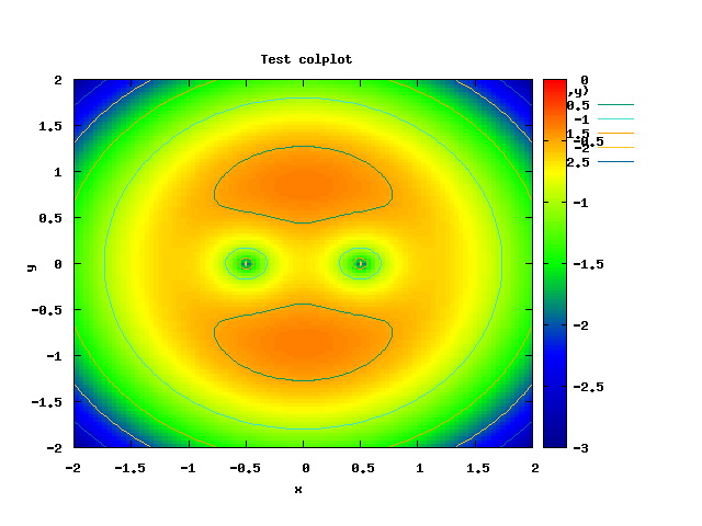
Figure 3: Level lines and isocolor for the three vortices Hamiltonian in the symmetric case $\lambda=1/2$

There are two independent first integrals in involution. As a consequence the system of 3 vortices is integrable, while a system of 4 is not . If the vorticity of one of them is very low, a reduced Hamiltonian can be written which looks similar to the restricted planar three body problem. Introducing a canonical change of coordinates the Hamiltonian reads

$$H=-{1\over 2}(x^{2}+p^{2})+(1-\lambda)\log[(x+\lambda)^{2}+p^{2}]^{1/2}+\lambda\log[(x+\lambda-1)^{2}+p^{2}]^{1/2}$$

We remark that the splitting cannot be used to construct an explicit symplectic integrator. Only symplectic implicit schemes are available. However one can use a 4-th order Runge-Kutta integrator choosing $n_{s}=10^{4}$ such that the Hamiltonian is conserved within an error very small with respect to the stochastic perturbation. In Figure 3 we show level curves of the Hamiltonian (77). The behaviour of the forward and reversibility error follows the power law with exponent $3/2$ in agreement with the theory.

8 The observational noise

To complete the present analysis on the effect of noise on a dynamical system we consider now the effect of observations. We suppose they are made regularly with a time interval $T$. We assume our system to be regular and to be given by the translation on the torus ${\mathbb{T}}$ and that each observation, having a small duration $\tau\ll T$, behaves as a white noise of amplitude $\epsilon$. The correlation and the fidelity for an observable $f_{\mathbb{T}}(x)$ during the first measurement $T<t<T+\tau$ decay. After this time interval the correlation oscillates, whereas the fidelity remains constant, namely for $t>T+\tau$ is

$$C_{\epsilon}(t)=\sum_{k\not=0}\,\,|f_{k}|^{2}e^{2\pi\,i\,\omega\,t}\,e^{-2\pi^{2}\epsilon^{2}\tau}\qquad\qquad F_{\epsilon}(t)=\sum_{k\not=0}\,\,|f_{k}|^{2}e^{-2\pi^{2}\epsilon^{2}\tau}$$

If we repeat measurements of the same duration $\tau$ and same time separation $T$, after $n$ of them, namely for $t\geq n(T+\tau)$, the decrease factor $e^{-2\pi^{2}\,\epsilon^{2}\,n\tau}$ becomes significant if $n\,\epsilon^{2}\tau>1$. The threshold $t_{*}$ to observe the exponential decrease is

$$t_{*}\sim{T\over\epsilon^{2}\,\tau}$$

8.1 Map formulation

If the disturbance introduced by the measurement is proportional to the signal itself, then we must treat it as a multiplicative noise. In the continuous time case analytical estimates are difficult to obtain also for translations on the torus. To overcome the difficulty we consider the case of a discrete time system. When the noise is additive the results are similar to the continuous time case. We consider a map $M$ which gives the evolution on the same time interval $T$ which separates two subsequent observations. Letting $x_{n+1}=M(x_{n})$ we have

$$x_{n}=x_{n-1}+\omega T+\epsilon\,\tau^{1/2}\,\xi_{n}\,\,\mbox{mod}\,1$$

where $\xi_{n}$ are random variables uniformly distributed in $[-1,1]$. The correlation after $n=1$ iteration (observation) is

$$\eqalign{C_{\epsilon}(1)&=\int_{0}^{1}dx_{0}\,f_{\mathbb{T}}(x_{0})\,\langle f_{{\mathbb{T}}}(x_{0}+\omega T+\epsilon\,\tau^{1/2}\xi)\rangle=\cr&=\sum_{k,k^{\prime}\not=(0,0)}\,f_{k}f_{-k^{\prime}}\,e^{2\pi\,i\,k\,\omega T}\,{1\over 2}\,\int_{-1}^{1}\,d\xi\,e^{2\pi\,i\,k\epsilon\,\tau^{1/2}\,\xi}\times\int_{0}^{1}\,dx_{0}\,e^{2\pi(k^{\prime}-k)x_{0}}=\cr&=\sum_{k\not=}\,|f_{k}|^{2}\,\,e^{2\pi\,i\,k\,\omega T}\,S(\epsilon\,\tau^{1/2}\,k)\qquad\qquad S(x)={\sin(2\pi x)\over 2\pi x}\cr}$$

After $n$ iterations (observations) the correlation becomes

$$C_{\epsilon}(n)=\sum_{k\not=}\,|f_{k}|^{2}\,\,e^{2\pi\,i\,kn\omega T}\,S^{n}(\epsilon\,\tau^{1/2}k)$$

The same result holds for the fidelity where the phase factor is absent. We recall that $|S(x)|\leq e^{-x^{2}\log(2\pi)}$ for $|x|\leq 1$ and $|S(x)|\leq(2\pi|x|)^{-1}$ for $|x|>1$, see reference [13], and follow the same procedure outlined there. Assuming $\epsilon\,\tau^{1/2}\ll 1$ and that the Fourier coefficients are bounded by $|f_{k}|\leq A/|k|$, we have

$$|C(n)|\leq 2A^{2}\,e^{-n\,\tau\,\epsilon^{2}\,\log(2\pi)}$$

8.2 Multiplicative noise

If the random perturbation introduced by an observation is proportional to the signal effect and we make a single observation after $N$ iterations the map (82) is replaced by

$$x_{n}=(x_{n-1}+\omega\,T)(1+\epsilon\,\tau^{1/2}\xi_{n})\,\,\mbox{mod}\,1$$

After the first iteration the correlation reads

$$\eqalign{C_{\epsilon}(1)&=\sum_{k,k^{\prime}\not=(0,0)}\,f_{k}f_{-k^{\prime}}\,e^{2\pi\,i\,k\omega T}\,{1\over 2}\,\int_{-1}^{1}\,d\xi\,e^{2\pi\,i\,k\,\omega T\,\epsilon\tau^{1/2}\xi}\int_{0}^{1}\,dx_{0}\,e^{2\pi\,i\,(k(1+\epsilon\tau^{1/2}\xi)-k^{\prime})x_{0}}=\cr&=\sum_{k,k^{\prime}\not=(0,0)}\,f_{k}f_{-k^{\prime}}(-1)^{k-k^{\prime}}\,e^{2\pi\,i\,k\omega T}\,{1\over 2}\,\int_{-1}^{1}\,d\xi\,S\left({{k-k^{\prime}+k\epsilon\tau^{1/2}\xi\over 2}}\right)\cdot\cr&\cdot\exp\left({{2\pi\,i\,k\epsilon\tau^{1/2}\xi\left({{\omega T+{1\over 2}}}\right)}}\right)\cr}$$

If $f_{\mathbb{T}}(x)$ is a trigonometric polynomial, namely $f_{k}=0$ for $|k|\geq K$ and $\epsilon\tau^{1/2}K\ll 1$ then $S((k-k^{\prime}-k\epsilon\tau^{1/2}\xi)/2)\sim\delta_{k,k^{\prime}}$ so that

$$C_{\epsilon}(1)=\sum_{k\not=0}\,|f_{k}|^{2}\,e^{2\pi\,i\,kn\omega T}\,S\left({{k\epsilon\tau^{1/2}\left({{\omega T+{1\over 2}}}\right)}}\right)$$

Supposing that $\epsilon\tau^{1/2}\,\omega T\gg 1$ a single observation produces a significant decrease in the correlation roughly proportional to $(\tau^{1/2}\,\epsilon\,\omega T)^{-1}$. On the contrary if $\epsilon\tau^{1/2}\,\omega T\ll 1$ the decrease is negligible and we need to make several observations. After $n$ observations we have

$$C_{\epsilon}(n)=\sum_{k\not=0}\,|f_{k}|^{2}(-1)^{k-k^{\prime}}\,e^{2\pi\,i\,kn\omega T}\,S^{n}\left({{k\,\tau^{1/2}\epsilon\left({{\omega T+{1\over 2}}}\right)}}\right)$$

Supposing that $\tau^{1/2}\epsilon\ll 1$ and $\omega T\gg 1$ we have the following estimates

$$C_{\epsilon}(n)\leq 3A^{2}\cases{\exp\left({{-\log(2\pi)\,n\tau\epsilon^{2}(\omega T)^{2}}}\right)&if $\tau^{1/2}\epsilon\,\omega T\ll 1$\cr&\cr(2\pi\,\tau^{1/2}\epsilon\,\omega T)^{-n}&if $\tau^{1/2}\epsilon\,\omega T\gg 1$\cr}$$

To conclude, if the stochastic perturbation, introduced by an observation, is multiplicative rather than additive, a phase factor $\omega T$ is introduced in the correlation decay. Since the perturbation amplitude and duration are assumed to be small ($\tau^{1/2}\epsilon\ll 1$), if the phase factor is large ($\omega T\gg 1$), the decay is much faster. If $\tau^{1/2}\epsilon\omega T\sim 1$, a few observations determine a significant decay of correlations in the multiplicative case.

9 Conclusions

We have examined the asymptotic behaviour of the forward and reversibility errors (FE, RE) introduced by stochastic perturbations in a dynamical system defined on a compact phase space and we have compared these errors with the decay rates of correlation and fidelity. We have first considered the translations on the torus ${\mathbb{T}}$ and the cylinder, showing that both errors follow the same power law with an exponent equal to $1/2$ and $3/2$ respectively. For expanding flows on ${\mathbb{T}}$ the FE grows exponentially, but the equivalence of FE and RE occurs only if we have a linear flow on the torus $T^{2}$ which preserves the area. This is a special case of linear Hamiltonian flows for which the asymptotic equivalence of FE and RE is proved. We have analysed the relation between the memory loss and the error growth. For linear Hamiltonian systems we have shown that the correlation and fidelity decay as $e^{-2\pi^{2}\sigma^{2}(t)}$ where $\sigma(t)$ is the FE and that a similar relation holds between the fidelity and the RE. The RE method can be used to investigate the transition regions from regular to chaotic motions and the effect of round off errors in numerical simulations. The proposed framework is general and an extension to classical fields, by using the theory of linear stochastic partial differential equations to define the FE and RE, could be considered. Finally we have examined the effect of the observational noise showing that for an integrable system only a sequence of observations can lead to the decay of the correlation and that the multiplicative noise can increase the decay rate if the phase advance between two observations is large.

Appendix A Correlation on the torus and Perron Frobenius operator

Given a map $M(x)$ continuous on the torus there is a unique definition of correlation. Indeed the evolution of a given initial distribution $f_{\mathbb{T}}(x)$ is governed by the Perron Frobenius equation

$$f_{\mathbb{T}}(x,n)=({\mathsf{P}}^{n}f_{\mathbb{T}})(x)=\int_{0}^{1}\,\delta(x-M^{n}(x_{0}))f_{{\mathbb{T}}}(x_{0})dx_{0}=\sum_{j=1}^{q^{n}}{f_{{\mathbb{T}}}(x_{j})\over(M^{n})^{\prime}(x_{j})}$$

where ${\mathsf{P}}$ is the Perron-Frobenius operator. Supposing $M(x_{0})$ has $q$ preimages, with $x_{j}=(M^{-n})_{j}(x)$ for $1\leq j\leq q^{n}$ we have indicated all the preimages of $M^{n}(x_{0})$. For any $A\subset{\mathbb{T}}^{1}$ the invariance of the probability measure $\mu$ is expressed by $\mu(M^{-1}(A))=\mu(A)$. For example the Bernoulli map $M(x)=qx\,\,\mbox{mod}\,1$ where $q\in{\mathbb{N}}$ has $q$ inverses and $M^{-1}\equiv\cup_{k}M^{-1}_{k}(A)$ where $\mu(M^{-1}_{k}(A))=q^{-1}\mu(A)$. Since the density of the absolutely continuous invariant measure is 1, we define the correlation according to

$$\eqalign{C(n)&=\int_{0}^{1}\,f_{\mathbb{T}}(x_{0})f_{\mathbb{T}}(M^{n}(x_{0}))\,dx_{0}-f_{0}^{2}=\cr&=\int_{0}^{1}\,dx_{0}\,f_{\mathbb{T}}(x_{0})\int_{0}^{1}\delta(x-M^{n}(x_{0}))\,f_{\mathbb{T}}(x)\,dx-f_{0}^{2}=\cr&=\int_{0}^{1}\,f_{\mathbb{T}}(x)f_{\mathbb{T}}(x,n)\,dx-f_{0}^{2}\cr}$$

where the result has been obtained by interchanging the integration order.

As a specific example we consider the linear map $M(x)=qx\,\,\mbox{mod}\,1$ continuous on ${\mathbb{T}}$ for integer $q$. In this case the preimages $x_{j}$ of $M^{n}$ are

$$x_{j}=(M^{-n})_{j}(x)={x\over q^{n}}+{j_{n}\over q}+{j_{n-1}\over q^{2}}+\ldots+{j_{2}\over q^{n-1}}+{j_{1}\over q^{n}}={x+j\over q^{n}}$$

where $j_{i}=0,1,\ldots,q-1$ and $j=j_{1}+qj_{2}+\ldots+q^{n-2}\,j_{n-1}+q^{n-1}j_{n}$ has a range from $0$ to $q^{n}-1$. As a consequence, from the Perron-Frobenius equation we have

$$f_{\mathbb{T}}(x,n)=\sum_{j=0}^{q^{n}-1}\,q^{-n}\,f_{\mathbb{T}}(q^{-n}(x+j)$$

and the following equality can be proved

$$\eqalign{&\int_{0}^{1}\,f_{\mathbb{T}}(x,n)\,f_{\mathbb{T}}(x)\,dx=\sum_{0}^{q^{n}-1}\,\int_{0}^{1}\,{1\over q^{n}}\,f_{\mathbb{T}}\left({{x+j\over q^{n}}}\right)\,f_{\mathbb{T}}(x)=\cr&=\sum_{j=0}^{q^{n}-1}\int_{j/q^{n}}^{(j+1)/q^{n}}\,dx_{0}\,f_{\mathbb{T}}(x_{0})\,f_{\mathbb{T}}\left({{q^{n}\,x_{0}-j}}\right)\,=\int_{0}^{1}\,dx_{0}f_{\mathbb{T}}(x_{0})\,f_{\mathbb{T}}(q^{n}x_{0})\cr}$$

where we have made the coordinates change $x+j=q^{n}x_{0}$. Letting $f_{k}$ be the Fourier coefficients of $f_{\mathbb{T}}(x)$ the order $k$ Fourier coefficients of $f_{\mathbb{T}}(x,n)$ are $f_{k}(n)=f_{q^{n}k}$. The equality (A4) is a consequence of continuity of the map $M$ on ${\mathbb{T}}$. For a linear flow $S_{t}(x_{0})=e^{\beta t}\,x_{0}$ we have seen that a similar equality, given by equation (22), holds only for the sequence of values of $t_{m}$ such that $e^{\beta t_{m}}=m$ is an integer, since the map $S_{t_{m}}(x_{0})=m\,x_{0}\,\hbox{mod}\,1$ is continuous on ${\mathbb{T}}$.