Homoclinic snaking in plane Couette flow: bending, skewing, and finite-size effects

Abstract

Invariant solutions of shear flows have recently been extended from spatially periodic solutions in minimal flow units to spatially localized solutions on extended domains. One set of spanwise-localized solutions of plane Couette flow exhibits homoclinic snaking, a process by which steady-state solutions grow additional structure smoothly at their fronts when continued parametrically. Homoclinic snaking is well understood mathematically in the context of the one-dimensional Swift-Hohenberg equation. Consequently, the snaking solutions of plane Couette flow form a promising connection largely phenomenological study of laminar-turbulent patterns in viscous shear flows and the mathematically well-developed field of pattern-formation theory. In this paper we present a numerical study of the snaking solutions, generalizing beyond the fixed streamwise wavelength of previous studies. We find a number of new solution features, including bending, skewing, and finite-size effects. We show that the finite-size effects result from the shift-reflect symmetry of the traveling wave and establish the parameter regions over which snaking occurs. A new winding solution of plane Couette flow is derived from a strongly skewed localized equilibrium.

1 Introduction

Invariant solutions of the Navier-Stokes equations are known to play an important role in the dynamics of turbulence at low Reynolds numbers (Kawahara et al., 2012). These solutions, in the form of equilibria, traveling waves, and periodic orbits, have been computed precisely for canonical shear flows such as pipe flow (Faisst & Eckhardt, 2003; Wedin & Kerswell, 2004; Duguet et al., 2008), plane Couette flow (Nagata, 1990; Kawahara & Kida, 2001; Viswanath, 2007; Gibson et al., 2009) and plane Poiseuille flow (Waleffe, 2001; Gibson & Brand, 2014). The development of the invariant-solutions approach to turbulence has largely occurred in the simplified context of small, periodic domains, or ‘minimal flow units’ (Jiménez & Moin, 1991). More recently, invariant solutions with localized support have been computed for flows on spatially extended domains. These include spanwise-localized equilibria and traveling waves (Schneider et al., 2010b, a; Deguchi et al., 2013; Gibson & Brand, 2014) in plane Couette flow, and spanwise-localized traveling waves (Gibson & Brand, 2014) and a periodic orbit (Zammert & Eckhardt, 2014a) of plane Poiseuille flow. Avila et al. (2013) computed a streamwise-localized periodic orbit of pipe flow, Mellibovsky & Meseguer (2015) a streamwise-localized periodic orbit of plane Poiseuille flow, Brand & Gibson (2014) a doubly-localized equilibrium solution of plane Couette flow, and Zammert & Eckhardt (2014b) a doubly-localized periodic orbit of plane Poiseuille flow. The existence and structure of these spatially localized solutions suggests that they are relevant to large-scale patterns of laminar-turbulent intermittency, such as turbulent stripes, spots, and puffs. For example, the periodic orbit of Avila et al. (2013) shares the spatial structure and complexity of turbulent puffs in pipe flow, and its bifurcation sequence provides a compelling explanation of the development of transient turbulence in pipes. The doubly-localized equilibrium of Brand & Gibson (2014) has the characteristic shape and structure of turbulent spots in low-Reynolds plane Couette flow, and for a range of Reynolds numbers sits on the boundary between laminar flow and turbulence. Analysis of these localized solutions has so far focused on their bifurcations from spatially periodic solutions (Chantry et al., 2014; Mellibovsky & Meseguer, 2015) and linear analysis of their decaying tails (Brand & Gibson, 2014; Gibson & Brand, 2014).

The spanwise-localized invariant solutions of plane Couette flow of Schneider et al. (2010b), are notable for being the first localized solutions discovered, for their relation to the widely-studied equilibrium solution of Nagata (1990); Clever & Busse (1997); Waleffe (1998) (hereafter NBCW), and for exhibiting the particularly interesting feature of homoclinic snaking. Homoclinic snaking is a process by which the localized solutions grow additional structure at their fronts in a sequence of saddle-node bifurcations when continued parametrically (Knobloch (2015); Schneider et al. (2010a); see also § 3.1). Homoclinic snaking occurs a number of pattern-forming systems with localized solutions, including binary fluid convection (Batiste & Knobloch, 2005) and magneto-convection (Batiste et al., 2006), and it is well-understood mathematically for the one-dimensional Swift-Hohenberg equation (Burke & Knobloch, 2007; Beck et al., 2009). Knobloch (2015) provides a comprehensive review of localization and homoclinic snaking in dissipative systems. Though no explicit connection between the Swift-Hohenberg and the Navier-Stokes equations is known, the striking similarity of the localized plane Couette solutions and the localized solutions of Swift-Hohenberg with cubic-quintic nonlinearity suggests there might be a mathematical connection between the two systems. These similarities include the structure of localization, the snaking behaviour, the even/odd symmetry of the snaking solutions, and the existence of asymmetric rung solutions (Schneider et al., 2010a). One might envision, for example, that a reduced-order model of the localized solutions (Hall & Sherwin, 2010; Hall, 2012; Beaume et al., 2015) might relate the spanwise variation of their mean streamwise flow to the cubic-quintic Swift-Hohenberg equation. Such a relation would link the mathematically well-developed field of pattern-formation theory to the localized solutions of shear flows cited above, or to recent numerical studies of laminar-turbulent pattern formation in extended shear flows (Barkley & Tuckerman, 2005; Duguet et al., 2010; Tuckerman et al., 2014).

In support of developing such connections between pattern-formation theory and shear flows, we present in this paper a more detailed analysis of the snaking solutions of Schneider et al. (2010b, a). In particular, we examine the effects of varying the streamwise wavelength $L_{x}$ of the solutions compared to the fixed $L_{x}=4\pi$ of Schneider et al. (2010a). We find that homoclinic snaking is robust in $L_{x}$ and that the snaking region moves upwards in Reynolds number with decreasing $L_{x}$. The ranges of streamwise wavelength and Reynolds number in which snaking solutions exist is found to be $1.7\pi\leq L_{x}\leq 4.2\pi$ and $165\leq\mathrm{Re}\leq 2700$. Additionally, we find several interesting solution properties that are suppressed at the parameters studied in Schneider et al. (2010a). As $L_{x}$ as decreases below $4\pi$ and $\mathrm{Re}$ increases above $165$, the localized solutions deform appreciably compared to their strictly periodic counterparts, the localized equilibria exhibiting a linear skewing and the traveling waves a quadratic bending. We show that skewing and bending are related to the respective symmetries of the equilibrium and traveling wave solutions, and that bending induces finite-size effects in the traveling waves that scale as the inverse of their spanwise width. In contrast, skewing induces no such finite-size effects on the equilibrium solution. We show that the skewed solutions lead to a new periodically winding form of the NBCW equilibrium solution of plane Couette flow.

The structure of this paper is as follows. Sec. 2 outlines the problem formulation and numerical methods. Sec. 3 describes the features of the localized solutions at fixed streamwise wavelength $L_{x}$, including homoclinic snaking, bending, skewing, and finite-size effects. Sec. 4 discusses the effects of varying streamwise wavelength, including the regions of wavelength and Reynolds number over which snaking occurs, the breakdown of snaking outside these regions, and the stability of the solutions. Sec. 5 discusses the periodic pattern in the interior of the localized solutions and its relation to the NBCW solution. The new winding solution is also presented in § 5.

2 Problem formulation, methodology, and conventions

Plane Couette flow consists of an incompressible Newtonian fluid between two infinite parallel plates moving at constant relative velocity. The Reynolds number is given by $\mathrm{Re}=Uh/\nu$ where $U$ is half the relative wall speed, $h$ is half the distance between the walls, and $\nu$ is the kinematic viscosity. The ${\bf x}=(x,y,z)$ coordinates are aligned with the streamwise, wall-normal, and spanwise directions, where streamwise is defined as the direction of relative wall motion. After nondimensionalization the walls at $y=\pm 1$ move at speeds $\pm 1$ in the $x$ direction, and the laminar velocity field is given by $y{\bf e}_{x}$. We decompose the total fluid velocity into a sum of the laminar flow and the deviation from laminar: ${\bf u}_{\text{tot}}=y{\bf e}_{x}+{\bf u}$. Hereafter we refer to the deviation field ${\bf u}({\bf x},t)=[u,v,w](x,y,z,t)$ as “velocity.” In these terms the laminar solution is specified by ${\bf u}=0$, $p=0$ and the Navier-Stokes equations take the form

$$\frac{\partial{\bf u}}{\partial t}+y\frac{\partial{\bf u}}{\partial x}+v{\bf e}_{x}+{\bf u}\cdot{\bf\nabla}{\bf u} =-{\bf\nabla}p+\frac{1}{\mathrm{Re}}\nabla^{2}{\bf u},\quad{\bf\nabla}\cdot{\bf u}=0.$$ (1)

The computational domain $\Omega=[-L_{x}/2,\>L_{x}/2]\times[-1,1]\times[-L_{z}/2,\>L_{z}/2]$ has periodic boundary conditions in $x$ and $z$ and no-slip conditions at the walls. For spanwise-localized solutions, $L_{z}$ is typically large, so that $\Omega$ approximates a spanwise-infinite domain. We use $\hat{L}_{z}$ to denote the spanwise wavelength of nearly periodic, small-wavelength patterns within the spanwise-localized solutions; typically $\hat{L}_{z}\ll L_{z}$. In the present work we impose zero mean pressure gradient in all computations, leaving the mean (bulk) flow to vary dynamically. As described in Gibson et al. (2008, 2009), direct numerical simulations are performed with Fourier-Chebyshev spatial discretization and semi-implicit time-stepping, traveling-wave and equilibrium solutions of (1) are computed with a Newton-Krylov-hookstep algorithm, and all software and solution data is available for download at www.channelflow.org.

The equilibrium and traveling-wave solutions discussed here are all steady states (in a fixed or traveling frame of reference, respectively), so the energy dissipation rate balances the power input from wall shear instantaneously:

$$D=I=\frac{1}{2L_{x}}\int_{-L_{x}/2}^{L_{x}/2}\int_{-L_{z}/2}^{L_{z}/2}\left.\frac{\partial u}{\partial y}\right|_{y=-1}+\left.\frac{\partial u}{\partial y}\right|_{y=1}dx\,dz.$$ (2)

Note that $D$ is defined in terms of the deviation velocity ${\bf u}$ and not the total velocity ${\bf u}_{\text{tot}}$, so that $D$ measures the excess energy dissipation of spanwise-localized solutions over the laminar flow, which has $D=0$. Since the internal structure of a spanwise-localized solutions stays roughly constant as non-laminar structure grows at its fronts, $D$ serves as a good measure of the width of a solution. The lack of $L_{z}$ normalization makes the $D$ of a spanwise-localized solution insensitive to the choice of spanwise length for the computational domain in which it is embedded.

For discussing the symmetries of the flow we follow the conventions of Gibson & Brand (2014), here adding the action of symmetries on the pressure field. Let

$$\sigma_{x} :[u,v,w,p](x,y,z)\rightarrow[-u,v,w,p](-x,y,z),$$

$$\sigma_{y} :[u,v,w,p](x,y,z)\rightarrow[u,-v,w,p](x,-y,z),$$

$$\sigma_{z} :[u,v,w,p](x,y,z)\rightarrow[u,v,-w,p](x,y,-z),$$

$$\tau(\Delta x,\Delta z) :[u,v,w,p](x,y,z)\rightarrow[u,v,w,p](x+\Delta x,\,y,\,z+\Delta z),$$ (3)

and let concatenation of subscripts indicate products, e.g. $\sigma_{xy}=\sigma_{x}\sigma_{y}$. For $(\ell_{x},\ell_{z})$-periodic fields we define two half-wavelength translation operators $\tau_{x}=\tau(\ell_{x}/2,0)$ and $\tau_{z}=\tau(0,\ell_{z}/2)$. The standard group-theoretic angle-bracket notation indicates the group formed by a set of generators; for example $\langle\sigma_{xy},\tau_{x}\sigma_{z}\rangle=\{e,\,\sigma_{xy},\,\tau_{x}\sigma_{z},\,\tau_{x}\sigma_{xyz}\}$, where $e$ is the identity (Dummit & Foote, 2004).

3 Solution properties at fixed streamwise wavelength

3.1 Snaking

(a) (b)

Figure 1: Homoclinic snaking of localized solutions at $L_{x}=3\pi$ (details). (a) Snaking curves at low $D$ (small spanwise width) for localized equilibrium (EQ), traveling-wave (TW), and rung (RN) solutions. Labels indicate the solutions shown as velocity fields in fig. 2. (b) Snaking curves at high $D$ (large spanwise width). Filled circles indicate the points of zero skewing (for equilibria) and zero bending (for traveling waves) along the snaking curves; signed open circles mark the positions and signs of the maxima in magnitude of skewing and bending (see § 3.3). Pressure fields for the labeled points are shown in fig. 3. Both subplots are details of the $L_{x}=3\pi$ snaking curve shown in fig. 4(d).

The primary notable feature of the localized solutions is their homoclinic snaking. Under continuation in Reynolds number at fixed streamwise wavenumber, the localized equilibrium and traveling-wave solutions follow curves that snake upwards in the $\mathrm{Re},D$ plane, as shown in detail in fig. 1 and over a larger range of $D$ in fig. 4(d). Velocity fields corresponding to the labeled points in fig. 1(a) are shown in fig. 2. Figs. 2(a,b,c) show that the traveling-wave solution grows additional structure at the solution fronts as it moves upwards in $D$ along the snaking curve, while the interior structure remains nearly constant. The structure of the fronts is the same at alternating saddle-node points (a,c), while the saddle-node point (b) between them has front structure of opposite streamwise sign. Note that due to the $\sigma_{xy}$ symmetry of plane Couette flow, every traveling-wave solution ${\bf u}$ with wave speed $c_{x}$ has a symmetric partner $\sigma_{xy}{\bf u}$ with wave speed $-c_{x}$. The $\sigma_{xy}{\bf u}$ symmetric partner of fig. 2(b) has fronts with the same structure and streamwise sign as fig. 2(a,c).

Fig. 1(a) also shows “rung” solutions that bifurcate from the equilibrium solution in a pitchfork bifurcation near the saddle-node bifurcation points of the equilibrium and connect to the traveling wave near their saddle-node points (or vice versa). The existence of the rung solutions can be understood from a physical viewpoint as a combination of two solutions near the saddle-node bifurcation point, with different widths $D$ but the same Reynolds number. For example, the equilibria marked 2d and 2f in fig. 1(a) and depicted as streamwise velocity fields in fig. 2(d,f) are indistinguishable within the interior $-5<z<5$. But their differing values of $D$ indicate different spanwise lengths. The contour lines of the fronts of 2(f) extend towards $|z|\approx 10$, whereas those of 2(d) reach just $|z|\approx 8$. The rung solution shown as fig. 2(e) and marked 2e in fig. 1(a) can then be understood as splicing together the left half of fig. 2(d) and the right half of fig. 2(f). This splicing can be done at arbitrary $\mathrm{Re}$ in the interior of the saddle-node bifurcation, i.e. along the black lines of the rung branches shown fig. 1(a). The splicing construction is necessarily imperfect, since the rung solutions have no symmetries and hence travel in both $x$ and $z$, compared to the equilibrium, which is fixed. However it is close enough that such spliced velocity fields converge quickly to the rung solutions under Newton-Krylov-hookstep search. The rung solutions in this paper were computed by splicing and refinement, followed by continuation in Reynolds number.

(a) (d)
        
(b) (e)
        
(c) (f)

Figure 2: (color online) Velocity fields of localized solutions illustrated by contours of streamwise velocity in the $y=0$ midplane, $u(x,0,z)$ and arrow plots of the streamwise-averaged cross-stream velocity, $[\bar{v},\bar{w}](y,z)$. Eight contour levels are evenly spaced between $\pm 0.9$, with negative $u$ in dashed blue lines and positive in solid red. Contour lines for $\bar{u}=0$ are superimposed on the arrow plots. (a,b,c) show the traveling-wave (TW) solution at the three successive lower saddle-node bifurcation points marked on the snaking curve in fig. 1(a). (e,f) show the equilibrium (EQ) solution at $\mathrm{Re}=260$ above and below an upper saddle-node bifurcation, and (d) shows the rung solution at $\mathrm{Re}=260$, at points labeled in fig. 1(a). The solution is shown for $L_{x}=3\pi$ and on a subset of the $L_{z}=16\pi$ computational domain.

3.2 Symmetries of localized solutions

The differences between traveling waves, equilibria, and rungs are intimately related to the different symmetries of those solutions, which can be understood in terms of symmetry-breaking bifurcations of the more symmetric, spatially periodic NBCW solution. This is discussed in detail in Gibson & Brand (2014); here we present a brief summary. With proper placement of the $z$ origin, the traveling waves have a $\tau_{x}\sigma_{z}$ “shift-reflect” symmetry. That is, a traveling-wave solution satisfies ${\bf u}=\tau_{x}\sigma_{z}{\bf u}$ or

$$[u,v,w,p](x,y,z)=[u,v,-w,p](x+\ell_{x}/2,y,-z).$$ (4)

Solutions with this symmetry can travel in $x$ but not $z$, since the inversion in $z$ about the origin locks the $z$ phase of the solution, but no such restriction exists for $x$. For similar reasons, the traveling waves can have nonzero mean streamwise velocity, but their mean spanwise velocity must be zero. The $\tau_{x}\sigma_{z}$ symmetry of the localized traveling waves arises from a subharmonic-in-$z$ bifurcation of the $(\ell_{x},\ell_{z})$-periodic NBCW solution, which in the spatial phase of Waleffe (2003), has symmetries $\langle\tau_{x}\sigma_{z},\tau_{xz}\sigma_{xy}\rangle$. The subharmonic-in-$z$ bifurcation necessarily breaks the $\tau_{xz}\sigma_{xy}$ symmetry, since this symmetry implies $\ell_{z}$ periodicity, as follows. If $\tau_{xz}\sigma_{xy}{\bf u}={\bf u}$, then $(\tau_{xz}\sigma_{xy})^{2}{\bf u}={\bf u}$. But a brief calculation shows that $(\tau_{xz}\sigma_{xy})^{2}=\tau(0,\ell_{z})$. Thus the bifurcated solution loses the $\tau_{xz}\sigma_{xy}$ symmetry of NBCW and retains only $\tau_{x}\sigma_{z}$.

The localized equilibrium solution has $\sigma_{xyz}$ inversion symmetry, satisfying

$$[u,v,w,p](x,y,z)=[-u,-v,-w,p](-x,-y,-z).$$ (5)

As a result of the inversion of all velocity components about the origin, the spanwise-localized solutions with this symmetry is prevented from traveling in $x$ or $z$, and the spatial average of all velocity components is zero. The $\sigma_{xyz}$ symmetry of the localized equilibrium arises from a similar bifurcation of a phase-shifted NBCW solution. Shifting the NBCW solution by a quarter-wavelength in $z$, ${\bf u}\rightarrow\tau_{z}^{1/2}{\bf u}$, changes each of its symmetries $s$ to the conjugate symmetry $\tau_{z}^{-1/2}s\tau_{z}^{1/2}$ (Gibson et al., 2009). A brief calculation shows that the conjugated symmetry group of the phase-shifted NBCW solution is $\langle\tau_{xz}\sigma_{xy},\sigma_{xyz}\rangle$. The $\tau_{xz}\sigma_{xy}$ symmetry implies $\ell_{z}$-periodicity, as before, so the subharmonic-in-$z$ bifurcation breaks the $\tau_{xz}\sigma_{xy}$ symmetry but retains $\sigma_{xyz}$.

The symmetries of the traveling-wave and equilibrium solutions and the lack of symmetry in rung solutions are evident in the velocity-field plots shown in fig. 2. The $z$-mirror, $x$-shift $\tau_{x}\sigma_{z}$ traveling-wave symmetry (4) is particularly apparent in the fronts of the midplane $u$ contour plots of fig. 2(a,b,c), and an even $z$-mirror symmetry is apparent in the corresponding $x$-averaged cross-stream $[\bar{v},\bar{w}](y,z)$ plots. It is also evident from these plots why the traveling-wave solution travels in $x$. In each of fig. 2(a,b,c), both the $u(x,0,z)$ plots and the $[\bar{v},\bar{w}](y,z)$ plots show a clear imbalance between the positive/negative streamwise streaks. In comparison, for the equilibrium solutions, the $\sigma_{xyz}$ symmetry of the equilibrium matches each streamwise streak at negative $z$ with an equal streak at positive $z$ of opposite sign. The rung solution fig. 2(e), in contrast, has no symmetry at all. The lack of symmetry in the rungs is due fundamentally to their symmetry-breaking bifurcations from the traveling-wave and equilibrium solutions. It can also be understood physically as a consequence of the formation of rungs via splicing as described in § 3.1, which clearly breaks the $\sigma_{xyz}$ symmetry of the equilibrium solution (or the $\tau_{x}\sigma_{z}$ symmetry if constructed by splicing traveling waves). The complete lack of symmetry in rung solutions means they generally have nonzero wave speeds and nonzero net velocity in both the stream- and spanwise directions.

3.3 Bending, skewing, and finite-size effects

The equilibrium (EQ), traveling-wave (TW), and rung solutions shown as velocity fields in fig. 2 are at low $D$ and thus have small spanwise width. The three different types of solutions appear at first glance to consist of a few copies of the same spanwise-periodic structure placed side-by-side, with fronts on either side that taper to laminar flow. This description, however, is neither entirely accurate nor complete. First of all, the interior structure of the three types of solutions must differ at least slightly because the solution types move at different wave speeds ($c_{x}=c_{z}=0$ for equilibria, $c_{x}\neq 0,c_{z}=0$ for traveling waves, and $c_{x}\neq 0,c_{z}\neq 0$ for the rungs). But further differences between the three solutions types become apparent at higher $D$ and greater width. In this subsection we show that

• the EQs skew, displaying a linear tilt in $x$ against $z$ (fig. 3a),

• the TWs bend, displaying a quadratic curvature in $x$ against $z$ (fig. 3b),

• the EQ snaking region has constant bounds in $\mathrm{Re}$ (fig. 4d),

• the TW snaking region is wider but converges to the EQ’s as $D^{-1}$ (fig. 4d),

• the TW’s streamwise wavespeed decreases to zero as $D^{-1}$, (fig. 4c),

• the EQ’s interior structure is periodic and winds in $x,z$ (fig. 3a), and

• the TW’s interior structure is nonperiodic and slowly modulated in $z$ (fig. 3b).

The common thread among these phenomena is the interplay between the fronts and the interior structure. Much of the above can be understood by assuming that the fronts are the determining structures of the solutions, and viewing the other properties as a consequences of the fronts and their orientations, as determined by the solution symmetries.

In this paragraph we present a brief sketch of the interplay between the fronts, symmetries, and solution properties. A fully detailed presentation follows in the remainder of the subsection. For the equilibrium, the odd symmetry and opposite orientation of the fronts about the origin produces a linear $x,z$ skew within the solution’s interior. The uniform linear skew allows for periodic structure in the interior that winds linearly in $x,z$. The winding periodic structure oscillates with $D$, but is otherwise independent of the overall solution width. Consequently, many equilibrium solution properties are independent of the overall solution width. In contrast, for the traveling wave, the even $z$-mirror symmetry and similar orientation of the fronts produces quadratic $x,z$ bending in the interior. This curvature necessarily breaks the periodicity of the solution’s interior structure and couples the interior structure and global properties to the solution width. The wave speed, bending, snaking region, and interior modulation of the traveling wave all vary according to the relative size of the fronts to the overall solution width, that is, as $D^{-1}$.

(a)
(b)
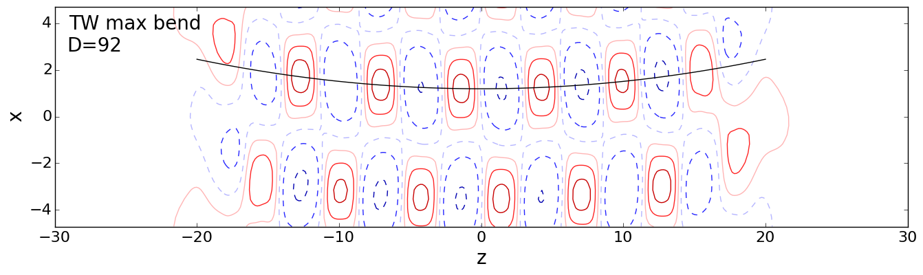
(c)
(d)

Figure 3: Bending and skewing. (color online) Contour plots of pressure $p(x,0,z)$ in the $y=0$ midplane are shown for localized equilibrium (EQ) and traveling-wave (TW) solutions with maximum and zero skewing and bending, corresponding to points marked on fig. 1(b). In (a,c), a line of constant slope passes through the pressure minima and maxima, showing uniformity of skew throughout the interior of the equilibrium solution, with (a) showing maximum skewing and (c) zero skewing. In (b,d), a line of constant curvature shows the uniformity of bending for the traveling wave, with (b) showing maximum bending and (d) zero bending. Eight contour levels are evenly spaced between $p=\pm 0.025$, dashed blue for negative $p$ and solid red for positive. The solution is shown for $L_{x}=3\pi$ and on a subset of the $L_{z}=16\pi$ computational domain.

Bending and skewing are most clearly illustrated in terms of the solution pressure fields for the points marked on the snaking curve of fig. 1(b). The interior structure of the equilibrium solution in fig. 3(a) is oriented along a diagonal line in the $x,z$ plane, whereas that of the traveling wave in fig. 3(b) curves upward in $x$ with increasing $z$. We call the former effect skewing and the latter bending. Skewing is an $x,z$-odd phenomenon associated with the $\sigma_{xyz}$ equilibrium symmetry (4), which gives an odd symmetry $p(x,z)=p(-x,-z)$ in the $y=0$ midplane. Similarly, bending is $x,z$-even and associated with the $\tau_{x}\sigma_{z}$ traveling-wave symmetry (5), which gives an even symmetry $p(x,z)=p(x+\ell_{x}/2,\,-z)$ in the midplane. We quantify skew or bending by the slope ($dx/dz$) or curvature ($d^{2}x/dz^{2}$) of an interpolating function that passes through the local minima and maxima of the midplane pressure field. Measured this way, bending and skewing are very nearly constant throughout the interior of any given solution, as illustrated by the lines of constant slope or curvature in fig. 3.

It is notable that the fronts of equilibrium and traveling-wave solutions are indistinguishable at maximum skew/bend (for example, the right-hand sides near $z\approx 20$ in fig. 3a,b) and also at zero skew/bend (fig. 3c,d). The fronts on the left-hand sides are determined from the right by symmetry. For the equilibrium, the odd $p(x,z)=p(-x,-z)$ symmetry means the $dx/dz$ slope of the structure has the same sign and magnitude at both the left and right fronts, so that the two fronts can be connected by a uniform periodic structure with constant slope. Importantly, the constant linear slope means the equilibrium solution can exist two steps higher up in $D$ (width) on the snaking curve, with the same internal winding structure and the same fronts, simply by adding more of the same interior periodic winding structure (or one step by adding half as much and flipping the solution with $\sigma_{z}$). The fact that the equilibrium solution can be extended in length this way with no change in interior structure thus explains why it snakes in a fixed region of Reynolds numbers, independently of $D$.

The even $p(x,z)=p(x+\ell_{x}/2,\,-z)$ symmetry of the traveling wave, on the other hand, means that the fronts impose a $dx/dz$ slope with opposite signs at the either end, so that the line connecting them generally must curve, as in fig. 3(b). We observe two features of this curvature in all localized traveling-wave solutions. First, the curvature is constant throughout the solution interior, so that the slope changes uniformly throughout. Thus in marked contrast to the equilibrium, the pattern on the interior of traveling wave is not periodic, but instead changes smoothly throughout. This is apparent in the changing relative streamwise phase of adjacent pressure minima and maxima of the traveling wave in fig. 3(b), but also more subtly in the long-$z$ modulation of the pressure field, which is visible through the changing magnitudes of the local maxima and minima of the pressure contours from one end of the solution to the other. Second, the slopes at the fronts vary between fixed bounds, the same bounds as for equilibria. Consequently, as the solution widens upwards along the snaking curve, the curvature decreases, and the interior structure becomes more periodic.

(a) (b)
(c) (d)

Figure 4: (a) Bending, (b) skewing, and (c) wave speed in comparison to (d) snaking in Reynolds number for the equilibrium (EQ), traveling-wave (TW), and rung (RN) solutions at $L_{x}=3\pi$ and a $L_{z}=24\pi$ computational domain. Dashed lines show the $~{}D^{-1}$ envelope of wave speed and bending for the traveling wave and the $D=\text{const}$ envelope of equilibrium skewing. In (a) two independent dashed lines of form $R+cD^{-1}$ are shown. The values of $R$ for the two lines were set as the lower and upper bounds of the equilibrium snaking curve ($R=236$ and $R=268$), and the values of $c$ chosen to fit the envelope of the traveling-wave snaking curve. Labeled points correspond to pressure fields shown in fig. 3.

Finite-size effects and $D^{-1}$ scaling. Fig. 4(a,b,c) show bending, skewing, and wave speed as a function of $D$, in comparison to the $\mathrm{Re},D$ snaking in fig. 4(d). Several features are notable. First, the solutions snake twice as fast in $\mathrm{Re}$ as in skewing, bending, or wave speed. This is due to the fact that the points of maximum magnitude in skewing and bending near the upper saddle-nodes in fig. 1(b) have opposite sign. Second, the traveling wave’s bending and streamwise wave speed curves are nearly identical (fig. 4a and c) in all aspects, including position of minima, maxima, and zeros, $D^{-1}$ scaling, and remarkably, magnitude. Sizable discrepancies between bending and wave speed occur only for $D<40$, when the traveling wave consists of only a few copies of the interior periodic pattern (e.g. fig. 2a,b). The nearly identical magnitudes of nondimensionalized bending and wave speed holds only for $L_{x}=3\pi$; at other $L_{x}$ the two quantities are strongly correlated but differ in magnitude by a factor of two or less.

Third, each of the traveling wave’s bending, wave speed, and $\mathrm{Re}$ snaking plots has a $D^{-1}$ envelope, whereas the corresponding plots for the equilibrium are constant in $D$. As argued above, the constancy of the equilibrium’s behaviour in $D$ is due to the fact that, with linear skew, the solution can be extended in $z$ and thus bumped up to a higher position on the snaking curve at the same Reynolds number simply by adding another copy of the periodic pattern in the interior. Thus the equilibrium snakes between constant bounds in Reynolds number and skewing. For the traveling wave, on the other hand, if we take the slope $dx/dz$ at the fronts as boundary conditions for constant interior curvature $d^{2}x/dz^{2}$ over a solution width that scales as $D$, then the curvature must scale as $D^{-1}dx/dz$. Given that the slope of the fronts oscillates between fixed bounds, the bending then must oscillate between bounds that scale as $D^{-1}$. For large $D$ the curvature thus approaches zero, and the interior of the solution approaches a constant periodic pattern with skewing, bending, and wave speed approaching zero.

At the point of zero bending (fig. 3d), the interior structure of the traveling wave is periodic and practically indistinguishable from the structure of the equilibrium at zero skew (fig. 3c). These points occur near low-$\mathrm{Re}$ saddle-node bifurcations (fig. 1b), suggesting that the reason for the close match in the lower bound in $\mathrm{Re}$ of the equilibrium and traveling-wave snaking regions is that the two solutions near the lower bifurcation point differ mainly in the orientation of one front. Lastly, the complete lack of symmetry in rung solutions means that they generally travel in $z$ as well as $x$; however, the nondimensionalized $z$ wave speeds are on the order of $10^{-5}$.

3.4 Core, front, tail structure

(a) (b)

Figure 5: Core, front, tails structure of the localized solutions. (a) Maximum magnitude of streamwise velocity ($\max_{xy}|u|$) and magnitude of mean streamwise velocity ($|\langle u\rangle_{xy}|$) as a function of $z$ for the traveling wave at a point of maximum bend ($\mathrm{Re}=275,D=48$). The $|\langle u\rangle_{xy}|$ line is dotted when $\langle u\rangle_{xy}$ is negative. (b) Magnitude of the $k_{x}$th streamwise Fourier mode for $k_{x}=0,1,2$, as measured by the root-mean-square magnitude of $\hat{{\bf u}}_{k_{x}}(y,z)$ over $y$ as a function of $z$. The computational domain is $3\pi\times 24\pi$ ($\alpha=2/3$).

The localized solutions are formed from nearly periodic, large-amplitude core structure surrounded by that taper into small-amplitude, exponentially decaying tails. The near periodicity of the core and the tapering fronts are apparent in fig. 2 and fig. 3. Fig. 5 illustrates the small-amplitude tails as well, through logarithmic plots of velocity magnitude as a function of the spanwise coordinate $z$. Fig. 5(a) shows $|\langle u\rangle_{xy}|(z)$, the magnitude of the $xy$-average streamwise flow, and $\max_{xy}|u|(z)$, the maximum over $x,y$ of the magnitude of the streamwise flow. Fig. 5(b) shows the root-mean-square magnitude over $y$ of several streamwise Fourier modes as a function of $z$. The central feature of these plots is the dominant $\exp(-\alpha|z|)$ scaling of the tails (where $\alpha=2\pi/L_{x}$), consistent with the the linear analysis presented in Gibson & Brand (2014). This analysis showed that for large $|z|$, the tails of spanwise-localized, streamwise-periodic solutions are dominated by the $k_{x}=\pm 1$ streamwise Fourier modes, which take the form $\hat{{\bf u}}_{\pm 1}(y)\exp{(\pm 2\pi\alpha i(x-c_{x}t)-\alpha|z|)}+c.c.$. The $\exp(-\alpha|z|)$ scaling of the $k_{x}=1$ mode is apparent in fig. 5(b). The magnitude of the streamwise velocity in the tails ($\max_{xy}|u|$) is dominated by the $k_{x}=\pm 1$ modes and thus has the same $\exp(-\alpha|z|)$ scaling, as shown in fig. 5(a). The $\exp(-2\alpha|z|)$ scaling of the $k_{x}=0$ Fourier mode in fig. 5(b) results from a resonance between the $k_{x}=\pm 1$ modes, which, when summed and substituted into the nonlinearity ${\bf u}\cdot{\bf\nabla}{\bf u}$, produce an $\exp(-2\alpha|z|)$ forcing term in the $k_{x}=0$ momentum equation. The $k_{x}=0$ Fourier mode carries the $xy$-average velocity, so $|\langle u\rangle_{xy}|$ in fig. 5(a) has $\exp(-2\alpha|z|)$ scaling, as well. The dominant $k_{x}=1$ mode thus produces a small, decaying, but non-zero and constant-sign mean streamwise velocity in the solution tails.

Figure 6: Net streamwise flow and wave speed of the traveling wave. The net streamwise flow $\bar{u}=(L_{x}L_{y})^{-1}\int_{xyz}u\,dx\,dy\,dz$ of the traveling wave at $L_{x}=3\pi$ varies between roughly fixed bounds, in comparison to the $D^{-1}$ scaling of the wave speed. Wave speed is magnified by a factor of twenty for visibility.

The mean streamwise flow $\langle u\rangle_{xy}(z)$ of the traveling wave has a number of interesting features due to its $z$-even symmetry, which results from the $\sigma_{z}\tau_{x}$ symmetry of the solution ${\bf u}$. For one, $\langle u\rangle_{xy}(z)$ has the same sign in both tails (positive for the solution depicted in fig. 5). Additionally, even $z$ symmetry allows for imbalance between positive and negative mean streamwise velocity when summed across the core and front regions. For example, there are three positive $\langle u\rangle_{xy}$ streaks and four negative large-magnitude streaks across the core and initial front of the traveling wave in fig. 5, flanked by two lower-magnitude positive streaks. Summing across the core and fronts, and the weak positive tails, gives a net negative streamwise flow across the entire computational domain. Thus we have, with zero pressure gradient conditions, a steady-state solution whose streamwise flow is net negative in the interior, net positive in the tails, and net negative over the whole flow domain. Fig. 6 shows how the net streamwise flow $\bar{u}=1/(L_{x}L_{y})\int_{xyz}u\,dx\,dy\,dz$ varies along the snaking curve (again, the lack of $L_{z}$ normalization provides for a measure of the deviation from laminar flow that is insensitive to the computational domain). Note that $\bar{u}$ varies between roughly fixed bounds as the solution width ($D$) increases, because it results from an $N$ versus $N+1$ imbalance of large-magnitude streamwise streaks of opposite sign. This is in contrast to wave speed and bending, which result from balances between the fixed-sized fronts and the increasing core and therefore scale as $D^{-1}$. For the localized equilibrium solution $\bar{u}$ is zero and the streamwise flows in the $\pm z$ tails have opposing sign, due to $\sigma_{xyz}$ symmetry of ${\bf u}$ and consequent odd symmetry in $\langle u\rangle_{xy}(z)$.

4 Effects of varying streamwise wavelength

4.1 Snaking region, skewing, and snaking breakdown

(a) (b)
(c) (d)

Figure 7: Snaking as a function of streamwise wavelength $L_{x}$. (a) Snaking curves for the equilibrium (EQ), traveling-wave (TW), and rung (RN) solutions at $L_{x}=2\pi,2.5\pi,3\pi,$ and $4\pi$. (b) Detail of snaking curve for $L_{x}=2.5\pi$. (c) Snaking breakdown for $L_{x}\geq 4.2\pi$. (d) Snaking breakdown for $L_{x}\leq 1.7\pi$.

In this section we examine the effects of changing the streamwise wavelength $L_{x}$. The central results are that snaking is robust in $L_{x}$ over the range $1.7\pi\leq L_{x}\leq 4.2\pi$ or $0.48\leq\alpha\leq 1.2$, and that the snaking region moves upward in Reynolds number with decreasing $L_{x}$, with snaking observed over the range $165\leq\mathrm{Re}\leq 2700$. Each of these bounds is reported to two digits accuracy. Thus the localized solutions and the homoclinic snaking behaviour occur over a wide range of Reynolds numbers, including the $\mathrm{Re}\approx 300$ to $400$ range where Barkley & Tuckerman (2005) and Duguet et al. (2009) observed laminar-turbulent patterns in plane Couette flow. Fig. 7(a) shows snaking curves for the localized solutions at a variety of streamwise wavelengths. The interlinked snaking structure of the equilibrium, traveling-wave, and rung solutions is preserved under variation in $L_{x}$ with the following trends. As $L_{x}$ decreases, the snaking region moves upwards in $\mathrm{Re}$ and widens. As in the $L_{x}=3\pi$ case, the width in $\mathrm{Re}$ of any given equilibrium snaking curve is constant in $D$, whereas the amplitude of the traveling-wave snaking region decays as $D^{-1}$. For $L_{x}=4\pi$ the excess amplitude of traveling-wave snaking region over the equilibrium is too small to be observed.

(a) (b)

Figure 8: Snaking region and maximum skewing as a function of wavelength. (a) The snaking region in $\mathrm{Re}$ as a function of $L_{x}$ for the localized equilibrium. The shaded region indicates the range of $\mathrm{Re}$ within which snaking occurs at a given $L_{x}$. (b) Maximum magnitude of skewing of the equilibrium solution as a function of $L_{x}$. For both figures, dots mark measured values, and the curves are interpolated.

Fig. 8(a) shows the snaking region of the localized equilibrium in Reynolds number as a function of the streamwise wavelength $L_{x}$. The boundaries of the snaking region in $\mathrm{Re}$ decrease roughly exponentially with $L_{x}$ for $L_{x}\leq 3\pi$. As $L_{x}$ increases to $4.2\pi$, the lower bound of the snaking region approaches a constant $\mathrm{Re}=165$. Snaking breaks down outside the range $1.7\pi\leq L_{x}\leq 4.2\pi$. Fig. 7(c,d) illustrates the manner of the snaking breakdown. Above and below this range, the solutions are unable to grow additional structure indefinitely at the fronts. Instead of snaking indefinitely, the solution curve turns around and continues to higher Reynolds numbers at roughly constant solution width. For $L_{x}$ values just beyond the given range, the solutions snake a few times before turning around, as illustrated by the $L_{x}=1.6\pi$ and $4.5\pi$ curves in Fig. 7(c,d).

It is notable that the breakdown of snaking at $L_{x}\approx 4\pi$ closely coincides with the vanishing of the amplitude of the $D^{-1}$ scaling in the traveling wave’s snaking region, as seen fig. 7(a). Similarly, the magnitudes of bending and skewing decrease with increasing $L_{x}$, and at $L_{x}\approx 4\pi$ are too small to be observed in plots of the velocity or pressure fields. Fig. 8(b) shows the magnitude of the oscillation in skewing over the snaking curve as a function of $L_{x}$, as measured by the slopes of the lines through pressure minima and maxima, as shown in fig. 3(b). It is possible that the breakdown of snaking for $L_{x}\gtrsim 4\pi$ is related to the disappearance of these effects at $L_{x}\approx 4\pi$.

Another defect in the homoclinic snaking scenario is shown in fig. 7(b). This detail of the snaking curves for $L_{x}=2.5\pi$ shows that the traveling wave solution has two distinct branches. The solid curve labeled “TW branch 1” was continued downward from high Reynolds numbers and small widths ($D\approx 7$) where it connects smoothly to the other snaking curves via continuation in $L_{x}$. However this solution branch does not snake; rather it turns around in a saddle-node bifurcation and continues back to at least $\mathrm{Re}=2000$ at finite width. In contrast the dashed curve labeled “TW branch 2” does snake upward in $D$; it constitutes the bulk of the $L_{x}=2.5\pi$ traveling wave snaking curve shown in fig. 7(a). The branch 2 traveling wave was obtained from the endpoint of the rung solution at $\mathrm{Re}\approx 360$, $D\approx 22$. We have observed similar defects in snaking curves at several other values of $L_{x}$ (not shown). It is possible that the snaking breakdown observed for $L_{x}<1.7\pi$ and $L_{x}>4.2\pi$ is of this type. That is, there might be branches of the solution curves for such $L_{x}$ that do snake but are disconnected from the solution curves pictured in fig. 7(c,d). Lastly, we note that snaking occurs when the solutions are continued in $L_{x}$ with $\mathrm{Re}$ fixed, within the shaded $\mathrm{Re},L_{x}$ parameter regions depicted in Fig. 8(a).

4.2 Stability

(a)    (b)

Figure 9: Instability of the localized equilibrium in relation to width and wavelength. The number of unstable eigenvalues of the localized equilibrium solution as a function of solution width ($D$), overlaid on the $\mathrm{Re},D$ snaking curve for (a) $L_{x}=4\pi$, (b) $L_{x}=3\pi$.

Fig. 6 shows the number of unstable eigenvalues of the $L_{x}=4\pi$ and $3\pi$ equilibrium solutions in comparison to their $\mathrm{Re},D$ snaking curves. At $L_{x}=3\pi$ the equilibrium has a minimum of two or three unstable eigenvalues at small spanwise width (low $D$). Thus it is not strictly an edge state of the flow (Skufca et al., 2006; Schneider & Eckhardt, 2006). However one of the corresponding unstable eigenfunctions is antisymmetric, making the solution an edge state of the flow when constrained to $\sigma_{xyz}$ symmetry. In both cases there is a general trend toward more unstable modes as the solution grows wider. The $L_{x}=3\pi$, $D\approx 100$ solutions depicted in fig. 3(a,c) have $O(20)$ unstable eigenvalues. Superimposed on this general trend is an oscillation in which the number of unstable eigenvalues increases and decreases along the snaking curve. For both cases the local maxima (minima) in the number of unstable modes occur at points of maximum (minimum) skewing magnitude. In other words, strongly skewed solutions are more unstable than solutions with weak or zero skew. The same trends occur at $L_{x}=2\pi$, with the smallest-width solution starting with six unstable eigenvalues. The trend towards more instabilities with increasing solution size contrasts with the Swift-Hohenberg equation, which shows no such growth. There is an oscillation in the instabilities of the one-dimensional cubic-quintic Swift-Hohenberg with each cycle along the snaking curve, between one and zero unstable eigenvalues (Burke & Knobloch, 2007).

5 The periodic pattern of the core

5.1 Relation of the periodic pattern to the NBCW solution

(a)
(b) (c) (d)

Figure 10: Extraction of the interior periodic pattern of a spanwise localized solution. (a) The spanwise-localized equilibrium at point of zero skew, $L_{x}=3\pi$, $D=47$, and $\mathrm{Re}=237$. Vertical lines at $z=\pm 2.85$ mark one copy of the nearly periodic interior structure. (b) An exact periodic equilibrium obtained by Newton-Krylov refinement of the structure extracted from (a), with $L_{x},L_{z}=3\pi,5.7$ and $\mathrm{Re}=237$. (c) The lower-branch NBCW equilibrium at the same parameter values as (b), obtained by continuation. Plotting conventions for (a,b,c) are the same as in fig. 2. (d) Bifurcation curves for the interior periodic pattern and the NBCW equilibrium for $L_{x}=2\pi,3\pi$ and $4\pi$ and aspect ratios $L_{x}/L_{z}=1.74,1.65,1.74$ respectively. The periodic interior pattern and lower-branch NBCW equilibrium shown in (b,c) are marked on the $L_{x}=3\pi$ curve with a circle and square respectively. The interior pattern extracted from spanwise-localized equilibrium at $L_{x}=2\pi$ and $4\pi$ are also marked with circles.

Schneider et al. (2010b) and Schneider et al. (2010a) established that the snaking solutions are closely related to the NBCW equilibria, in that they result from a localizing bifurcation of NBCW and resemble the structure of NBCW in their interior. However, the relationship between the core structure and the NBCW solutions is more complicated than previously supposed. In particular, for $L_{x}\leq 3\pi$, the interior pattern and the NBCW solution lie on distinct solution curves when continued in Reynolds number, although these curves can be connected by continuation in the higher-dimensional parameter space $L_{x},L_{z},\mathrm{Re}$.

To compare the interior pattern to the NBCW solution, we extracted one copy of the interior pattern of the equilibrium at a variety of $L_{x}$ values, as illustrated for $L_{x}=3\pi$ in fig. 10. We begin in fig. 10(a) with a streamwise-localized equilibrium solution at a point along the snaking curve of zero skew, in order to maximize the spanwise periodicity of the interior pattern. The natural spanwise wavelength $\hat{L}_{z}=5.70$ of the interior pattern was determined by finding the zeros of $\langle u\rangle_{xy}(z)$ on either side of $z=0$. In fig. 10(a) these points are marked with vertical lines at $z=\pm 2.85$. The nearly periodic interior pattern was then interpolated onto uniformly spaced grid points for a spanwise periodic computational domain of width $L_{z}=5.70$ and refined with a Newton-Krylov search to the exact equilibrium shown in fig. 10(b). We performed this operation to find the exact equilibrium solution corresponding to the interior periodic pattern at several streamwise wavelengths in the range $2\pi\leq L_{x}\leq 4\pi$. In each case the divergence and the Gibbs phenomenon of the interpolated field were small and the Newton-Krylov refinement converged quickly onto an exact equilibrium. The natural aspect ratio of the interior pattern was always found to be in the range $1.65\leq L_{x}/\hat{L}_{z}\leq 1.75$.

Fig. 10(d) shows bifurcation diagrams for the the NBCW solution and exact equilibrium computed from the interior pattern for $L_{x}=2\pi,3\pi$, and $4\pi$. Since these solutions are spanwise as well as streamwise periodic, we use the conventional measure of energy dissipation and wall shear rate

$$D_{tot}=I_{tot}=\frac{1}{2L_{x}L_{z}}\int_{-L_{x}/2}^{L_{x}/2}\int_{-L_{z}/2}^{L_{z}/2}\left.\frac{\partial u_{tot}}{\partial y}\right|_{y=-1}+\left.\frac{\partial u_{tot}}{\partial y}\right|_{y=1}dx\,dz.$$ (6)

The circles mark the $\mathrm{Re},D_{tot}$ positions of the interior-pattern equilibrium solutions computed from localized solutions as described above, and the lines indicate the parametric continuation of these solutions in $\mathrm{Re}$. For $L_{x}=4\pi$ it was straightforward to continue the NBCW solution to the same aspect ratio and Reynolds number and confirm that the pattern and the NBCW solution were the same. However, as $L_{x}$ decreases, the upper portion of the solution curve pinches off at a codimension-2 bifurcation point near $L_{x}=3\pi$, $\mathrm{Re}=237$, leaving the interior pattern and NBCW on distinct solution curves. This pinching occurs at an $L_{x}$ value just below the $L_{x}=3\pi$ solution curve shown in fig. 10(d). For $L_{x}=2\pi$, the solution curves for the interior pattern (dash-dot line marked with a circle) and the NBCW solution (dash-dot, no marker) are distinct.

5.2 A winding solution of plane Couette flow

Figure 11: A winding equilibrium solution of plane Couette flow at $\mathrm{Re}=268$. The solution is strictly periodic in $x$ but has $z$ periodicity involving a phase shift in $x$ of the form ${\bf u}(x,y,z+5.642)={\bf u}(x-0.496,y,z)$. Nineteen copies of the $3\pi\times 5.642$ pattern fit in the $3\pi\times 107.2$ periodic computational domain. Contours of the midplane pressure field $p(x,z)$ are shown with the same plotting conventions as fig. 3.

It is possible to compute a spatially periodic winding solution from a skewed localized equilibrium, that is, a solution with fundamental domain size $L_{x},\hat{L}_{z}$ that is strictly periodic in $x$, but whose $z$ periodicity involves a phase shift in $x$,

$${\bf u}(x,y,z+\hat{L}_{z})={\bf u}(x-\Delta x,y,z).$$ (7)

One such solution is illustrated in fig. 11. The solution was computed starting with a localized equilibrium with strong skewing, like that shown in fig. 3(a). An iterative process of continuation in the computational domain length $L_{z}$ and adjustment of skewing by continuation in Reynolds number was performed to find a localized equilibrium whose interior pattern divided the computational domain evenly ($L_{z}/\hat{L}_{z}\doteq N$) and whose skew precisely aligned with the $x,z$ diagonal of the computational domain. $N$ copies of this winding interior pattern were then interpolated onto the computational domain as shown in fig. 11 and refined with Newton-Krylov search. The resulting winding solution shown in fig. 11 at $\mathrm{Re}=268$ has a $L_{x}=3\pi,L_{z}=107.2$ computational domain and $N=19$, giving $\hat{L}_{z}=L_{z}/N\doteq 5.462$, $\Delta x=L_{x}/N\doteq 0.496$, and winding symmetry ${\bf u}(x,y,z+5.642)={\bf u}(x-0.496,y,z)$. The winding symmetry and ${\bf u}=\sigma_{xyz}{\bf u}$ were enforced during the Newton-Krylov search. It is likely that other winding solutions of shear flows could be computed without recourse to skewed localized solutions, simply by applying skewing coordinate transformations to known spatially periodic solutions and refining with Newton-Krylov search.

6 Conclusions

We have shown that homoclinic snaking is robust under changes in streamwise wavelength for the spanwise-localized solutions of plane Couette flow of Schneider et al. (2010a). Homoclinic snaking occurs for these solutions over streamwise wavelengths in the range $1.7\pi\leq L_{x}\leq 4.2\pi$ and Reynolds numbers $165\leq\mathrm{Re}\leq 2700$, and the snaking region moves upwards in $\mathrm{Re}$ as $L_{x}$ decreases. The localized equilibrium, traveling-wave, and rung solutions thus exist at arbitrarily large spanwise widths over a wide range of Reynolds numbers. Several new properties of the solutions become apparent as $L_{x}$ decreases below $4\pi$, most importantly the linear skewing of the equilibrium and quadratic bending of the traveling wave. The traveling wave exhibits finite-size effects such as $D^{-1}$ scaling of the bending, wavespeed, and snaking region, due to the nonuniform structure in the solution core induced by the quadratic bending. The linear skewing of the localized equilibrium solution, on the other hand, induces no such finite-size effects. Its core region is very nearly periodic, close enough that a strictly periodic winding solution can be easily developed from it. The number of instabilities of the localized solutions increase with Reynolds number, with width, and with skewing. Thus, at a fixed Reynolds number, from a statistical viewpoint one would expect narrow patches of the localized pattern to appear more frequently than wide patches, and with weak rather than strong skewing.

The homoclinic snaking of these localized solutions suggests the Navier-Stokes equations might be related to the Swift-Hohenberg equation under plane Couette flow conditions and for certain parameter ranges and flow states. A primary motivation for this paper is to clarify the parameter ranges and solution structures for which this connection might occur. Our results indicate that homoclinic snaking is a finite-Reynolds, finite-wavelength effect, and that the streamwise wavelength and the Reynolds-number snaking region are strongly coupled. Thus it is unlikely that an analytic understanding of homoclinic snaking in shear flows will be found via asymptotic analysis in large-Reynolds or large-wavelength limits. If the spanwise-localized solutions are to be understood as a long-wavelength modulation of a small-wavelength, spanwise-periodic pattern, our results show that the periodic pattern is a form of the NBCW solution at aspect ratio $L_{x}/L_{z}\approx 1.7$. For $L_{x}<3\pi$, under continuation in Reynolds number, the periodic pattern lies on a solution curve distinct from the widely-studied NBCW lower-branch solution.

We see no clear connection between the skewing of the localized equilibrium solution and the skewed laminar-turbulent patterns observed in plane Couette flow by Barkley & Tuckerman (2005) and Duguet et al. (2009). The localized solutions exists over a much wider range of Reynolds numbers than the $300\leq\mathrm{Re}\leq 400$ range of the observed laminar-turbulent patterns. Also, the skewing of the localized equilibrium is a streamwise phase shift of the interior pattern as function of spanwise coordinate, whereas the skewing of observed laminar-turbulent patterns is in the orientation of the boundary between turbulent patches and surrounding laminar flow. The localized solutions studied here are strictly streamwise periodic, and thus have laminar-turbulent boundaries aligned with the streamwise direction. One potential route to finding invariant solutions with skewed laminar-nonlaminar boundaries would be to find a streamwise-localized form of a winding solution like that described § 5.2. However, the skewing observed in laminar-turbulent patterns is much larger than any observed here. Duguet et al. (2010) reports that the boundaries of turbulent patches in $\mathrm{Re}\approx 300$ plane Couette flow lie within the range of angles $\beta=36^{\circ}\pm 10^{\circ}$ off the streamwise axis. This corresponds to range of skewing slopes $dx/dz=\tan(90^{\circ}-\beta)$ between roughly 1 and 2, much larger than the maximum skew of $dx/dz\approx 0.1$ of the equilibria in the parameter range $\mathrm{Re}\approx 300$, $2.75\pi<L_{x}<3\pi$.

Acknowledgements: The authors thank John Burke and Edgar Knobloch for illuminating conversations, and John Burke for assistance in the numerical calculations. TMS was supported by the Swiss National Science Foundation under grant number 200021-160088. Computations were performed on Trillian, a Cray XE6m-200 supercomputer at the University of New Hampshire supported by the Major Research Instrumentation program of the United States National Science Foundation under grant PHY-1229408.

References

- Avila et al. (2013) Avila, M., Mellibovsky, F., Roland, N. & Hof, B. 2013 Streamwise-localized solutions at the onset of turbulence in pipe flow. Phys. Rev. Lett. 110, 224502.
- Barkley & Tuckerman (2005) Barkley, D. & Tuckerman, L. S. 2005 Computational study of turbulent laminar patterns in Couette flow. Phys. Rev. Lett. 94, 014502.
- Batiste & Knobloch (2005) Batiste, O. & Knobloch, E. 2005 Simulations of localized states of stationary convection in He-3-He-4 mixtures. Phys. Rev. Lett. 95 (24), 244501.
- Batiste et al. (2006) Batiste, O., Knobloch, E., Alonso, A. & Mercader, I. 2006 Spatially localized binary-fluid convection. J. Fluid Mech 560, 149–158.
- Beaume et al. (2015) Beaume, C., Chini, G. P., Julien, K. & Knobloch, E. 2015 Reduced description of exact coherent states in parallel shear flows. Phys. Rev. E 91 (4), 043010.
- Beck et al. (2009) Beck, M., Knobloch, J., Lloyd, D., Sandstede, B. & Wagenknecht, T. 2009 Snakes, ladders, and isolas of localized patterns. SIAM J. Math. Anal. 41, 936–972.
- Brand & Gibson (2014) Brand, E. & Gibson, J. F. 2014 A doubly-localized equilibrium solution of plane Couette flow. J. Fluid Mech. 750 (R3), 1–12.
- Burke & Knobloch (2007) Burke, J. & Knobloch, E. 2007 Homoclinic snaking: structure and stability. Chaos: An Interdisciplinary Journal of Nonlinear Science 17 (3), 037102.
- Chantry et al. (2014) Chantry, M., Willis, A. P. & Kerswell, R. R. 2014 Genesis of streamwise-localized solutions from globally periodic traveling waves in pipe flow. Phys. Rev. Lett. 112 (16), 164501.
- Clever & Busse (1997) Clever, R. & Busse, F. 1997 Tertiary and quaternary solutions for plane Couette flow. J. Fluid Mech. 344, 137–153.
- Deguchi et al. (2013) Deguchi, K., Hall, P. & Walton, A. 2013 The emergence of localized vortex-wave interaction states in plane Couette flow. J. Fluid Mech. 721, 58–85.
- Duguet et al. (2008) Duguet, Y., Pringle, C. & Kerswell, R. 2008 Relative periodic orbits in transitional pipe flow. Phys. Fluids 20, 114102.
- Duguet et al. (2010) Duguet, Y., Schlatter, P. & Henningson, D. 2010 Formation of turbulent patterns near the onset of transition in plane Couette flow. J. Fluid Mech. 650, 119–129.
- Duguet et al. (2009) Duguet, Y., Schlatter, P. & Henningson, D. S. 2009 Localized edge states in plane Couette flow. Phys. Fluids 21, 111701.
- Dummit & Foote (2004) Dummit, D. & Foote, R. 2004 Abstract Algebra. Hoboken, NJ: John Wiley & Sons.
- Faisst & Eckhardt (2003) Faisst, H. & Eckhardt, B. 2003 Traveling waves in pipe flow. Phys. Rev. Lett. 91, 224502.
- Gibson & Brand (2014) Gibson, J. F. & Brand, E. 2014 Spatially localized solutions of planar shear flow. J. Fluid Mech. 745, 25–61.
- Gibson et al. (2008) Gibson, J. F., Halcrow, J. & Cvitanović, P. 2008 Visualizing the geometry of state space in plane Couette flow. J. Fluid Mech. 611, 107–130.
- Gibson et al. (2009) Gibson, J. F., Halcrow, J. & Cvitanović, P. 2009 Equilibrium and traveling-wave solutions of plane Couette flow. J. Fluid Mech. 638, 1–24.
- Hall (2012) Hall, P. 2012 Vortex–wave interactions: long-wavelength streaks and spatial localization in natural convection. J. Fluid Mech. 703, 99–110.
- Hall & Sherwin (2010) Hall, P. & Sherwin, S. 2010 Streamwise vortices in shear flows: harbingers of transition and the skeleton of coherent structures. J. Fluid Mech. 661, 178–205.
- Jiménez & Moin (1991) Jiménez, J. & Moin, P. 1991 The minimal flow unit in near-wall turbulence. J. Fluid Mech. 225, 213–240.
- Kawahara & Kida (2001) Kawahara, G. & Kida, S. 2001 Periodic motion embedded in plane Couette turbulence: regeneration cycle and burst. J. Fluid Mech. 449, 291–300.
- Kawahara et al. (2012) Kawahara, G., Uhlmann, M. & van Veen, L. 2012 The significance of simple invariant solutions in turbulent flows. Ann. Rev. Fluid Mech. 44, 203–225.
- Knobloch (2015) Knobloch, E. 2015 Spatial localization in dissipative systems. Ann. Rev. Condens. Matter Phys. 6, 325–359.
- Mellibovsky & Meseguer (2015) Mellibovsky, F. & Meseguer, A. 2015 A mechanism for localization of nonlinear waves in shear flows. J. Fluid Mech. 779 (R3), 1–11.
- Nagata (1990) Nagata, M. 1990 Three-dimensional finite-amplitude solutions in plane Couette flow: bifurcation from infinity. J. Fluid Mech. 217, 519–527.
- Schneider & Eckhardt (2006) Schneider, T. M. & Eckhardt, B. 2006 Edge of chaos in pipe flow. Chaos: An Interdisciplinary Journal of Nonlinear Science 16 (4), 041103.
- Schneider et al. (2010a) Schneider, T. M., Gibson, J. F. & Burke, J. 2010a Snakes and ladders: Localized solutions of plane Couette flow. Phys. Rev. Lett. 104, 104501.
- Schneider et al. (2010b) Schneider, T. M., Marinc, D. & Eckhardt, B. 2010b Localised edge states nucleate turbulence in extended plane Couette cells. J. Fluid Mech. 646, 441–451.
- Skufca et al. (2006) Skufca, J., Yorke, J. & Eckhardt, B. 2006 The edge of chaos in a parallel shear flow. Phys. Rev. Lett. 96, 174101.
- Tuckerman et al. (2014) Tuckerman, L., Kreilos, T., Schrobsdorff, H., Schneider, T. & Gibson, J. 2014 Turbulent-laminar patterns in plane Poiseuille flow. Phys. Fluids 26, 114103.
- Viswanath (2007) Viswanath, D. 2007 Recurrent motions within plane Couette turbulence. J. Fluid Mech. 580, 339–358.
- Waleffe (1998) Waleffe, F. 1998 Three-dimensional coherent states in plane shear flows. Phys. Rev. Lett. 81, 4140–4143.
- Waleffe (2001) Waleffe, F. 2001 Exact coherent structures in channel flow. J. Fluid Mech. 435, 93–102.
- Waleffe (2003) Waleffe, F. 2003 Homotopy of exact coherent structures in plane shear flows. Phys. Fluids 15, 1517–1534.
- Wedin & Kerswell (2004) Wedin, H. & Kerswell, R. R. 2004 Exact coherent structures in pipe flow: traveling wave solutions. J. Fluid Mech. 508, 333–371.
- Zammert & Eckhardt (2014a) Zammert, S. & Eckhardt, B. 2014a Periodically bursting edge states in plane Poiseuille flow. Fluid Dynamics Research 46 (4), 041419.
- Zammert & Eckhardt (2014b) Zammert, S. & Eckhardt, B. 2014b Streamwise and doubly-localised periodic orbits in plane Poiseuille flow. J. Fluid Mech. 761, 348–359.