Higher-order Hamiltonian Model for Unidirectional Water Waves

Abstract.

Formally second-order correct, mathematical descriptions of long-crested water waves propagating mainly in one direction are derived. These equations are analogous to the first-order approximations of KdV- or BBM-type. The advantage of these more complex equations is that their solutions corresponding to physically relevant initial perturbations of the rest state may be accurate on a much longer time scale. The initial-value problem for the class of equations that emerges from our derivation is then considered. A local well-posedness theory is straightforwardly established by way of a contraction mapping argument. A subclass of these equations possess a special Hamiltonian structure that implies the local theory can be continued indefinitely.

1. Introduction

Long-crested water waves propagating shoreward are commonplace in the shallow water zone of large bodies of water. Waves of this general form are easily generated in laboratory settings as well. If a standard $xyz$–coordinate system is adopted in which $z$ increases in the direction opposite to which gravity acts, such waves are often taken to propagate along the $x$–axis, say in the direction of increasing values, and to be independent of the $y$-coordinate. In this case, if dissipation and surface tension effects are ignored, the fluid assumed to be incompressible and the motion irrotational, the standard representation of the velocity field and the free surface is provided by the Euler equations for the motion of a perfect fluid with the boundary behavior at the free surface determined by the Bernoulli condition. On typical geophysical length scales, these equations provide reasonably good approximations of what is actually observed in nature. In detail, this system has the form

$$\begin{cases}\Delta{\varphi}=0,\qquad\qquad&0<y<h_{0}+\eta(x,t),\\ \partial_{y}\varphi=0,&y=0,\\ \partial_{t}\eta=\partial_{y}\varphi-\partial_{x}{\eta}\cdot\partial_{x}{\varphi},&y=h_{0}+\eta(x,t),\\ ‎\partial_{t}\varphi=g\eta-\frac{1}{2}(\partial_{x}\varphi)^{2}-\frac{1}{2}(\partial_{y}\varphi)^{2},&y=h_{0}+\eta(x,t).\end{cases}$$ (1.1)

Here, the bottom is taken to be flat, horizontal and located at $z=0$, though theory with a slowly varying bottom can easily be derived along the same lines (see [15]). The undisturbed depth is $h_{0}$ while the dependent variable, $\eta=\eta(x,t)$ is the deviation of the free surface from its rest position $(x,h_{0})$ at time $t$. Thus, the depth of the water column over the spatial point $(x,0)$ on the bottom, at time $t$ is $h(x,t)=h_{0}+\eta(x,t)$. The dependent variable $\phi=\phi(x,y,t)$ is the velocity potential which is defined throughout the flow domain, and whose existence owes to the fact that the fluid is incompressible and irrotational. Hence, $(u(x,z,t),v(x,z,t))=\nabla\phi(x,z,t)$ is the velocity field at the point $(x,z)$ in the flow domain at time $t$. Here, $\nabla$ connotes the gradient with respect to the spatial variables only. Of course, for this formulation to make sense, it must be the case that the free surface remains a graph over the bottom, a presumption that overlies the developments here. It deserves remark that the system (1.1) can be rewritten in a Hamiltonian form, as Zakharov [50] pointed out almost 50 years ago.

Beginning already in the first half of the $19^{th}$–century, simpler models have been posited, in part because the approximation using (1.1) is both analytically and computationally recalcitrant. Note in particular that the location of the free surface is part of the problem, so that two boundary conditions at the free surface are needed for its determination. Observe also that the temporal derivatives only appear in the boundary conditions, making the problem further non-standard. Moreover, the precision one might hope for from using the Euler equations is not always needed in practice. If the input data has significant error, there may be little point in the higher accuracy afforded by the Euler system (1.1) as opposed to cruder approximations.

The largest steps forward in the $19^{th}$ century study of approximate models were taken by Boussinesq in the 1870’s (see especially his opus [27]). The coupled systems of equations which now bear his name are well known to theoreticians and they and their relatives find frequent use in practical situations (see, e.g. [8], [15]). In addition to the presumption that the wave motion is long-crested, so sensibly one-dimensional, they subsist on the assumption that the wave amplitudes and wavelengths encountered in the evolution are, respectively, small and large relative to the undisturbed depth $h_{0}$ of the liquid over the horizontal, featureless bottom. More precisely, their derivation needs that

$$\alpha=\frac{A}{h_{0}}\ll 1,\qquad\beta=\frac{h_{0}^{2}}{l^{2}}\ll 1,\qquad S=\frac{\alpha}{\beta}=\frac{Al^{2}}{h_{0}^{3}}\approx 1.$$ (1.2)

Here, $A$ is a typical amplitude of the wave motion in question while $l$ is a typical wavelength. The assumption that the Stokes’ number $S=\frac{\alpha}{\beta}$ is of order one effectively means that nonlinear and dispersive effects are balanced. Boussinesq also derived a model, now called the Korteweg–de Vries (KdV) equation, which was a specialization of the coupled systems, formally valid for waves traveling only in one direction, say in the direction of increasing values of $x$.

Almost a century later, Peregrine [45] and Benjamin et al. [7] returned to Boussinesq’s unidirectional model

$$\eta_{t}+\eta_{x}+\frac{3}{2}\eta\eta_{x}+\frac{1}{6}\eta_{xxx}=0$$ (1.3)

(the Korteweg-de Vries equation, commonly referred to as the KdV equation) and derived an equivalent version known as the regularized long-wave equation (RLW-equation) or the BBM-equation. In terms of the dependent variable $\eta(x,t)$, this equation takes the form

$$\eta_{t}+\eta_{x}+\frac{3}{2}\eta\eta_{x}-\frac{1}{6}\eta_{xxt}=0$$ (1.4)

in the unscaled, non-dimensional variables

$$x=\frac{1}{h_{0}}\,\bar{x},\quad t=\sqrt{\frac{g}{h_{0}}}\,\bar{t}\quad{\rm and}\quad\eta=\frac{1}{h_{0}}\,\bar{\eta}.$$

Here, the constant $g$ is the acceleration due to gravity while $\bar{x},\bar{t}$ and $\bar{\eta}$ are laboratory or field variables, all measured in the unit of length consistent with the values of $h_{0}$ and $g$.

Models like the BBM- and KdV-equation are known to provide good approximations of unidirectional solutions of the full water wave problem (1.1) on the so-called Boussinesq time scale, $\frac{1}{\beta}\approx\frac{1}{\alpha}$ (see [2], [18], [21]). They are also known to predict laboratory observations with reasonable accuracy on similar time scales (see [20], [35], [36]).

In some applications, notably coastal engineering and ocean wave modeling, the waves need to be followed on time scales longer than the Boussinesq time scale (for example, see [8] and references therein). In such situations, a higher-order approximation to the water-wave problem might prove to be useful as it would be formally valid on the square $\frac{1}{\beta^{2}}\approx\frac{1}{\alpha^{2}}$ of the long, Boussinesq time scale. Such models have appeared in the literature before (see [43, 44] for early examples). It is our purpose here to put forward a class of such higher-order correct, unidirectional evolution equations and to provide analysis relating to the fundamental issue of Hadamard well-posedness for a subclass. Models will be isolated that are not only a formally second-order correct approximation of the full, two-dimensional water wave problem, but also possesses a Hamiltonian structure. As P. Olver pointed out in his pioneering work [44], this helpful aspect is more difficult to attain in higher-order models that formally are faithful to the overlying Euler equations than in the first-order correct KdV or BBM models. Indeed, the fifth-order model appearing in [44] does not in fact have a Hamiltonian structure, as Olver points out.

The notion of well-posedness which is featured here was put forward by Hadamard more than a century ago in a lecture the well known French mathematician gave at Princeton University (see [34]). In his conception, a problem is well-posed subject to given auxiliary data when there corresponds a unique solution which depends continuously on variations in the specified supplementary data. Hadamard points out that if the problem is lacking these properties, it will probably be useless in practical applications. Auxiliary data brought from real world situations typically features at least a small amount of error. If the model were to respond discontinuously to these small perturbations, the reproducibility of the model predictions in laboratory and field settings would be compromised and likewise their use in real situations would be suspect.

To clarify the role of the size restrictions (1.2), it is often helpful to rescale the variables. For example, in the context of equation (1.4), change variables by letting $\eta\hookrightarrow\alpha\eta$, and $(x,t)\hookrightarrow\sqrt{\beta}(x,t)$. In the new variables, $\eta$ and its first few partial derivatives with respect to $x$ and $t$ are presumed to be of order one and the equation takes the form

$$\eta_{t}+\eta_{x}+\frac{3}{2}\alpha\eta\eta_{x}-\frac{1}{6}\beta\eta_{xxt}=0.$$ (1.5)

In this scaling, the role of the small parameters is more apparent. Moreover, the error term made in the approximation, which is set to zero in (1.5), is quadratic in the small parameters $\alpha$ and $\beta$. Because of this latter aspect, even though the solution and its derivatives remains of order one, the ignored error can accumulate and have an order-one effect on the solution on a time scale of size $\frac{1}{\alpha^{2}}\approx\frac{1}{\beta^{2}}$, hence the need for a higher-order correct model if longer spatial distances are in question.

The starting point of our derivation of higher-order KdV-BBM-type equations is the paper [12] (and see also the earlier note [15]) where a several-parameter variant of the classical Boussinesq system of two coupled equations was derived. These Boussinesq systems are derived without the assumption of one-way propagation and can therefore countenance long-crested waves propagating in both directions. The theory in [12] assumes incompressibility, irrotationality, long-crestedness and the size conditions enunciated in (1.2). Boussinesq systems were formally derived at both first and second order in the small parameters $\alpha$ and $\beta$. In dimensionless, scaled variables as appearing in (1.5), the family of formally first-order correct systems has the form

$$\begin{cases}\eta_{t}+w_{x}+\alpha(w\eta)_{x}+\beta\big{(}aw_{xxx}-b\eta_{xxt}\big{)}=0,\\ w_{t}+\eta_{x}+\alpha ww_{x}+\beta\big{(}c\eta_{xxx}-dw_{xxt}\big{)}=0.\end{cases}$$ (1.6)

The variable $\eta$ is proportional to the deviation of the free surface from its rest position at the point $x$ at time $t$, as it was in (1.4), while $w=w(x,t)$ is proportional to the horizontal velocity at a certain depth $z_{0}$, say, at the point $(x,z_{0},t)$ in the flow domain. (The velocity $w$ is scaled by $\sqrt{gh_{0}}$ to make it non-dimensional, and then by $\alpha$ to make it of order one.) The constants $a,b,c$ and $d$ are not arbitrary. They satisfy the relations

$$\begin{cases}a=\frac{1}{2}\Big{(}\theta^{2}-\frac{1}{3}\Big{)}\lambda,\qquad&b=\frac{1}{2}\Big{(}\theta^{2}-\frac{1}{3}\Big{)}(1-\lambda),\\ c=\frac{1}{2}(1-\theta^{2})\mu,\qquad\quad&d=\frac{1}{2}(1-\theta^{2})(1-\mu),\end{cases}$$ (1.7)

so that $a+b+c+d=\frac{1}{3}$. In the same, order-one, independent and dependent variables, the second-order correct systems are

$$\begin{cases}\begin{split}\eta_{t}&+w_{x}+\beta\big{(}aw_{xxx}-b\eta_{xxt}\big{)}+\beta^{2}\big{(}a_{1}w_{xxxxx}+b_{1}\eta_{xxxxt}\big{)}\\ &=-\alpha(\eta w)_{x}+\alpha\beta\big{(}b(\eta w)_{xxx}-(a+b-\frac{1}{3})(\eta w_{xx})_{x}\big{)},\\ w_{t}&+\eta_{x}+\beta\big{(}c\eta_{xxx}-dw_{xxt}\big{)}+\beta^{2}\big{(}c_{1}\eta_{xxxxx}+d_{1}w_{xxxxt}\big{)}\\ &=-\alpha ww_{x}\!+\!\alpha\beta\big{(}(\!c\!+\!d)ww_{xxx}\!-\!c(ww_{x})_{xx}-\!(\eta\eta_{xx})_{x}\!+\!(\!c\!+\!d\!-\!1\!)w_{x}w_{xx}\big{)},\end{split}\end{cases}$$ (1.8)

where the additional constants $a_{1},b_{1},c_{1},d_{1}$ are

$$\begin{cases}\begin{split}a_{1}&=-\frac{1}{4}\Big{(}\theta^{2}-\frac{1}{3}\Big{)}^{2}(1-\lambda)+\frac{5}{24}\Big{(}\theta^{2}-\frac{1}{5}\Big{)}^{2}\lambda_{1},\\ b_{1}&=-\frac{5}{24}\Big{(}\theta^{2}-\frac{1}{5}\Big{)}^{2}(1-\lambda_{1}),\\ c_{1}&=\frac{5}{24}(1-\theta^{2})\Big{(}\theta^{2}-\frac{1}{5}\Big{)}(1-\mu_{1}),\\ d_{1}&=-\frac{1}{4}\big{(}1-\theta^{2}\big{)}^{2}\mu-\frac{5}{24}(1-\theta^{2})\Big{(}\theta^{2}-\frac{1}{5}\Big{)}\mu_{1}.\end{split}\end{cases}$$ (1.9)

The parameter $\theta$ has physical significance. It is determined by the height above the bottom at which the horizontal velocity is specified initially and whose evolution is being followed. In the earlier notation, $\theta=1-z_{0}$. Because the vertical variable is scaled by the undisturbed depth $h_{0}$ in these descriptions, $\theta$ must lie in the interval $[0,1]$. The other values, $\lambda,\mu,\lambda_{1}$ and $\mu_{1}$ are modeling parameters and can in principle take any real value. Thus the coefficients appearing in the higher-order Boussinesq systems form a restricted, eight-parameter family. Notice that if terms quadratic in $\alpha$ and $\beta$ are dropped, the second-order system (1.8) reduces to the first-order system (1.6).

The velocity field in the rest of the flow is determined by an associated approximation of the velocity potential in the flow-domain. The latter is derived from a knowledge of $w$ (see [12], [17]).

Local in time well-posedness of the Cauchy problem for the systems (1.6) and (1.8) was studied in [12] and [13]. Not all of these systems are even linearly well-posed. Indeed, the recent foray [5] shows that many of those not linearly well-posed are in fact not locally well-posed when the nonlinearity is taken into account. The fact that some of the family is ill-posed has the advantage of eliminating them from consideration when real-world approximation is the goal.

These systems were further extended in [18] to include waves that are fully three-dimensional, and not just long-crested motions. Rigorous estimates were also provided for the difference between solutions of the full water-wave problem and solutions of the first-order models. A further extension of [18] is given in [39], where Boussinesq systems in the Kadomtsev-Petviashvili (KP) scaling are derived. The latter situation is intermediate between the long-crested regime where transverse motion is ignored entirely and three-dimensional Boussinesq systems that allow strong transverse disturbance; a regime that is often referred to as allowing for weakly transverse long waves. A detailed survey of results of this sort can be found in J.-C. Saut’s lecture notes [46] or the recent monograph of Lannes [38].

As hinted already, when long-crested waves are essentially moving in only one direction, one might prefer to use a unidirectional model because less auxiliary data is needed to initiate it. Theory developed in [2] has shown rigorously that predictions of first-order Boussinesq systems and those of their unidirectional counterpart (1.4) are the same to the neglected order, provided the wave motion is initiated unidirectionally. This gives rigorous credence to the utility of such unidirectional models since the bidirectional models are known to be a good approximation of solutions of the full Euler system in the Boussinesq regime of small amplitude and long wavelength.

We stress that while the higher-order, unidirectional models put forward here are formally correct on the square of the Boussinesq time scale, no proof of this exists. Indeed, considering the difficulty encountered in showing the first-order correct, Boussinesq systems are faithful to the full, inviscid water wave problem (1.1) on the Boussinesq time scale and showing the KdV-BBM approximations (1.3)-(1.4) is true to their overlying Boussinesq system, a rigorous result for the systems derived here on the square of the Boussinesq time scale is likely to be challenging. One can show that the higher-order terms do not do damage to the original KdV-BBM approximation of the full water-wave problem on the Boussinesq time scale, provided sufficiently smooth initial data are countenanced. This point is not addressed here as it would take us afield of the main developments. It is also the case that one can show directly and rigorously that the linearized, higher-order, unidirectional model is faithful to the linearized Boussinsq system on this very long time scale, again, provided the initial data has enough regularity. However, these results are far from what one would like to have in hand.

The present contribution proceeds as follows. In the next section, we derive formally from the second-order Boussinesq equations a class of second-order KdV-BBM-type equations. Also in the next section, function class notation is introduced and our main results about the higher-order, unidirectional models are stated. Section 3 provides proofs of the results stated in Section 2.2, while Section 4 features commentary about the choice of the parameters $\theta,\lambda,\mu,\lambda_{1}$, $\mu_{1}$ and another parameter $\rho$ to be introduced presently. Section 5 is devoted to a discussion of the linear dispersion relation. Finally, in Section 6 some concluding remarks are recorded.

2. Derivation of the Models and the Main Results

The formal derivation of a class of higher-order, unidirectional equations, together with a precise statement of results about their well-posedness is the topic of this section.

2.1. Model Equations

The starting point is the collection (1.8) of higher-order Boussinesq systems derived in [12]. The parameters $a,b,\cdots c_{1},d_{1}$ are those presented in (1.7) and (1.9). As we are working in the Boussinesq regime where the Stokes’ number $S=\frac{\alpha}{\beta}\approx 1$, the two small parameters $\alpha$ and $\beta$ are treated on an equal footing. Thus, $O(\alpha)=O(\beta),\,O(\alpha\beta)=O(\beta^{2})$, etc.

In case the wave motion is essentially in one direction, say in the direction of increasing values of $x$, we will show how to reduce such Boussinesq systems to the single, fifth-order model,

$$\begin{split}\eta_{t}+\eta_{x}-\beta\gamma_{1}\eta_{xxt}+&\beta\gamma_{2}\eta_{xxx}+\beta^{2}\delta_{1}\eta_{xxxxt}+\beta^{2}\delta_{2}\eta_{xxxxx}+\alpha\frac{3}{4}(\eta^{2})_{x}\\ &+\,\alpha\beta\Big{(}\gamma(\eta^{2})_{xxx}-\frac{7}{48}(\eta_{x}^{2})_{x}\Big{)}-\alpha^{2}\frac{1}{8}(\eta^{3})_{x}=0.\end{split}$$ (2.10)

The constants $\gamma_{1}$, $\gamma_{2}$, $\delta_{1}$, $\delta_{2}$ and $\gamma$ depend upon the parameters $a,b,\cdots$ in (1.8) and will be displayed presently.

Passage from the Boussinesq systems (1.8) to the unidirectional models (2.10) follows the same line of argument as did the passage from the first-order system (1.6) to the mixed KdV–BBM equations

$$\eta_{t}+\eta_{x}+\frac{3}{2}\alpha\eta\eta_{x}+\nu\beta\eta_{xxx}-\Big{(}\frac{1}{6}-\nu\Big{)}\beta\eta_{xxt}\,=\,0,$$ (2.11)

where $\nu=\frac{1}{2}(a+c)=\frac{1}{4}\big{[}\theta^{2}(\lambda-\mu)-\frac{1}{3}\lambda+\mu\big{]}$ depends upon $\theta,\lambda$ and $\mu$ and can formally take any real value. (See [2], [29] and, in the internal wave context, [30]. A special case of this model may be found in [25] for a moving boundary problem.)

As described in [9], at the lowest order of approximation wherein the parameters are small enough that even the first-order terms in $\alpha$ and $\beta$ may be dropped, the system (1.8) becomes the one-dimensional wave equation, viz.

$$\begin{cases}\eta_{t}+w_{x}=0,\qquad\quad w_{t}+\eta_{x}=0,\\ \eta(x,0)=f(x),\qquad w(x,0)=g(x),\end{cases}$$ (2.12)

where $f(x)$ and $g(x)$ are the initial disturbances of the surface and the horizontal velocity, respectively. The solution to (2.12) is

$$\begin{cases}\begin{split}\eta(x,t)=\frac{1}{2}\big{[}f(x+t)+f(x-t)\big{]}-\frac{1}{2}\big{[}g(x+t)-g(x-t)\big{]},\\ w(x,t)=\frac{1}{2}\big{[}g(x+t)+g(x-t)\big{]}-\frac{1}{2}\big{[}f(x+t)-f(x-t)\big{]}.\end{split}\end{cases}$$ (2.13)

For the left-propagating component to vanish, one must have $f=g$, in which case $\eta(x,t)=f(x-t)$,

$$\eta_{t}+\eta_{x}=0\quad{\rm and}\quad w=\eta.$$

Notice in particular that in the Boussinesq regime, when most of the propagation is to the right, it appears that

$$\eta_{t}=-\eta_{x}+O(\alpha,\beta),\quad{\textrm{as}}\quad\alpha,\beta\to 0,$$ (2.14)

a point that will play a significant role in what follows.

At the next order when one keeps terms of first order in $\alpha$ and $\beta$, the standard ansatz used in [2] was that

$$w=\eta+\alpha A+\beta B$$ (2.15)

where $A=A(\eta,\cdots)$ and $B=B(\eta_{xx},\eta_{xt},\cdots)$ turn out to be simple polynomial functions of $\eta$ and its first few partial derivatives. Indeed, substituting (2.15) into the first-order system (1.6) and dropping all terms of quadratic order in the small parameters $\alpha$ and $\beta$ leads to the pair

$$\begin{cases}\begin{split}\eta_{t}+\eta_{x}+\alpha A_{x}+\beta B_{x}+\alpha(\eta^{2})_{x}+\beta\big{(}a\eta_{xxx}-b\eta_{xxt}\big{)}\,=\,0,\\ \eta_{t}+\alpha A_{t}+\beta B_{t}+\eta_{x}+\alpha ww_{x}+\beta\big{(}c\eta_{xxx}-d\eta_{xxt}\big{)}\,=\,0,\end{split}\end{cases}$$ (2.16)

of equations. Demanding that these be consistent, and making use of the fact derived from (2.14) that $A_{t}=-A_{x}+O(\alpha,\beta)$ and similarly for $B$, it is determined that

$$A=-\frac{1}{4}\eta^{2}\qquad{\rm and}\qquad B=\frac{1}{2}\Big{(}(c-a)\eta_{xx}+(b-d)\eta_{xt}\Big{)}.$$ (2.17)

Using these relations in either of the equations in (2.16) leads to the KdV–BBM equations (2.11) with $\nu$ as advertised above.

If one now again makes use of the low-order relation (2.14) between $\partial_{x}$ and $\partial_{t}$, the equation (2.11) can be reduced further to the pure BBM-equation (1.5). (The same equation can also be obtained by particular choices of $\theta,\lambda$ and $\mu$.)

It was shown in [2] that not only does this procedure lead formally to KdV–BBM-type equations of the form displayed in (2.11), but that if the Boussinesq system is initiated with data $(\eta_{0},w_{0})$ that satisfies (2.15), then its solution $(\eta,w)$ has $\eta$ well approximated by the solution $\eta_{BBM}$ of (1.5), initiated with $\eta_{0}$, and the velocity $w$ that the Boussinesq system generates is shown to be well approximated by using the BBM-amplitude $\eta_{BBM}$ and the formula (2.15) to define a BBM-horizontal velocity $w_{BBM}$.

If a higher-order approximation is needed, then it is natural to posit the higher-order ansatz

$$w=\eta+\alpha A+\beta B+\alpha\beta C+\beta^{2}D+\alpha^{2}E$$ (2.18)

analogous to (2.15) (see, for example, [31], [38]). The functions $A,B,C,D$ and $E$ will again turn out to be polynomial functions of $\eta$ and its partial derivatives. It deserves remark that the presumption (2.18) was already persued in [43] and in subsequent publications, but the fifth-order partial differential equations that emerged do not have a Hamiltonian structure.

Substituting (2.18) into the system (1.8) and ignoring terms that are at least cubic in the small parameters $\alpha$ and $\beta$ leads to the pair of equations

$$\begin{cases}\begin{split}\eta_{t}&=-\eta_{x}-\alpha A_{x}-\beta B_{x}-\alpha\beta C_{x}-\beta^{2}D_{x}-\alpha^{2}E_{x}+b\beta\eta_{xxt}-b_{1}\beta^{2}\eta_{xxxxt}-a\beta\eta_{xxx}\\ &\quad-a\alpha\beta A_{xxx}-a\beta^{2}B_{xxx}-a_{1}\beta^{2}\eta_{xxxxx}-(\alpha\eta^{2}+\alpha^{2}A\eta+\alpha\beta B\eta)_{x}\\ &\quad+b\alpha\beta(\eta^{2})_{xxx}-(a+b-\frac{1}{3})\alpha\beta(\eta\eta_{xx})_{x},\\ \eta_{t}&=-\eta_{x}-\alpha A_{t}-\beta B_{t}-\alpha\beta C_{t}-\beta^{2}D_{t}-\alpha^{2}E_{t}+d\beta\eta_{xxt}+d\alpha\beta A_{xxt}+d\beta^{2}B_{xxt}\\ &\quad-d_{1}\beta^{2}\eta_{xxxxt}-c\beta\eta_{xxx}-c_{1}\beta^{2}\eta_{xxxxx}-\alpha\eta\eta_{x}-\alpha^{2}(\eta A)_{x}-\alpha\beta(\eta B)_{x}\\ &\quad-c\alpha\beta(\eta\eta_{x})_{xx}+(c+d)\alpha\beta\eta\eta_{xxx}-\alpha\beta(\eta\eta_{xx})_{x}+(c+d-1)\alpha\beta\eta_{x}\eta_{xx}.\end{split}\end{cases}$$ (2.19)

Demanding that these two equations be consistent (at the first order) leads to the formulas (2.17) for $A$ and $B$ at order $\alpha$ and $\beta$, respectively, as one would expect. Our goal is to derive a fifth-order, one-way model which, in addition to being Hamiltonian, has a linear dispersion relation which matches that of the full water-wave system (1.1) up to and including the order $\beta^{2}$ terms, so presenting an error which is formally of order $\beta^{3}$ (recall that $\alpha\approx\beta$ in the present development). The laboratory experiments reported in [21] make it clear that the error in the phase velocity dominates the overall error, at least for moderately sized waves. Hence, getting the dispersion relation right to the order we are working seems important. Indeed, if the dispersion relation is not correct to order $\beta^{2}$, the model definitely is not second-order correct in the limit of very small values of $\alpha$ (e.g. linear theory).

It will be helpful to introduce an auxiliary parameter $\rho$, viz.

$$B=\frac{1}{2}(c-a+\rho)\eta_{xx}+\frac{1}{2}(b-d+\rho)\eta_{xt}.$$ (2.20)

Of course, at the first order, this is equivalent to the version with $\rho=0$, but at the next order, $\rho$ can be chosen so that the resulting second order, one-way model has certain, desirable properties. This will be discussed in more detail in Section 4. Of special interest will be the value

$$\rho=b+d-\frac{1}{6}.$$ (2.21)

This will turn out to be perspicuous, though we do not insist on it for the nonce.

With this value of $B$, the mixed KdV–BBM equation (2.11) resulting from the first-order approximation turns out to be

$$\eta_{t}+\eta_{x}+\frac{3}{2}\alpha\eta\eta_{x}+\tilde{\nu}\beta\eta_{xxx}-\Big{(}\frac{1}{6}-\tilde{\nu}\Big{)}\beta\eta_{xxt}\,=\,0,$$ (2.22)

where $\tilde{\nu}=\frac{1}{2}(a+c+\rho)$. Notice that if (2.21) holds, then $\tilde{\nu}=\frac{1}{12}$. To insist on the consistency of the two equations in (2.19) at the second order in $\alpha$ and $\beta$, we use the approximation

$$\eta_{t}=-\eta_{x}-\frac{3}{2}\alpha\eta\eta_{x}-\tilde{\nu}\beta\eta_{xxx}+\Big{(}\frac{1}{6}-\tilde{\nu}\Big{)}\beta\eta_{xxt}+O(\alpha^{2},\beta^{2},\alpha\beta),\quad{\textrm{as}}\quad\alpha,\beta\to 0.$$ (2.23)

If one uses the forms of $A$ and $B$ given respectively in (2.17) and (2.20) in the system (2.19) and the approximation (2.23), there appear more terms involving order $\alpha\beta$, $\beta^{2}$ and $\alpha^{2}$. With this in mind, equating the terms of order $\alpha\beta$ in (2.19) leads to the equation

$$C=\Big{[}\frac{1}{8}(a+4b+2c-d)+\frac{3}{16}(a+b-c-d)+\frac{3}{8}\rho\Big{]}(\eta^{2})_{xx}+\frac{13}{24}\eta\eta_{xx}+\frac{11}{48}\eta_{x}^{2}.$$ (2.24)

Likewise, equating the terms containing $\beta^{2}$ in (2.19) yields

$$\begin{split}D=&-\Big{[}\frac{1}{2}(b_{1}-d_{1})+\frac{1}{4}(b-d+\rho)\big{(}a-d+\frac{1}{6}\big{)}+\frac{1}{4}d(c-a+\rho)\Big{]}\eta_{xxxt}\\ &-\Big{[}\frac{1}{2}(a_{1}-c_{1})+\frac{1}{4}(c-a+\rho)\big{(}a+\frac{1}{6}\big{)}-\frac{1}{12}\rho\Big{]}\eta_{xxxx}.\end{split}$$ (2.25)

Finally, balancing the terms containing $\alpha^{2}$ in the system (2.19), one obtains

$$E=\frac{1}{8}\eta^{3}.$$ (2.26)

Putting the expressions for $A$, $B$, $C$, $D$ and $E$ in either equation in (2.19), using the relation (2.23) and taking note of the formula $\eta\eta_{xxx}=\frac{1}{2}(\eta^{2})_{xxx}-\frac{3}{2}(\eta_{x}^{2})_{x}$, there appears the evolution equation

$$\begin{split}\eta_{t}+\eta_{x}&-\gamma_{1}\beta\eta_{xxt}+\gamma_{2}\beta\eta_{xxx}+\delta_{1}\beta^{2}\eta_{xxxxt}+\delta_{2}\beta^{2}\eta_{xxxxx}\\ &+\frac{3}{2}\alpha\eta\eta_{x}+\alpha\beta\Big{(}\gamma(\eta^{2})_{xxx}-\frac{7}{48}(\eta_{x}^{2})_{x}\Big{)}-\frac{1}{8}\alpha^{2}(\eta^{3})_{x}=0,\end{split}$$ (2.27)

where

$$\begin{cases}\gamma_{1}=\frac{1}{2}(b+d-\rho),\\ \gamma_{2}=\frac{1}{2}(a+c+\rho),\\ \delta_{1}=\frac{1}{4}\big{[}2(b_{1}+d_{1})-(b-d+\rho)\big{(}\frac{1}{6}-a-d\big{)}-d(c-a+\rho)\big{]},\\ \delta_{2}=\frac{1}{4}\big{[}2(a_{1}+c_{1})-(c-a+\rho)\big{(}\frac{1}{6}-a\big{)}+\frac{1}{3}\rho\big{]},\\ \gamma=\frac{1}{24}\big{[}5-9(b+d)+9\rho\big{]}.\end{cases}$$ (2.28)

Remark 2.1.

As our analysis so far has been predicated on the $abcd$-system (1.8), the relation $a+b+c+d=\frac{1}{3}$ has been used while calculating $C$ and $D$, and consequently the values of the parameters introduced in (2.28). In this situation, one readily obtains that $\gamma_{1}+\gamma_{2}=\frac{1}{6}$, $\gamma=\frac{1}{24}(5-18\gamma_{1})$ and $\delta_{2}-\delta_{1}=\frac{19}{360}-\frac{1}{6}\gamma_{1}$ $($see (4.86) below$)$. Thus, equation (2.27) effectively has only two free parameters, namely $\gamma_{1}$ and $\delta_{1}$. This aspect plays no particular role in the well-posedness theory to follow. However, it does become important when the issue of insuring the system is Hamiltonian is addressed. Detailed discussion of these issues may be found in Sections 4 and 5.

If instead, one were to relax the relation $a+b+c+d=\frac{1}{3}$ when computing $C$, $D$ and elsewhere, the resulting model would be

$$\begin{split}\eta_{t}+\eta_{x}&-\gamma_{1}\beta\eta_{xxt}+\gamma_{2}\beta\eta_{xxx}+\delta_{1}\beta^{2}\eta_{xxxxt}+\delta_{2}\beta^{2}\eta_{xxxxx}\\ &+\frac{3}{2}\alpha\eta\eta_{x}+\alpha\beta\Big{(}\sigma_{1}(\eta^{2})_{xxx}-\sigma_{2}(\eta_{x}^{2})_{x}\Big{)}-\frac{1}{8}\alpha^{2}(\eta^{3})_{x}=0,\end{split}$$ (2.29)

where $\gamma_{1}$, $\gamma_{2}$ are as in (2.28), $\delta_{1}$, $\delta_{2}$ satisfy the relation

$$\delta_{2}-\delta_{1}=\frac{1}{4}\rho(a+b+c+d)+\frac{1}{8}\big{[}(b-d)^{2}-(a-c)^{2}\big{]}+\frac{1}{2}(a_{1}-b_{1}+c_{1}-d_{1})$$ (2.30)

and $\sigma_{1}$, $\sigma_{2}$ are given by

$$\begin{cases}\sigma_{1}=\frac{1}{24}\big{[}4+3(a-2b+c-2d)+9\rho\big{]},\\ \sigma_{2}=\frac{1}{48}\big{[}4+9(a+b+c+d)\big{]}.\end{cases}$$ (2.31)

Note that the more general equation (2.29) reduces to (2.27) when $a+b+c+d=\frac{1}{3}$. An in-depth analysis of the general model (2.29) could be interesting. Such a more general model might arise if surface tension effects were taken into account in the original Boussinesq system. Depending upon the undisturbed depth, another small parameter may arise in this situation and one must deal with its relation to $\alpha$ and $\beta$. What the corresponding second-order correct model looks like would depend upon how these parameters compare to one another. This potentially interesting project is not pursued here. Our focus remains upon the one-way model (2.27) corresponding the the second-order water wave system (1.8) for which dispersion considerations mentioned earlier demand that $a+b+c+d=\frac{1}{3}$.

While the derivation is formal, we expect the equation (2.27) to have the same sort of properties that its first-order correct analog (1.5) does as regards approximating unidirectional solutions of the second-order Boussinesq system (1.8) and, consequently, solutions of the full water wave problem. However, as already mentioned, rigorous theory to this effect is not available as it is at first order.

Models like (2.27) have appeared in the literature before (cf. [31] when the surface tension is set to $0$ and the wide ranging article [37] together with the references contained in these articles). For example, the equation (2.19) in [31], in the zero surface tension regime, appears in our class of equations (see the discussion in Sections 4 and 5).

It is also worth note that if $\alpha=O(\beta^{\frac{1}{2}})$ instead of $\alpha=O(\beta)$, then a Camassa-Holm type equation emerges, namely

$$\begin{split}\eta_{t}+\eta_{x}&-\gamma_{1}\beta\eta_{xxt}+\gamma_{2}\beta\eta_{xxx}\\ &+\frac{3}{2}\alpha\eta\eta_{x}+\alpha\beta\Big{(}\gamma(\eta^{2})_{xxx}-\frac{7}{48}(\eta_{x}^{2})_{x}\Big{)}-\frac{1}{8}\alpha^{2}(\eta^{3})_{x}=0.\end{split}$$

The two higher-order, linear, dispersive terms drop off because they are now negligible compared to the remaining terms. However, as one would expect for models where the nonlinear effects are more dominant, the formal temporal range of validity for this model, in terms of the wavelength parameter $\beta$, is only of order $O(\beta^{-1})$. That is to say, the formal error between the model predictions and those of the full water wave problem is of order $O(\beta^{2}t)$. If the two fifth-order dispersive terms are left in place, then higher-order nonlinear terms deserve keeping as well to maintain a uniform level of approximation. On the other hand, insofar as the largest part of the error resides in incorrect phase speeds, keeping these terms could be useful in practical situations, even in this more nonlinear situation. After all, the experiments in [21] show that BBM-type equations maintain engineering level approximation in the long-wave regime, even for Stokes numbers in the mid-20’s, which is to say $\alpha/\beta\approx 25$.

For the analysis that follows, the small parameters $\alpha$ and $\beta$ are not relevant. Reverting to non-dimensional, but unscaled variables, which are denoted surmounted with a tilde, namely $\tilde{\eta}(\tilde{x},\tilde{t})=\alpha^{-1}\eta(\beta^{\frac{1}{2}}\tilde{x},\beta^{\frac{1}{2}}\tilde{t})$ and then dropping the tildes yields the fifth-order, KdV–BBM-type equation

$$\eta_{t}+\eta_{x}-\gamma_{1}\eta_{xxt}+\gamma_{2}\eta_{xxx}+\delta_{1}\eta_{xxxxt}+\delta_{2}\eta_{xxxxx}+\frac{3}{4}(\eta^{2})_{x}+\gamma(\eta^{2})_{xxx}-\frac{7}{48}(\eta_{x}^{2})_{x}-\frac{1}{8}(\eta^{3})_{x}=0.$$ (2.32)

In many circumstances, boundary-value problems may be the most practically interesting. However, one usually starts with the pure initial-value problem to get an idea of what may be true for more complicated problems. This latter problem, wherein we search for a solution of (2.32) subject to $\eta(x,0)$ being specified for all $x\in\mathbb{R}$ will be the subject of further mathematical consideration.

We conclude this sub-section with ​the​ observation that approximate models like the one displayed ​in (2.32) can be derived by expanding the Dirichlet-Neumann operator in the Zakharov-Craig-Sulem formulation ​(​see​,​ for example​,​ [38] and the references therein​)​. An approach ​using the Dirichlet to Neumann operator does have as a component the rigorous theory pertaining to this operator. And if one is expanding the Hamiltonian rather than the dependent variables themselves, one is guaranteed a Hamiltonian equation. However, it does not guarantee that the dispersion relation so obtained fits the full dispersion to the order of the terms being kept. Nor does it guarantee that the resulting equation provides a well-posed problem. A good example of what can go wrong appears in [3] and [4], where this technique was applied to a deep-water situation. Similar problems arise for the Kaup-Boussinesq system, which is formally Hamiltonian, but is ill-posed even in smooth function classes (see [5]).

​The classical expansion used here ​allows ​for choices of​ parameters that ​guarantees both well-posedness and, in a special case, Hamiltonian structure.​ It also has the advantage of producing a model that behaves well with respect to the imposition of non-trivial boundary conditions (see [28]). ​

2.2. Mathematical Theory

The equations (2.32) above formally describes the propagation of uni-directional waves. Naturally, one would like to have a theory that shows solutions of this system closely track associated solutions of the higher-order Boussinesq systems (1.8) on the longer time scale $O\left(\frac{1}{\beta^{2}}\right)$. Logically prior to such a result is the fundamental issue of the well-posedness of the Cauchy problem associated to (2.32). It is to this latter issue that attention is now turned. To be useful in comparing the unidirectional model with its overlying bi-directional analog, one naturally needs a well-posedness theory that is valid at least on the longer time scale $O(\frac{1}{\beta^{2}})$. Better still would be a global well-posedness theory so that issues of finite time singularity formation do not intrude upon the practical use of such models.

As mentioned earlier, the notion of well-posedness used is the standard one. We say that the Cauchy problem for an equation is locally well-posed in a Banach space $X$ of functions of the spatial variable if corresponding to given initial data in $X$ there exists a non-trivial time interval $[0,T]$ and a unique continuous curve in $X$, defined at least for $t\in[0,T]$ that solves the equation in an appropriate sense. It is also demanded that this solution varies continuously with variations of the initial data. If the above properties are true for any bounded time interval, we say that the Cauchy problem is globally well-posed in $X$.

For the local well-posedness theory, it is important that the coefficients $\gamma_{1}$ and $\delta_{1}$ appearing respectively in front of the $\eta_{xxt}$ and $\eta_{xxxxt}$–terms be non-negative. The problem is linearly ill-posed if this is not the case, as one can see by taking the linear part of equation (3.34) in the next section. (The special cases where $\delta_{1}=0$ is also locally well-posed, but will not be considered here.) It will be presumed henceforth that $\gamma_{1}\geq 0$ and $\delta_{1}>0$ to be the case. Discussion of concrete conditions for this to be the case are forthcoming in Section 4. Indeed, it will be shown that there are plenty of choices of the fundamental parameters $\theta,\lambda$, $\mu$, $\lambda_{1}$, $\mu_{1}$ and $\rho$ for which $\gamma_{1}$, $\delta_{1}$ are positive.

Local well-posedness will be obtained by using multilinear estimates combined with a contraction mapping argument. The local theory does not depend upon special choices of the parameters in the problem other than the positivity of $\gamma_{1}$ and $\delta_{1}$. In general, equation (2.32) does not have an obvious Hamiltonian structure. However, by suitably choosing the parameters, it can be put into Hamiltonian form. The Hamiltonian structure allows one to infer bounds on solutions that lead to global well-posedness. As seen in the recent simulations of solutions of some of the first-order systems [16], lack of Hamiltonian structure often seems to go along with lack of global well-posedness.

While solutions of the system (2.32) will not approximate solutions of the full water wave problem (1.1) without considerable smoothness (see [18]), a modern thrust in the analysis of dispersive partial differential equations is to provide local and global well-posedness theory in relatively large function classes. While mostly of mathematical interest, theory in such low-regularity classes can be useful in the analysis of numerical schemes for approximating solutions of such equations, especially when the lower-order norms can be given time-independent bounds.

To obtain a global well-posedness result for initial data with lower order Sobolev regularity, we use a high-low frequency splitting technique. Such splitting methods have roots at least as far back as the work of M. Schonbek and her collaborators (see [6], [48] for example). In the context of BBM-type equations, it was applied in [10] and [24] to obtain sharper well-posedness results. More subtle splitting appears in the work of Bourgain (see, e.g. [26] and the references therein, as well as the further developments in [32], [33] for example.)

Before announcing the main results, the mostly standard notation that will be used throughout is recorded. If $f$ is a function defined on the real line $\mathbb{R}$, then $\hat{f}$ denotes its Fourier transform, namely

$$\hat{f}(\xi)=\frac{1}{\sqrt{2\pi}}\int_{\mathbb{R}}e^{-ix\xi}f(x)dx.$$

The space of square-integrable, measurable functions defined on a measurable subset $\Omega$ of Euclidean space will be denoted $L^{2}(\Omega)$. In fact, throughout, $\Omega$ will always be an interval in the real line $\mathbb{R}$ or a Cartesian product of two such intervals in $\mathbb{R}^{2}$. The $L^{2}(\mathbb{R})$-based Sobolev space of order $s\in\mathbb{R}$ will be denoted by $H^{s}=H^{s}(\mathbb{R})=(1-\Delta)^{-s/2}L^{2}$ as usual. If $f:\mathbb{R}\times[0,T]\to\mathbb{R}$, the mixed $L_{T}^{q}L_{x}^{p}$-norm of $f$ is

$$\|f\|_{L_{T}^{q}L_{x}^{p}}=\left(\int_{0}^{T}\left(\int_{\mathbb{R}}|f(x,t)|^{p}\,dx\right)^{q/p}\,dt\right)^{1/q},$$

with the usual modification when $p$ or $q$ is $\infty$. An analogous definition is used for the other mixed norms $L_{x}^{p}L_{T}^{q}$, with the order of integration in time and space interchanged. In the notation $L_{x}^{p}L_{T}^{q}$ or $L_{T}^{p}L_{x}^{q}$, $T$ is replaced by $t$ when the interval $[0,T]$ is instead the whole real line $\mathbb{R}$. For $T>0$ and $s\in\mathbb{R}$, $C([0,T];H^{s})$ denotes the space of continuous maps from $[0,T]$ to $H^{s}$ with its usual norm, $\|u\|_{C([0,T];H^{s})}:=\sup_{t\in[0,T]}\|u(x,\cdot)\|_{H^{s}}$.

We use $c$ or $C$ to denote various space- and time-independent constants whose exact values may vary from one line to the next. The notation $A\lesssim B$ connotes an estimate of the form $A\leq cB$ for some $c$, while $A\sim B$ means $A\lesssim B$ and $B\lesssim A$. The notation $a+$ stands for $a+\epsilon$ for any $\epsilon>0$, no matter how small.

Here are the main results. The first one is about the local well-posedness in $H^{s}(\mathbb{R}$), $s\geq 1$.

Theorem 2.2.

Assume $\gamma_{1},\delta_{1}>0$. For any $s\geq 1$ and for given $\eta_{0}\in H^{s}(\mathbb{R})$, there exist a time $T=T(\|\eta_{0}\|_{H^{s}})$ and a unique function $\eta\in C([0,T];H^{s})$ which is a solution of the IVP for (2.32), posed with initial data $\eta_{0}$. The solution $\eta$ varies continuously in $C([0,T];H^{s})$ as $\eta_{0}$ varies in $H^{s}$.

With more regularity and a further restriction on the coefficients of the equation, global well-posedness holds, as the next theorem attests.

Theorem 2.3.

Assume $\gamma_{1},\delta_{1}>0$. Let $s\geq\frac{3}{2}$ and $\gamma=\frac{7}{48}$. Then the solution to the IVP associated to (2.32) given by Theorem 2.2 can be extended to arbitrarily large time intervals $[0,T]$. Hence the problem is globally well-posed in this case.

3. Well-posedness Theory in $H^{s}$, $s\geq 1$

Local well-posedness will be established using multilinear estimates combined with a contraction mapping argument. Global well-posedness in the spaces $H^{s}$ with $s\geq 2$ is obtained via energy-type arguments together with the local theory. For values of $s$ below $2$, the global theory results from splitting the initial data into a small, rough part and a smooth part and writing evolution equations for each of these in such a way that the sum of the results of the separate evolutions provides a solution of the original problem.

3.1. Local well-posedness

This section will focus upon local well-posedness issues for the Cauchy problem associated to (2.32) for given data $\eta(x,0)=\eta_{0}(x)$ in $H^{s}(\mathbb{R})$. The first step is to write (2.32) in an equivalent integral equation format. Taking the Fourier transform of equation (2.32) with respect to the spatial variable yields

$$\widehat{\eta}_{t}+i\xi\widehat{\eta}+\gamma_{1}\xi^{2}\widehat{\eta}_{t}-i\gamma_{2}\xi^{3}\widehat{\eta}+\delta_{1}\xi^{4}\widehat{\eta}_{t}+\delta_{2}i\xi^{5}\widehat{\eta}+\frac{3}{4}i\xi\widehat{\eta^{2}}-\gamma i\xi^{3}\widehat{\eta^{2}}-\frac{1}{8}i\xi\widehat{\eta^{3}}-\frac{7}{48}i\xi\widehat{\eta_{x}^{2}}=0,$$ (3.33)

or what is the same,

$$\Big{(}1+\gamma_{1}\xi^{2}+\delta_{1}\xi^{4}\Big{)}i\widehat{\eta}_{t}=\xi(1-\gamma_{2}\xi^{2}+\delta_{2}\xi^{4})\widehat{\eta}+\frac{1}{4}(3\xi-4\gamma\xi^{3})\widehat{\eta^{2}}-\frac{1}{8}\xi\widehat{\eta^{3}}-\frac{7}{48}\xi\widehat{\eta_{x}^{2}}.$$ (3.34)

Because $\gamma_{1},\delta_{1}$ are taken to be positive, the fourth-order polynomial

$$\varphi(\xi):=1+\gamma_{1}\xi^{2}+\delta_{1}\xi^{4},$$ (3.35)

is strictly positive. Define the three Fourier multiplier operators $\phi(\partial_{x})$, $\psi(\partial_{x})$ and $\tau(\partial_{x})$ via their symbols, viz.

$$\widehat{\phi(\partial_{x})f}(\xi):=\phi(\xi)\widehat{f}(\xi),\qquad\widehat{\psi(\partial_{x})f}(\xi):=\psi(\xi)\widehat{f}(\xi)\;\;\;{\rm and}\;\;\;\widehat{\tau(\partial_{x})f}(\xi):=\tau(\xi)\widehat{f}(\xi),$$ (3.36)

where

$$\phi(\xi)=\frac{\xi(1-\gamma_{2}\xi^{2}+\delta_{2}\xi^{4})}{\varphi(\xi)},\quad\psi(\xi)=\frac{\xi}{\varphi(\xi)}\quad{\rm and}\quad\tau(\xi)=\frac{3\xi-4\gamma\xi^{3}}{4\varphi(\xi)}.$$ (3.37)

With this notation, the Cauchy problem associated to equation (2.32) can be written in the form

$$\begin{cases}i\eta_{t}=\phi(\partial_{x})\eta+\tau(\partial_{x})\eta^{2}-\frac{1}{8}\psi(\partial_{x})\eta^{3}-\frac{7}{48}\psi(\partial_{x})\eta_{x}^{2}\,,\\ \eta(x,0)=\eta_{0}(x).\end{cases}$$ (3.38)

Consider first the linear IVP

$$\begin{cases}i\eta_{t}=\phi(\partial_{x})\eta,\\ \eta(x,0)=\eta_{0}(x),\end{cases}$$ (3.39)

whose solution is given by $\eta(t)=S(t)\eta_{0}$, where $\widehat{S(t)\eta_{0}}=e^{-i\phi(\xi)t}\widehat{\eta_{0}}$ is defined via its Fourier transform. Clearly, $S(t)$ is a unitary operator on $H^{s}$ for any $s\in\mathbb{R}$, so that

$$\|S(t)\eta_{0}\|_{H^{s}}=\|\eta_{0}\|_{H^{s}},$$ (3.40)

for all $t>0$. Duhamel’s formula allows us to write the IVP (3.38) in the equivalent integral equation form,

$$\eta(x,t)=S(t)\eta_{0}-i\int_{0}^{t}S(t-t^{\prime})\Big{(}\tau(\partial_{x})\eta^{2}-\frac{1}{8}\psi(\partial_{x})\eta^{3}-\frac{7}{48}\psi(\partial_{x})\eta_{x}^{2}\Big{)}(x,t^{\prime})dt^{\prime}.$$ (3.41)

In what follows, a short-time solution of (3.41) will be obtained via the contraction mapping principle in the space $C([0,T];H^{s})$. This will provide a proof of Theorem 2.2.

3.1.1. Multilinear Estimates

Various multilinear estimates are now established that will be useful in the proof of the local well-posedness result. First, we record the following “sharp” bilinear estimate obtained in [24].

Lemma 3.1.

For $s\geq 0$, there is a constant $C=C_{s}$ for which

$$\|\omega(\partial_{x})(uv)\|_{H^{s}}\leq C\|u\|_{H^{s}}\|v\|_{H^{s}}$$ (3.42)

where $\omega(\partial_{x})$ is the Fourier multiplier operator with symbol

$$\omega(\xi)\,=\,\frac{|\xi|}{1+\xi^{2}}.$$ (3.43)

It is worth noting that there is a counterexample in [24] showing that the inequality (3.42) is false if $s<0$.

Corollary 3.2.

For any $s\geq 0$, there is a constant $C=C_{s}$ such that the inequality

$$\|\tau(\partial_{x})\eta^{2}\|_{H^{s}}\leq C\|\eta\|_{H^{s}}^{2}$$ (3.44)

holds, where the operator $\tau(\partial_{x})$ is defined in (3.36).

Proof.

Since $\delta_{1}>0$, it follows that $\tau(\xi)\leq C\omega(\xi)$ for some constant $C>0$. The proof of the estimate (3.44) thus follows from Lemma 3.1. ∎

Proposition 3.3.

For $s\geq\frac{1}{6}$, there is a constant $C=C_{s}$ such that

$$\|\psi(\partial_{x})\eta^{3}\|_{H^{s}}\leq C\|\eta\|_{H^{s}}^{3}.$$ (3.45)

Proof.

Consider first when $\frac{1}{6}\leq s<\frac{5}{2}$. In this case, it appears that

$$\Big{|}(1+|\xi|)^{s}\,\psi(\xi)\Big{|}=\Big{|}\frac{(1+|\xi|)^{s}\xi}{(1+\gamma_{1}\xi^{2}+\delta_{1}\xi^{4})}\Big{|}\leq C\frac{1}{(1+|\xi|)^{3-s}}.$$ (3.46)

The last inequality implies that

$$\begin{split}\|\psi(\partial_{x})\eta^{3}\|_{H^{s}}&=\|(1+|\xi|)^{s}\,\psi(\xi)\widehat{\eta^{3}}(\xi)\|_{L^{2}}\leq C\left\|\frac{1}{(1+|\xi|)^{3-s}}\widehat{\eta^{3}}(\xi)\right\|_{L^{2}}\\ &\leq C\left\|\frac{1}{(1+|\xi|)^{3-s}}\right\|_{L^{2}}\|\widehat{\eta^{3}}\|_{L^{\infty}}\leq C\|\eta\|_{L^{3}}^{3}.\end{split}$$ (3.47)

In one dimension, the Sobolev embedding theorem states in part that $H^{\frac{1}{6}}$ is embedded in $L^{3}$, so

$$\|\eta\|_{L^{3}}\leq C\|\eta\|_{H^{\frac{1}{6}}},$$ (3.48)

whence

$$\|\psi(\partial_{x})\eta^{3}\|_{H^{s}}\leq C\|\eta\|_{H^{s}}^{3}$$

whenever $\frac{1}{6}\leq s<\frac{5}{2}$.

On the other hand, if $s>1/2$, the Sobolev space $H^{s}$ is a Banach algebra. Since $|\psi(\xi)|\leq C\omega(\xi)$, Lemma 3.1 implies that

$$\|\psi(\partial_{x})(\eta\eta^{2})\|_{H^{s}}\leq C\|\eta\|_{H^{s}}\|\eta^{2}\|_{H^{s}}\leq C\|\eta\|_{H^{s}}^{3},$$ (3.49)

which completes the proof of Proposition 3.3. ∎

Remark 3.4.

The reader will appreciate presently that this result is only used in case $s>\frac{1}{2}$, so the full power of the last proposition is not needed in our theory. We thought it interesting that the result holds down to $s=\frac{1}{6}$ and note that the inequality useful at this level could be in the setting of internal waves in the deep ocean. This point will be investigated in future research.

Lemma 3.5.

For $s\geq 1$, the inequality

$$\|\psi(\partial_{x})\eta_{x}^{2}\|_{H^{s}}\leq C\|\eta\|_{H^{s}}^{2}$$ (3.50)

holds.

Proof.

Observe that

$$\psi(\xi)\leq C\omega(\xi)\frac{1}{1+|\xi|}.$$

The inequality (3.42) then allows the conclusion

$$\|\psi(\partial_{x})\eta_{x}^{2}\|_{H^{s}}\leq C\|\omega(\partial_{x})\eta_{x}^{2}\|_{H^{s-1}}\leq C\|\eta_{x}\|_{H^{s-1}}\|\eta_{x}\|_{H^{s-1}}\leq C\|\eta\|_{H^{s}}^{2},$$ (3.51)

since $s-1\geq 0$. ∎

The preceding ingredients are assembled to provide a proof of the local well-posedness theorem.

Proof of Theorem 2.2.

Define a mapping

$$\Psi\eta(x,t)=S(t)\eta_{0}-i\int_{0}^{t}S(t-t^{\prime})\Big{(}\tau(D_{x})\eta^{2}-\frac{1}{4}\psi(\partial_{x})\eta^{3}-\frac{7}{48}\psi(\partial_{x})\eta_{x}^{2}\Big{)}(x,t^{\prime})dt^{\prime}.$$ (3.52)

The immediate goal is to show that this mapping is a contraction on a closed ball $\mathcal{B}_{r}$ with radius $r>0$ and center at the origin in $C([0,T];H^{s})$.

As remarked earlier, $S(t)$ is a unitary group in $H^{s}(\mathbb{R})$ (see (3.40)), and therefore

$$\|\Psi\eta\|_{H^{s}}\leq\|\eta_{0}\|_{H^{s}}+CT\Big{[}\big{\|}\tau(\partial_{x})\eta^{2}-\frac{1}{8}\psi(\partial_{x})\eta^{3}-\frac{7}{48}\psi(\partial_{x})\eta_{x}^{2}\big{\|}_{C([0,T];H^{s})}\Big{]}.$$ (3.53)

The inequalities (3.44), (3.45) and (3.50) lead immediately to

$$\|\Psi\eta\|_{H^{s}}\leq\|\eta_{0}\|_{H^{s}}+CT\Big{[}\big{\|}\eta\big{\|}_{C([0,T];H^{s})}^{2}+\big{\|}\eta\big{\|}_{C([0,T];H^{s})}^{3}+\big{\|}\eta\big{\|}_{C([0,T];H^{s})}^{2}\Big{]}.$$ (3.54)

If, in fact, $\eta\in\mathcal{B}_{r}$, then (3.54) yields

$$\|\Psi\eta\|_{H^{s}}\leq\|\eta_{0}\|_{H^{s}}+CT\big{[}2r+r^{2}\big{]}r.$$ (3.55)

If we choose $r=2\|\eta_{0}\|_{H^{s}}$ and $T=\frac{1}{2Cr(2+r)}$, then $\|\Psi\eta\|_{H^{s}}\leq r$, showing that $\Psi$ maps the closed ball $\mathcal{B}_{r}$ in $C([0,T];H^{s})$ onto itself. With the same choice of $r$ and $T$ and the same sort of estimates, one discovers that $\Psi$ is a contraction on $\mathcal{B}_{r}$ with contraction constant equal to $\frac{1}{2}$ as it happens. The rest of the proof is standard. ∎

Remark 3.6.

The following points follow immediately from the proof of the Theorem 2.2:

1. The maximal existence time $T=T_{s}$ of the solution satisfies

   $$T\geq\bar{T}=\frac{1}{8C_{s}\|\eta_{0}\|_{H^{s}}(1+\|\eta_{0}\|_{H^{s}})},$$ (3.56)

   where the constant $C_{s}$ depends only on $s$.

2. The solution cannot grow too much, which is to say,

   $$\|\eta(\cdot,t)\|_{H^{s}}\leq r=2\|\eta_{0}\|_{H^{s}}$$ (3.57)

   for all $t\in[0,\bar{T}]$ where $\bar{T}$ is as above in (3.56).

3.2. Global well-posedness

In this section, a priori deduced bounds are obtained with an eye toward extending the local well-posedness just established. The present theory countenances the spaces $H^{s}(\mathbb{R})$, $s\geq\frac{3}{2}$. However, we begin with a global well-posedness result in $H^{s}(\mathbb{R})$ for $s\geq 2$.

3.2.1. Global well-posedness in $H^{2}$

The aim here is to derive an a priori estimate in $H^{2}(\mathbb{R})$, subject to certain restrictions on the parameters that appear in (2.32). Multiplying the equation (2.32) by $\eta$, integrating over the spatial domain $\mathbb{R}$ and integrating by parts yields

$$\frac{1}{2}\frac{d}{dt}\int_{\mathbb{R}}\left(\eta^{2}+\gamma_{1}\eta_{x}^{2}+\delta_{1}\eta_{xx}^{2}\,\right)dx+\gamma\int_{\mathbb{R}}(\eta^{2})_{xxx}\,\eta\,dx-\frac{7}{48}\int_{\mathbb{R}}(\eta_{x}^{2})_{x}\,\eta\,dx=0.$$ (3.58)

Further integrations by parts gives

$$\frac{1}{2}\frac{d}{dt}\int_{\mathbb{R}}\left(\eta^{2}+\gamma_{1}\eta_{x}^{2}+\delta_{1}\eta_{xx}^{2}\,\right)dx=\left(\gamma-\frac{7}{48}\right)\int_{\mathbb{R}}\eta_{x}^{3}\,dx.$$ (3.59)

Of course, these calculations involve derivatives of higher order than are guaranteed to exist by assuming the initial data lies only in $H^{2}$. Moreover the term on the right-hand side of (3.59) does not converge if the function $\eta$ only lies in $H^{2}$. However, one can make the calculations using smoother solutions and then pass to the limit of rougher data making use of the continuous dependence result. The idea is standard and we pass over the details (cf. [19]).

From (3.59) it is clear that an a priori estimate obtains when $\gamma=\frac{7}{48}$. That such a condition can be imposed while respecting the other mathematical limitations $\gamma_{1}>0$ and $\delta_{1}>0$ will be discussed in Section 4. For the time being, we presume that $\theta,\lambda,\mu,\lambda_{1}$, $\mu_{1}$ and $\rho$ have been chosen so that $\gamma=\frac{7}{48}$ and $\gamma_{1},\delta_{1}>0$ still holds. In this case, the equation (2.32) becomes

$$\eta_{t}+\eta_{x}-\gamma_{1}\eta_{xxt}+\gamma_{2}\eta_{xxx}+\delta_{1}\eta_{xxxxt}+\delta_{2}\eta_{xxxxx}+\frac{3}{4}(\eta^{2})_{x}+\gamma\big{(}\eta^{2}\big{)}_{xxx}-\gamma\big{(}\eta_{x}^{2}\big{)}_{x}-\frac{1}{8}\big{(}\eta^{3}\big{)}_{x}=0.$$ (3.60)

In this form, it has the conserved quantity

$$E(\eta(\cdot,t)):=\frac{1}{2}\int_{\mathbb{R}}\eta^{2}+\gamma_{1}(\eta_{x})^{2}+\delta_{1}(\eta_{xx})^{2}\,dx=E(\eta_{0}).$$ (3.61)

Remark 3.7.

In fact, with the restriction $\gamma=\frac{7}{48}$, the equation is Hamiltonian, for there is a second conserved quantity, namely

$$\Theta(\eta)=\frac{1}{2}\int_{\mathbb{R}}\left(-\eta^{2}-\frac{1}{2}\eta^{3}+\frac{1}{16}\eta^{4}+\frac{7}{24}\eta\eta_{x}^{2}+\gamma_{2}\eta_{x}^{2}-\delta_{2}\eta_{xx}^{2}\right)dx.$$ (3.62)

The system itself may be written in the Hamiltonian format

$$\frac{\partial}{\partial t}\nabla E(\eta)\,=\,\frac{\partial}{\partial x}\nabla\Theta(\eta)$$ (3.63)

where $\nabla E$ is the Euler derivative of $E$ and similarly $\nabla\Theta$ the Euler derivative of $\Theta$.

The conservation law (3.61), which is essentially the $H^{2}$–norm, immediately points to the following global well-posedness result.

Theorem 3.8.

Let $s\geq 2$ and suppose $\gamma_{1},\delta_{1}>0$ and $\gamma=\frac{7}{48}$. Then the IVP for equation (2.32) is globally well-posed in $H^{s}(\mathbb{R})$.

Proof.

Following a standard argument, the global well-posedness in $H^{2}(\mathbb{R})$ is a consequence of the local theory and the a priori bound implied by the conserved quantity (3.61). To prove global well-posedness in $H^{k}$, where $k\geq 3$ is an integer, proceed by induction on $k$.

Assume that $\eta_{0}$ lies in $H^{3}$. The local well-posedness theory then delivers a solution in $C([0,T];H^{3})$ for some $T>0$. If a priori bounds on the $H^{3}$–norm of $\eta$ which are finite on finite time intervals holds, then the local theory can be iterated and a global solution results.

Differentiate equation (3.60) with respect to the spatial variable, multiply the resulting equation by $\eta_{x}$ and integrate over $\mathbb{R}$. After integrations by parts in the spatial variable, there obtains

$$\begin{split}\frac{1}{2}\frac{d}{dt}\int_{\mathbb{R}}\left(\eta_{x}^{2}+\gamma_{1}\eta_{xx}^{2}+\delta_{1}\eta_{xxx}^{2}\right)\,dx+\frac{3}{4}\int_{\mathbb{R}}\eta_{x}^{3}\,dx\\ -3\gamma\int_{\mathbb{R}}\eta_{xx}^{2}\eta_{x}\,dx-\frac{3}{8}\int_{\mathbb{R}}\,\eta_{x}^{3}\,\eta\,dx=0.\end{split}$$ (3.64)

Standard Sobolev embedding results show that for any time $t$ for which the solution exists,

$$\begin{split}\|\eta\|_{L_{x}^{2}}^{2}\leq 2E_{0},\quad\|\eta_{x}\|_{L_{x}^{2}}^{2}\leq\frac{2}{\gamma_{1}}E_{0},\quad\|\eta_{xx}\|_{L_{x}^{2}}^{2}\leq\frac{2}{\delta_{1}}E_{0},\\ \|\eta\|_{L_{x}^{\infty}}^{2}\leq\frac{4}{\sqrt{\gamma_{1}}}\,E_{0},\quad\|\eta_{x}\|_{L_{x}^{\infty}}^{2}\leq\frac{4}{\sqrt{\delta_{1}\gamma_{1}}}\,\,E_{0},\end{split}$$ (3.65)

where $E_{0}=E(\eta_{0})$. After integrating (3.64) with respect to time over the interval $[0,t]$, making elementary estimates of all the terms not involving a third derivative and using (3.65) systematically, there obtains the inequality

$$\delta_{1}\int_{\mathbb{R}}\eta_{xxx}^{2}\,dx \leq \,\int_{\mathbb{R}}\left((\eta_{0x})^{2}+\gamma_{1}(\eta_{0xx})^{2}+\delta_{1}(\eta_{0xxx})^{2}\right)\,dx$$

$$+\,C\int_{0}^{t}\|\eta_{x}\|_{L_{x}^{\infty}}\left(\|\eta_{x}\|_{L_{x}^{2}}^{2}+\|\eta_{xx}\|_{L_{x}^{2}}^{2}+\|\eta_{x}\|_{L_{x}^{2}}^{2}\,\|\eta\|_{L_{x}^{\infty}}\right)dx$$

$$\leq \,\delta_{1}\int_{\mathbb{R}}(\eta_{0xxx})^{2}\,dx+CE_{0}+CE_{0}^{3/2}\left(1+E_{0}^{1/2}\right)t,$$

from which the desired $H^{3}$–bound follows.

Assuming there are in hand $H^{k}$ bounds, an entirely similar energy-type calculation reveals that the solution $\eta$ has $H^{k+1}$–bounds as soon as the initial data $\eta_{0}$ lies in $H^{k+1}$. We pass over the details.

To obtain global well-posedness in the fractional-order Sobolev spaces $H^{s}$, $s\geq 2$ not an integer, a straightforward application of nonlinear interpolation theory (see [23], [14]) may be applied, thereby completing the proof of the theorem. ∎

3.2.2. Global well-posedness in $H^{s}$, $s\geq\frac{3}{2}$

The object of this subsection is to prove the second main result, Theorem 2.3. To establish well-posedness below the level where a priori bounds obtain, a Fourier splitting technique will be employed wherein the data $\eta_{0}$ is decomposed into a small, rough part and a smooth part. As already mentioned, such decompositions are commonplace in various contexts in the theory of partial differential equations.

Let there be given initial data $\eta_{0}\in H^{s}$ where $1\leq s<2$ and a $T>0$. As advertised, the data $\eta_{0}$ is decomposed into a small part and a smooth part, viz.

$$\eta_{0}=w_{0}\,+\,v_{0}\qquad{\rm where}\qquad w_{0}\in H^{\infty}\,\,\,{\rm and}\,\,\,v_{0}\in{H^{s}}$$ (3.66)

is small. Such a decomposition can be effected in many ways. One that is especially helpful in what follows is the one-parameter family $\{w_{0}^{\epsilon}\}_{\epsilon>0}$ defined by way of their Fourier transforms to be

$$\widehat{w_{0}^{\epsilon}}=\zeta(\epsilon\xi)\widehat{\eta_{0}}(\xi)$$ (3.67)

where $\zeta$ is an even, $C^{\infty}$–function defined on $\mathbb{R},0\,\leq\zeta\leq 1,\,\zeta(0)=1$ and such that $1-\zeta(\xi)$ has a zero of infinite order at $\xi=0$ while $\zeta$ decays exponentially to 0 as $|\xi|\to\infty$. (For example, $\zeta$ could be a cut-off function which is identically equal to 1 on the interval $[-1,1]$ and has support in $[-2,2]$.) It follows by a straightforward computation in the Fourier transformed variables that if $\eta_{0}\in H^{s}$, then for $r\geq 0$,

$$\|w_{0}^{\epsilon}\|_{H^{s+r}}\,=\,O\left(\epsilon^{-r}\right)\quad{\rm and}\qquad\|\eta_{0}-w_{0}^{\epsilon}\|_{H^{s-r}}\,=\,o\left(\epsilon^{r}\right)$$ (3.68)

as $\epsilon\downarrow 0$ (see, for example, Lemma 5 in [22]). Define $v_{0}=v^{\epsilon}_{0}=\eta_{0}-w_{0}^{\epsilon}$. For the moment, the dependence of both $v_{0}$ and $w_{0}$ upon $\epsilon$ will be suppressed. The values of $\epsilon$ will be appropriately limited presently.

By choosing $\epsilon$ small enough so that $\|v_{0}\|_{H^{s}}\leq 1$ and $\|v_{0}\|_{H^{s}}\leq\frac{1}{12C_{s}T}$, the local well-posedness theory adduced in Theorem 2.2 assures us that if we pose $v_{0}$ as initial data for our evolution equation (3.60), then the solution $v$ emanating from it will lie in $C([0,T];H^{s})$ and it will not be larger than $2\|v_{0}\|_{H^{s}}$ over the entire time interval $[0,T]$ (see Remark 3.6). We can also insure that

$$\|v(\cdot,t)\|_{H^{1}}\leq 2\|v_{0}\|_{H^{1}}\quad{\rm for\,\,all}\,\,t\in[0,T],$$ (3.69)

simply by imposing the further restriction $\|v_{0}\|_{H^{1}}\leq\frac{1}{12C_{1}T}$. This follows since the integral operator $\Psi$ in (3.52) will simultaneously satisfy (3.56) and (3.57) for both the Sobolev indices $s$ and $1$. The solutions, which are the fixed points of $\Psi$ in the two spaces, must be the same by uniqueness in the larger space.

Once $v$ is fixed and known to exist on the entire time interval $[0,T]$, the smooth part $w_{0}$ of the initial data is evolved according to the variable coefficient IVP

$$\begin{cases}w_{t}+w_{x}-\gamma_{1}w_{xxt}+\gamma_{2}w_{xxx}+\delta_{1}w_{xxxxt}+\delta_{2}w_{xxxxx}+G(v,w)=0,\\ w(x,0)=w_{0}(x),\end{cases}$$ (3.70)

where

$$G(v,w) \!\!\!\!\!:=\!\!\!\! \frac{3}{2}(vw)_{x}+\frac{3}{4}(w^{2})_{x}+2\gamma(vw)_{xxx}+\gamma(w^{2})_{xxx}$$

$$-2\gamma(v_{x}w_{x})_{x}-\gamma(w_{x}^{2})_{x}-\frac{3}{8}(v^{2}w)_{x}-\frac{3}{8}(vw^{2})_{x}-\frac{1}{8}(w^{3})_{x}.$$

If a solution $w$ exists in $C([0,T];H^{s})$, then $v+w$ provides a solution on the time interval $[0,T]$ of the original problem for the equation (3.60) with initial value $\eta_{0}$. As $T$ was arbitrary, global existence is thereby concluded. Well-posedness then follows from the local theory. That is, the continuous dependence of the solution on the initial data and the uniqueness of solutions within the function class $C([0,T];H^{s})$ derive from the previously elucidated local well-posedness results. Thus, Theorem 2.3 will be established as soon as (3.70) is shown to have a solution in $C([0,T];H^{s})$.

Proof of Theorem 2.3.

As already discussed, the variable coefficient $v$ appearing in the nonlinearity (3.2.2) lies in $C([0,T];H^{s})\subset C([0,T];H^{1})$. As a first step, it is important to show that the IVP (3.70) for $w$ is locally well-posed in $H^{2}$ and not just in $H^{s}$. To this end, write the IVP (3.70) in the equivalent, integral equation form

$$\begin{cases}w(x,t)=S(t)w_{0}-i\int_{0}^{t}S(t-t^{\prime})\Big{(}\tau(\partial_{x})w^{2}+2\tau(\partial_{x})wv-\frac{1}{8}\psi(\partial_{x})w^{3}\\ \hskip 49.79231pt-\frac{3}{8}\psi(\partial_{x})w^{2}v-\frac{3}{8}\psi(\partial_{x})wv^{2}-\gamma\psi(\partial_{x})w_{x}^{2}-2\gamma\psi(\partial_{x})w_{x}v_{x}\Big{)}(x,t^{\prime})dt^{\prime}\\ \hskip 38.41139pt=\,\,\Phi(w)(x,t),\end{cases}$$ (3.72)

where the Fourier multiplier operators $\psi(\partial_{x})$ and $\tau(\partial_{x})$ are as defined already in (3.36) and the unitary family $S(t)$ is the solution group for the linear equation (3.39).

This integral equation is studied in $C([0,T];H^{2})$ when the variable coefficient $v$ lies in $C([0,T];H^{s})$. As $w_{0}$ lies in $H^{\infty}$, it is clear that $S(t)w_{0}$ lies in $C(\mathbb{R};H^{2})$. Just as in the earlier analysis of the integral equation (3.41), the argument proceeds by showing that the mapping $w\mapsto\Phi(w)$ defined by the right-hand side of (3.72) is a contraction on a ball $\mathcal{B}_{r}$ of radius $r$ about $0$ in the space $C([0,T_{0}];H^{2})$ for $r$ large enough and $T_{0}$ small enough. This will establish the local well-posedness needed for the next step in the analysis.

The summands in the integral equation that only feature $w$ may be handled just as before and suitable estimates are forthcoming since we are working in $H^{2}$ (see the proof of Theorem 2.2). The following lemma provides the extra information needed to complete the argument in favor of $\Phi$ being a contraction mapping on $\mathcal{B}_{r}\subset C([0,T_{0}];H^{2})$ for suitable $T_{0}$ and $r$.

Lemma 3.9.

Suppose $1\leq s<2$. Then for $f\in H^{s}$ and $g\in H^{2}$, there are constants $C$ depending only on $s$ such that

$$\begin{split}\|\tau(\partial_{x})fg\|_{H^{2}}\leq C\|f\|_{H^{s}}\|g\|_{H^{2}},\qquad\|\psi(\partial_{x})f^{2}g\|_{H^{2}}\leq C\|f\|^{2}_{H^{s}}\|g\|_{H^{2}},\\ \|\psi(\partial_{x})fg^{2}\|_{H^{2}}\leq C\|f\|_{H^{s}}\|g\|^{2}_{H^{2}},\qquad\|\psi(\partial_{x})f_{x}g_{x}\|_{H^{2}}\leq C\|f\|_{H^{s}}\|g\|_{H^{2}}.\end{split}$$ (3.73)

Proof.

As $\tau(\partial_{x})$ is a bounded map from $H^{r}$ to $H^{r+1}$, it follows that

$$\|\tau(\partial_{x})fg\|_{H^{2}}\leq C\|fg\|_{H^{1}}\leq C\|f\|_{H^{1}}\|g\|_{H^{1}}\leq C\|f\|_{H^{s}}\|g\|_{H^{2}.}$$

The operator $\psi(\partial_{x})$ maps $H^{r}$ to $H^{r+3}$. Consequently, we have

$$\|\psi(\partial_{x})f^{2}g\|_{H^{2}}\leq C\|f^{2}g\|_{H^{1}}\leq C\|f\|^{2}_{H^{1}}\|g\|_{H^{1}}\leq C\|f\|^{2}_{H^{s}}\|g\|_{H^{2}},$$

$$\|\psi(\partial_{x})fg^{2}\|_{H^{2}}\leq C\|fg^{2}\|_{H^{1}}\leq C\|f\|_{H^{1}}\|g\|^{2}_{H^{1}}\leq C\|f\|_{H^{s}}\|g\|^{2}_{H^{2}},$$

$$\|\psi(\partial_{x})f_{x}g_{x}\|_{H^{2}}\leq C\|f_{x}g_{x}\|_{L^{2}}\leq C\|f_{x}\|_{L^{2}}\|g_{x}\|_{L^{\infty}}\leq C\|f\|_{H^{s}}\|g\|_{H^{2}},$$

and the results are established. ∎

It is straightforward to use the smoothing estimates (3.73) to show that the mapping $\Phi$ is a contraction on a suitably chosen ball about the origin in $C([0,T_{0}];H^{2})$ for $T_{0}$ small enough, which is the content of the following proposition.

Proposition 3.10.

The IVP (3.70) is locally well-posed in $H^{2}$.

It remains only to show that the local in time solution $w$ of (3.70) can be continued to the entire time interval $[0,T]$. This in turn will be settled as soon as a priori bounds on $w$ in $H^{2}$ are provided which are valid on $[0,T]$. To see such a bound obtains, multiply equation (3.70) by $w$, integrate over $\mathbb{R}$ and integrate by parts in the spatial variable to obtain

$$\begin{split}\frac{1}{2}\frac{\partial}{\partial t}&\int_{\mathbb{R}}\left(w^{2}+\gamma_{1}w_{x}^{2}+\delta_{1}w_{xx}^{2}\,\right)dx\,=\,\frac{3}{2}\int_{\mathbb{R}}vww_{x}dx-2\gamma\int_{\mathbb{R}}(vw)_{x}w_{xx}\,dx\\ &\qquad-2\gamma\int_{\mathbb{R}}\,v_{x}(w_{x})^{2}\,dx-\frac{3}{8}\int_{\mathbb{R}}v^{2}w\,w_{x}\,dx-\frac{3}{8}\int_{\mathbb{R}}\,v\,w^{2}\,w_{x}\,dx.\end{split}$$ (3.74)

The intermediate computations are justified as before by use of the continuous dependence results in $H^{2}$ for $w$ and $H^{1}$ for $v$. Let $\mathcal{X}(t):=\int_{\mathbb{R}}\left(w^{2}+\gamma_{1}w_{x}^{2}+\delta_{1}w_{xx}^{2}\,\right)dx$. Then, $\mathcal{X}(t)$ is equivalent to the square of the $H^{2}$–norm of $w(\cdot,t)$.

The next task is to obtain an upper bound on the right-hand side of (3.74) in terms of $\|w\|_{H^{2}}$ and $\|v\|_{H^{1}}$. The fact that $\|w\|_{L^{\infty}}$ and $\|w_{x}\|_{L^{\infty}}$ are both bounded by $\|w\|_{H^{2}}$ and elementary estimates imply that

$$\begin{split}\frac{\partial\mathcal{X}(t)}{\partial t}&\leq C\Big{(}\big{(}\|v\|_{H^{1}}+\|v\|^{2}_{H^{1}}\big{)}\|w\|^{2}_{H^{2}}+\|v\|_{H^{1}}\|w\|^{3}_{H^{2}}\Big{)}\\ &\leq C\Big{(}\big{(}\|v\|_{H^{1}}+\|v\|^{2}_{H^{1}}\big{)}\mathcal{X}(t)+\|v\|_{H^{1}}\mathcal{X}(t)^{\frac{3}{2}}\Big{)}.\end{split}$$ (3.75)

Recall that $\|v(\cdot,t)\|_{H^{1}}\leq 2\|v_{0}\|_{H^{1}}$ on the entire interval $[0,T]$. In consequence, (3.75) can be extended thusly;

$$\frac{\partial\mathcal{X}(t)}{\partial t}\,\leq\,2C\|v_{0}\|_{H^{1}}\left(\mathcal{X}(t)+\mathcal{X}(t)^{\frac{3}{2}}\right).$$ (3.76)

Notice that, because of (3.68),

$$\|v_{0}\|_{H^{1}}=o(\epsilon^{s-1})=\nu(\epsilon)\epsilon^{s-1}\quad{\rm where}\quad\nu(\epsilon)\to 0\quad{\rm as}\quad\epsilon\to 0.$$ (3.77)

If $\Sigma(t)$ is the solution of

$$\frac{d\Sigma}{dt}=2C\|v_{0}\|_{H^{1}}\left(\Sigma(t)+\Sigma(t)^{\frac{3}{2}}\right)$$ (3.78)

with $\Sigma(0)=\mathcal{X}(0)$, then a Gronwall-type argument implies that $\mathcal{X}(t)\leq\Sigma(t)$ for all $t$ for which $\Sigma$ is finite. The solution of (3.78) is

$$\sigma(t)=\frac{\sigma(0)e^{Ct\|v_{0}\|_{H^{1}}}}{1-\sigma(0)\left(e^{Ct\|v_{0}\|_{H^{1}}}-1\right)}\leq\frac{\sigma(0)e^{CT\|v_{0}\|_{H^{1}}}}{1-\sigma(0)\left(e^{CT\|v_{0}\|_{H^{1}}}-1\right)},$$ (3.79)

provided the right-hand side is positive and finite, where $\sigma(t)^{2}=\Sigma(t)$. Of course, as long as $0\leq y\leq 1$, say, then $e^{y}-1\leq ey$. Since $T$ is fixed and $\|v_{0}\|_{H^{1}}$ is small for small values of $\epsilon$, the right-hand side of (3.79) may be bounded above by

$$\frac{\sigma(0)e^{CT\|v_{0}\|_{H^{1}}}}{1-CTe\sigma(0)\|v_{0}\|_{H^{1}}}.$$ (3.80)

The latter will provide the desired upper bound needed to continue the solution $w$ to the entire time interval $[0,T]$ as soon as

$$\sigma(0)\|v_{0}\|_{H^{1}}<\frac{1}{CeT}.$$ (3.81)

As $\sigma(0)$ is equivalent to the $H^{2}$–norm of $w_{0}$, (3.68) implies that $\sigma(0)\,\leq\,C\epsilon^{s-2}.$ Combining this with (3.77), it is seen that

$$\sigma(0)\|v_{0}\|_{H^{1}}\,=\,o\left(\epsilon^{2s-3}\right)\quad{\rm as}\quad\epsilon\downarrow 0.$$

Consequently, if $s\geq\frac{3}{2}$ and $\epsilon$ small enough, (3.81) is valid and the result is proved. ∎

4. Parameter Restrictions

The class of partial differential equations (2.32) are all formally equivalent models for long-crested, small amplitude, long waves on the surface of an ideal fluid over a flat bottom. The hope is that they approximate solutions of the full water-wave problem for an ideal fluid with an error that is of order $O\left(\beta^{3}t\right)$ over a time scale at least of order $O\left(\beta^{-2}\right)$. Rigorous theory to this effect, but only on the shorter, Boussinesq time scale $O\left(\beta^{-1}\right)$, is available for the lower order, unidirectional models (2.11) by combining results in [2], [18] and [21].

It deserves remark that various models already existing in the literature are specializations of the class of models displayed in (2.27). For example, the model derived in [31] in it’s zero surface tension limit, and see also [37] and [42], appears by taking $\rho=b+d$ and an appropriate choice of $\lambda_{1}$. As will be clear momentarily, this model, like the one in [44], is not Hamiltonian.

Despite the fact that the models are formally equivalent, they may have very different mathematical properties. When it comes time to choose one of the models for use in a real-world situation, one naturally wants to have good mathematical properties at hand. This was discussed in some detail in [12] and [13] in the context of the lower-order system (1.6)–(1.7).

In the present account, theory has been developed that implies the local well-posedness of the initial-value problem for a subclass of our unidirectional models. Local well-posedness is a minimal requirement for the use of such models in practice. We also found an additional condition which allows the local theory to be continued indefinitely. It is especially noteworthy that this condition implies the equation to have a Hamiltonian structure. The full water wave model also has a Hamiltonian structure, and experience indicates that maintaining such a Hamiltonian arrangement in approximate models is likely to lead to better qualitative agreement with the full model. Hence, our recommendation is to use the special versions of our equation displayed in (3.60).

Interest is now turned to specifying conditions under which the various restrictions on the coefficients $\gamma_{1}$, $\delta_{1}$ and $\gamma$ that cropped up during our analysis are valid. Recall that these conditions were

$$\gamma_{1}\,>\,0,\quad\delta_{1}\,>\,0\quad{\rm and}\quad\gamma=\frac{7}{48}$$ (4.82)

(see Theorem 3.8). The models satisfying these three conditions appear to have a more satisfactory mathematical theory. It is worth reiterating that comparison results indicating that such models approximate solutions of the full water-wave problem rely upon smoothness (see [2], [18] and [38], for example). The fact that, with the restrictions (4.82), the model is globally well-posed in smooth function classes is therefore potentially very useful.

4.1. Hamiltonian Structure

The Hamiltonian structure displayed in Remark 3.7 is the key to our global well-posedness results. It also engenders other good features in the model which are not entered upon here.

So far, the condition $\gamma=\frac{7}{48}$ is the only one for which we know existence of a Hamiltonian structure. Looking at the formula for $\gamma$ given in (2.28) and demanding that $\gamma=\frac{7}{48}$ implies that

$$\frac{1}{24}\big{[}5-9(b+d)+9\rho\big{]}=\frac{7}{48}.$$ (4.83)

Thus, the Hamiltonian structure is guaranteed if one chooses $\rho$ by the formula

$$\rho=b+d-\frac{1}{6},$$ (4.84)

which is exactly the one advertised in (2.21). In terms of the fundamental parameters $\theta,\lambda$ and $\mu$, $\rho$ given in (4.84) is written as

$$\rho=\frac{1}{6}\big{[}1-\big{(}\theta^{2}-\frac{1}{3}\big{)}\lambda-3\big{(}1-\theta^{2})\mu\big{]}=\frac{1}{6}-(a+c),$$ (4.85)

where the relation $a+b+c+d=\frac{1}{3}$ has been used.

4.2. Well-Posedness

As mentioned already, equation (2.32) is easily seen to be linearly ill-posed in Sobolev classes unless the parameters $\gamma_{1}$ and $\delta_{1}$ are positive. These are the more important of the three restrictions in (4.82) as far as well-posedness is concerned. We fix the value of $\rho=b+d-\frac{1}{6}$ given by (4.84) for which $\gamma_{1}=\gamma_{2}=\frac{1}{12}$. In particular, $\gamma_{1}>0$, so that condition is met. In what follows, we discuss the condition $\delta_{1}>0$.

As noted in Remark 2.1, a straightforward calculation reveals that

$$\delta_{2}-\delta_{1}+\frac{1}{6}\gamma_{1}\,=\,\frac{19}{360},$$ (4.86)

regardless of the choice of the various fundamental parameters. As $\gamma_{1}=1/12$, it is further deduced that

$$\delta_{2}\,=\,\delta_{1}+\frac{7}{180}.$$ (4.87)

Thus, the condition $\gamma=7/48$ implies (4.84). This in turn yields (4.87). So, any value of $\delta_{1}>0$ may be specified as long as it is consistent with choices of $\theta,\lambda,\mu,\lambda_{1}$ and $\mu_{1}$.

Using the formula (2.28) for $\delta_{1}$ together with the formulas (1.7) and (1.9) for the coefficients $a,b,\cdots,c_{1},d_{1}$ and (4.84) for $\rho$, a little algebra shows that in terms of the fundamental parameters $\theta,\lambda,\mu$, $\lambda_{1}$ and $\mu_{1}$,

$$\begin{split}\delta_{1}=\delta_{1}(\theta,\lambda,\mu,\lambda_{1},\mu_{1})&=\frac{1}{2}(b_{1}+d_{1})-\frac{1}{4}\Big{(}2b-\frac{1}{6}\Big{)}\Big{(}\frac{1}{6}-a-d\Big{)}-\frac{1}{4}d\Big{(}\frac{1}{6}-2a\Big{)}\\ &=-\frac{5}{48}\big{(}\theta^{2}-\frac{1}{5}\big{)}\Big{[}\big{(}\theta^{2}-\frac{1}{5}\big{)}(1-\lambda_{1})+(1-\theta^{2})\mu_{1}\Big{]}\\ &\quad-\frac{1}{4}\Big{[}\Big{(}\theta^{2}-\frac{1}{3}\Big{)}(1-\lambda)-\frac{1}{6}\Big{]}\Big{[}\frac{1}{6}-\frac{1}{2}\Big{(}\theta^{2}-\frac{1}{3}\Big{)}\lambda-\frac{1}{2}(1-\theta^{2})(1-\mu)\Big{]}\\ &\quad-\frac{1}{8}(1-\theta^{2})(1-\mu)\Big{[}\frac{1}{6}-\Big{(}\theta^{2}-\frac{1}{3}\Big{)}\lambda\Big{]}\\ &=\frac{5}{48}\big{(}\theta^{2}-\frac{1}{5}\big{)}^{2}\lambda_{1}-\frac{5}{48}\big{(}\theta^{2}-\frac{1}{5}\big{)}(1-\theta^{2})\mu_{1}+P(\theta,\lambda,\mu),\end{split}$$ (4.88)

where

$$\begin{split}P(\theta,\lambda,\mu)&=-\frac{(3\theta^{2}-1)^{2}}{72}\lambda^{2}+\frac{(3\theta^{2}-1)(6\theta^{2}-1)}{144}\lambda-\frac{(1-\theta^{2})}{24}\mu-\frac{(5\theta^{4}-30\theta^{2}+14)}{240},\end{split}$$ (4.89)

is a polynomial in $\theta$, $\lambda$ and $\mu$. A study of (4.88) reveals that there are two separate cases to consider.

Case 1: $\theta\in[0,1]\setminus\{\frac{1}{\sqrt{5}}\}$. In this case $\delta_{1}>0$ if and only if

$$\lambda_{1}>\frac{(1-\theta^{2})\mu_{1}}{\big{(}\theta^{2}-\frac{1}{5}\big{)}}-\frac{48}{5}\frac{P(\theta,\lambda,\mu)}{\big{(}\theta^{2}-\frac{1}{5}\big{)}^{2}}=:\mathcal{H}(\theta,\lambda,\mu,\mu_{1}).$$ (4.90)

Since $\mathcal{H}(\theta,\lambda,\mu,\mu_{1})$ is finite for any given values of $\theta$, $\lambda$, $\mu$ and $\mu_{1}$, it is always possible to choose an appropriate $\lambda_{1}$ such that the inequality (4.90) holds true. Indeed, there are many choices that work.

Case 2: $\theta=\frac{1}{\sqrt{5}}$. In this case

$$\begin{split}\delta_{1}\Big{(}\frac{1}{\sqrt{5}},\lambda,\mu,\lambda_{1},\mu_{1}\Big{)}&=P\Big{(}\frac{1}{\sqrt{5}},\lambda,\mu\Big{)}\\ &=-\frac{1}{450}\lambda^{2}-\frac{1}{1800}\lambda-\frac{1}{30}\mu-\frac{41}{1200}.\end{split}$$ (4.91)

Observe that the quadratic equation

$$P\Big{(}\frac{1}{\sqrt{5}},\lambda,\mu\Big{)}=0,$$ (4.92)

defines a parabola facing downward. The region in $\lambda-\mu$ space where $\delta_{1}=P\left(\frac{1}{\sqrt{5}},\lambda,\mu\right)>0$ is the shaded region inside the parabola shown in the Figure 1, viz.

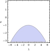
Figure 1. The region where $P\left(\frac{1}{\sqrt{5}},\lambda,\mu\right)>0$ is shaded.

5. The Dispersion Relation

The models derived here depend upon choices of six parameters, which have been denoted $\lambda,\lambda_{1},\mu,\mu_{1},\theta$ and $\rho$. The parameter $\theta$ has physical significance whereas the others are modeling parameters and in principle, can take any real value.

As will be seen in a moment, the linearized dispersion relation for the class of models derived here always matches that of the full water-wave problem through second order in the small parameter $\beta$. More precisely, if any of these models are linearized about the rest state, the resulting linear partial differential equation has a dispersion relation relating phase speed $c$ to wave number $k$. A brief calculation shows this to be

$$c_{model}(k)\,=\,1-\big{(}\gamma_{1}+\gamma_{2}\big{)}k^{2}+\big{(}\delta_{2}-\delta_{1}+\gamma_{1}^{2}+\gamma_{1}\gamma_{2}\big{)}k^{4}+\mathcal{F}k^{6}$$ (5.93)

where $k$ is the wave number and the coefficient $\mathcal{F}$ is

$$\mathcal{F}\,=\,\mathcal{F}(\theta,\lambda,\mu,\lambda_{1},\mu_{1},\rho)\,=\,-\gamma_{1}\delta_{2}-\gamma_{2}(-\delta_{1}+\gamma_{1}^{2})+2\gamma_{1}\delta_{1}-\gamma_{1}^{3}.$$ (5.94)

As $\gamma_{1}+\gamma_{2}=1/6$ holds independently of the choice of parameters, the second and third terms simplify, viz.

$$c_{model}(k)\,=\,1-\frac{1}{6}k^{2}+\left(\delta_{2}-\delta_{1}+\frac{1}{6}\gamma_{1}\right)k^{4}+\mathcal{F}k^{6},$$ (5.95)

where the coefficient $\mathcal{F}$ will be displayed presently. Making use of (4.87) leads to the final result

$$c_{model}(k)\,=\,1-\frac{1}{6}k^{2}+\left(\frac{19}{360}\right)k^{4}+\mathcal{F}k^{6},$$ (5.96)

regardless of the choice of the various parameters.

For the two-dimensional water wave problem displayed in (1.1), the linearized dispersion relationship is exactly

$$c_{Euler}(k)=\pm\sqrt{\frac{\tanh(k)}{k}}.$$ (5.97)

For waves moving to the right, the $+$–sign is appropriate. One recognizes that the Taylor expansion of the function of the right-hand side of (5.97) in the long wave regime (small wavenumber $k$) is

$$c_{Euler}(k)\,=\,1-\frac{1}{6}k^{2}+\frac{19}{360}k^{4}-\frac{55}{3024}k^{6}+O(k^{8}).$$

In consequence, all the models put forward here are seen to satisfy the full, linear dispersion relation through order $k^{4}$. Of course, if the derivation is done correctly, this has to be the case. If one rescales the variables so the long wavelength assumption is measured by $\beta$ as in the formalities of the derivation, then one sees that the error in the linear part of the approximation is at least of order $\beta^{3}$.

It is tempting to choose the parameters $\theta,\lambda,\mu,\lambda_{1},\mu_{1}$ and $\rho$ so that $\mathcal{F}$ matches the next order in the dispersion relation exactly, as was done at the lower order in [11]. Hence, if the auxiliary parameters are chosen so that

$$\mathcal{F}(\theta,\lambda,\mu,\lambda_{1},\mu_{1},\rho)=-\frac{55}{3024},$$ (5.98)

then the linear dispersion in the model would match that of the linear water wave problem up to and including order $\beta^{3}$. Such a choice could have a salutory effect on the detailed accuracy of the model, though it does not improve the overall formal level of approximation.

Of course, one needs that the criteria for local well posedness continue to hold in the light of this choice. A study of the formula (5.94) for $\mathcal{F}$ shows that

$$\begin{split}\mathcal{F}\,&=\,-\gamma_{1}\delta_{2}-\gamma_{2}\big{(}-\delta_{1}+\gamma_{1}^{2}\big{)}+2\gamma_{1}\delta_{1}-\gamma_{1}^{3}\\ &=\,-\gamma_{1}\delta_{2}+\delta_{1}\big{(}\gamma_{2}+2\gamma_{1}\big{)}-\gamma_{1}^{2}\big{(}\gamma_{1}+\gamma_{2}\big{)}\\ &=\,-\gamma_{1}\delta_{2}+\delta_{1}\left(\gamma_{1}+\frac{1}{6}\right)-\frac{1}{6}\gamma_{1}^{2}\\ &=\,\gamma_{1}\left(\delta_{1}-\delta_{2}-\frac{1}{6}\gamma_{1}\right)+\frac{1}{6}\delta_{1}\\ &=\,-\frac{19}{360}\gamma_{1}+\frac{1}{6}\delta_{1},\end{split}$$ (5.99)

where the facts that $\gamma_{1}+\gamma_{2}=1/6$ and the relation (4.86) have been used. It is interesting to know whether or not the relation (5.98), which implies the model dispersion relation agrees with the exact linear dispersion relation up to order $k^{6}$, is consistent with the conditions $\delta_{1}>0,\gamma_{1}>0$ and $\gamma=\frac{7}{48}$ implying global well posedness. The condition $\gamma=\frac{7}{48}$ requires that $\rho=b+d-\frac{1}{6}$ as in (4.84). This in turns implies that $\gamma_{1}=\frac{1}{12}>0$. That the parameters can be chosen so that (5.98) holds is clear upon consulting the formula (4.88) for $\delta_{1}$, which already presumes that $\rho=b+d-\frac{1}{6}$. For example, choose $\theta^{2}\in(\frac{1}{5},1)$, and fix $\lambda,\mu$ and $\mu_{1}$. Then $\delta_{1}$ is seen to have the form

$$\delta_{1}\,=\,M+N\lambda_{1}$$

where $N>0$. Clearly any value of $\delta_{1}$ can be achieved by a suitable choice of $\lambda_{1}$ and so any value of $\mathcal{F}$ can be achieved under the restriction $\rho=b+d-\frac{1}{6}$. However, notice that (5.99) and (5.98) yield

$$\delta_{1}\,=\,6\left(\frac{19}{360}\frac{1}{12}-\frac{55}{3024}\right)\,=\,-\frac{139}{1680}\,<\,0.$$ (5.100)

Hence, the requirement of Hamiltonian structure together with local well-posedness are not consistent with the model approximating the dispersion relation at the next order without considering $O(\alpha^{2},\beta^{2},\alpha\beta)$ terms in (2.23) and a new correction parameter like $\rho$.

6. Concluding Remarks

Derived here is a class of unidirectional models for long-crested water waves that are formally second-order correct. Basic analysis of the pure initial-value problem for our models has been developed. A local well-posedness theory in relatively weak spaces is established under conditions on the two parameters $\delta_{1}$ and $\gamma_{1}$ that appear in the model, and which depend upon the other parameters. Global well-posedness is only established in case the equation has a special, Hamiltonian structure. Conditions under which both aspects obtain are given.

A comment is deserved about the focus maintained throughout on unidirectional models. Boussinesq himself understood that his one-way model was simpler than the coupled pair of two-way models that he first derived. It was also simpler than a second-order in time, unidirectional model equation he had derived earlier. In both these instances, a modern perspective on this issue is that the undirectional model can be posed with half the auxiliary data needed to initiate the coupled system. However, unidirectionality places a severe limitation on the wave motion when it is posed as an initial-value problem. More precisely, a strict relationship between the initial wave profile and the velocity field is implied. On the other hand, it is known that for Boussinesq-type systems, if the initial disturbance is suitably localized and small, then on certain temporal scales, the disturbance will decompose into a left- and a right-going wave, each of which satisfy approximately a unidirectional equation (see [47], [18]). Finally, it is worth noting that even fairly steep beaches do not reflect all that much energy (see [41]). For very gently shelving beaches such as obtain in many nearshore zones, the reflection is negligible as regards its effect on shaping and erosive processes. Hence, unidirectional models seem to suffice in such circumstances.

Finallly, we remark that when choosing the depth parameter $\theta$, it is a good idea if it is taken well inside the interval $[0,1]$. While the horizontal velocity does not appear in the unidirectional model, a formal corollary of its derivation is a prediction of the horizontal velocity at the depth $1-\theta^{2}$. This is comprised of the formula (2.18) expressing the horizontal velocity in terms of the functions $A,B,C,D$ and $E$ together with the forms (2.17) determined for $A$ and $B$ and those for $C,D$ and $E$. It is hard to measure the horizontal velocity very close to the free surface, while in actual fact, there is no velocity on the bottom because of the viscous boundary layer. Typical velocity measurements in laboratory and field situations are made somewhere in the middle of the water column.

References

- [1]
- [2] A. A. Alazman, J. P. Albert, J. L. Bona, M. Chen and J. Wu; Comparisons between the BBM equation and a Boussinesq system, Advances in Differential Equations 11 (2006) 121–166.
- [3] D. M. Ambrose, J. L. Bona and D. P. Nicholls, Well-posedness of a model for water waves with viscosity, Discrete Contin. Dyn. Syst. Ser. B, 17 (2012) 1113–1137.
- [4] D. M. Ambrose, J. L. Bona and D. P. Nicholls, On ill-posedness of truncated series models for water waves, Proc. Royal Soc. London, Series A 470 (2014) 1–16.
- [5] D. M. Ambrose, J.L. Bona and T. Milgrom, Global solutions and ill-posedness for the Kaup system and related Boussinesq systems, Preprint.
- [6] C. J. Amick, J. L. Bona and M. E. Schonbek; Decay of solutions of some nonlinear wave equations, J. Diff. Eq. 81 (1989) 1–49.
- [7] T. B. Benjamin, J. L. Bona and J. J. Mahony; Model equations for long waves in nonlinear dispersive media, Philos. Trans. Royal Soc. London, Series A 272 (1972), 47–78.
- [8] B. Boczar-Karakiewicz, J. L. Bona, W. Romanczyk and E. Thornton; Seasonal and interseasonal variability of sand bars at Duck, NC, USA. Observations and model predictions, Preprint.
- [9] J. L. Bona; Nonlinear wave phenomena, Anais do Seminário Brasileiro de Análise 51 SBA, (Florianópolis), 2000.
- [10] J. L. Bona, H. Chen; Well-posedness for regularized nonlinear dispersive wave equations, Discrete Contin. Dyn. Syst. 23 (2009) 1253–1275.
- [11] J. L. Bona, M. Chen; A Boussinesq system for two-way propagation of nonlinear dispersive waves, Physica D 116 (1998) 191–224.
- [12] J. L. Bona, M. Chen and J.-C. Saut; Boussinesq equations and other systems for small-amplitude long waves in nonlinear dispersive media I. Derivation and linear theory, J. Nonlinear Sci. 12 (2002) 283–318.
- [13] J. L. Bona, M. Chen and J.-C. Saut; Boussinesq equations and other systems for small-amplitude long waves in nonlinear dispersive media II. The nonlinear theory, Nonlinearity 17 (2004) 925–952.
- [14] J. L. Bona, J. Cohen and G. Wang; Global well-posedness for a system of KdV-type equations with coupled quadratic nonlinearities, Nagoya Math. J. 215 (2014) 67–149.
- [15] J. L. Bona, M. Chen; Higher-order Boussinesq systems for two-way propagation of water waves, Proceedings of the Conferences on Nonlinear Evolutional Equations and Infinite-Dimensional Dynamical System held 12-16 June 1995, Shanghai, China (ed. Li Ta-Tsien) World Sci. Pub. Co.: Singapore (1997) 5–12.
- [16] J. L. Bona, M. Chen; Singular solutions of a Boussinesq system for water waves, J. Math. Study 49 (2016) 205–220.
- [17] J. L. Bona, T. Colin and C. Guillopé; Propagation of long-crested water waves, Discrete Contin. Dyn. Syst. 33 (2013) 599–628.
- [18] J. L. Bona, T. Colin and D. Lannes; Long Wave Approximations for Water Waves, Arch. Rational Mech. Anal. 178 (2005) 373–410.
- [19] J. L. Bona and H. Kalisch; Models for internal waves in deep water, Discrete Contin. Dyn. Syst. 6 (2000) 1–20.
- [20] J. L. Bona, W. G. Pritchard and L. R. Scott; An Evaluation of a Model Equation for Water Waves, Philos. Trans. Royal Soc. London Series A. 302 (1981) 457–510.
- [21] J. L. Bona, W. G. Pritchard and L. R. Scott; A comparison of solutions of two model equations for long waves, In Lectures in Applied Mathematics 20 (ed. N. Lebovitz) American Mathematical Society: Providence (1983) 235–267.
- [22] J. L. Bona and R. Smith; The initial-value problem for the Korteweg-de Vries equation, Philos. Trans. Royal Soc. London, Series A, 278 (1975) 555–601.
- [23] J. L. Bona and L. R. Scott; The Korteweg-de Vries equation in fractional order Sobolev spaces, Duke Math. J. 43 (1976) 87–99.
- [24] J. L. Bona and N. Tzvetkov; Sharp well-posedness results for the BBM equation, Discrete Contin. Dyn. Syst. 23 (2009) 1241–1252.
- [25] J. L. Bona and V. Varlmov; Wave generation by a moving boundary, In Nonlinear partial differential equations and related analysis, Contemporary Math. 371 (2005) (ed. G.-Q. Chen, G. Gasper and J. Jerome) American Math. Soc., Providence, RI, pp. 41–71.
- [26] J. Bourgain; Refinements of Strichartz inequality and applications to 2D-NLS with critical nonlinearity, IMRN 5 (1998) 253–283.
- [27] J. Boussinesq; Essai sur la theorie des eaux courantes, Memoires presentes par divers savants, l ’Acad. des Sci. Inst. Nat. France, XXIII (1877) 1–-680.
- [28] H. Chen; Well-posedness for a higher-order, nonlinear, dispersive equation on a quarter plane, submitted.
- [29] A. Constantin, D. Lannes; The hydrodynamical relevance of the Camassa-Holm and Degasperis-Processi equations, Arch. Rational Mech. Anal. 192 (2009) 165–186.
- [30] V. Duchêne; Decoupled and unidirectional asymptotic models for the propagation of internal waves, Math. Models Methods Appl. Sci. 24 (2014) 1–65.
- [31] H. R. Dullin, G. A. Gottwald and D. D. Holm; Camassa-Holm, Korteweg-de Vries-5, and other asymptotically equivalent models for shallow water waves. Fluid Dyn. Res. 33 (2003) 73–95.
- [32] G. Fonseca, F. Linares, G. Ponce; Global well-posedness for the modified Korteweg-de Vries equation, Communications in Partial Differential Equations 24 (1999) 683–70.
- [33] G. Fonseca, F. Linares, G. Ponce; Global existence for the critical generalized KdV equation, Proc. AMS 131 (2002) 1847–1855.
- [34] J. Hadamard; Sur les problèmes aux dérivées partielles et leur signification physique, Princeton University Bulletin 13 (1902) 49–52.
- [35] J. L. Hammack; A note on tsunamis, their generation and propagation in an ocean of uniform depth, J. Fluid Mech. 60 (1973) 769–799.
- [36] J. L. Hammack and H. Segur; The Korteweg-de Vries equation and water waves. Part 2. Comparison with experiments, J. Fluid Mech. 65 289–314
- [37] R. S. Johnson; 2002.Camassa–-Holm, Korteweg-–de Vries and related models for water waves, J. Fluid Mech. 455 (2002) 63–-82.
- [38] D. Lannes; The water waves problem: mathematical analysis and asymptotics, Math. Surveys and Monographs 188 (2013) (American Math. Soc.: Providence).
- [39] D. Lannes and J.-C. Saut; Weakly transverse Boussinesq systems and the Kadomtsev-Petviashvili approximation, Nonlinearity 19 (2006) 2853–2875.
- [40] F. Linares and G. Ponce; Introduction to Nonlinear Dispersive Equations, ed., Springer, Universitext, 2015.
- [41] J. J. Mahony and W. G. Pritchard; Wave reflexion from beaches, J. Fluid Mech. 101 (1980) 809–832.
- [42] T. R. Marchant and N. F. Smyth; 1990. The extended Korteweg–de Vries equation and the resonant flow over topography. J. Fluid Mech. 221 (1990) 263–288.
- [43] P. J. Olver; Hamiltonian and non-Hamiltonian models for water waves, Trends and applications of pure mathematics to mechanics (Palaiseau, 1983), Lecture Notes in Phys. 195 Springer: Berlin (1984) 273–290.
- [44] P. J. Olver; Hamiltonian perturbation theory and water waves, Contemp. Math. 28 (1984) 231–249.
- [45] D. H. Peregrine; Calculations of the development of an undular bore, J. Fluid Mech. 25 (1966) 321–330.
- [46] J.-C. Saut; Lectures on Asymptotic Models for Internal Waves, Lectures on the Analysis of Nonlinear Partial Differential Equations Vol. 2 MLM2, 147–201.
- [47] G. Schneider and C. E. Wayne. The long-wave limit for the water wave problem. I. The case of zero surface tension. Comm. Pure Appl. Math 53 (2000) 1475–1535.
- [48] M. E. Schonbek; Existence of solutions for the Boussinesq system of equations, J. Diff. Eq. 42 (1981) 325–352.
- [49] G. B. Whitham; Linear and Nonlinear Waves (1999) Wiley: New York.
- [50] V. Zakharov; Stability of periodic waves of finite amplitude on the surface of a deep fluid, J. Appl. Mech. and Tech. Phys., 9 (1968) 190–194.