Boolean Matrix Factorization and Noisy Completion via Message Passing

Abstract

Boolean matrix factorization and Boolean matrix completion from noisy observations are desirable unsupervised data-analysis methods due to their interpretability, but hard to perform due to their NP-hardness. We treat these problems as maximum a posteriori inference problems in a graphical model and present a message passing approach that scales linearly with the number of observations and factors. Our empirical study demonstrates that message passing is able to recover low-rank Boolean matrices, in the boundaries of theoretically possible recovery and compares favorably with state-of-the-art in real-world applications, such collaborative filtering with large-scale Boolean data.

A body of problems in machine learning, communication theory and combinatorial optimization involve the product form ${{{Z}}}={{{X}}}\odot{{{Y}}}$ where $\odot$ operation corresponds to a type of matrix multiplication and

$${{{Z}}}=\{{{Z}}_{{m},{n}}\}^{{M}\times{N}},{{{X}}}=\{{{X}}_{{m},{k}}\}^{{M}\times{K}},{{{Y}}}=\{{{Y}}_{{k},{n}}\}^{{K}\times{N}}.$$

Here, often one or two components out of three are (partially) known and the task is to recover the unknown component(s).

A subset of these problems, which are most closely related to Boolean matrix factorization and matrix completion, can be expressed over the Boolean domain – i.e., ${{Z}}_{{m},{n}},\ {{X}}_{{m},{k}},\ {{Y}}_{{k},{n}}\ \in\ \{\mathrm{false},\,\mathrm{true}\}\cong\{0,\,1\}$. The two most common Boolean matrix products used in such applications are

$${{{Z}}}={{{X}}}\bullet{{{Y}}}\Rightarrow{{Z}}_{{m},{n}}=\bigvee_{{k}=1}^{{K}}{{X}}_{{m},{k}}\wedge{{Y}}_{{k},{n}}$$ (1a)

$${{{Z}}}={{{X}}}\ast{{{Y}}}\Rightarrow{{Z}}_{{m},{n}}\equiv\big{(}\sum_{{k}=1}^{{K}}{{X}}_{{m},{k}}\wedge{{Y}}_{{k},{n}}\big{)}\mod 2$$ (1b)

where we refer to Equation 1a simply as Boolean product and we distinguish Equation 1b as exclusive-OR (XOR) Boolean product. One may think of Boolean product as ordinary matrix product where the values that are larger than zero in the product matrix are set to one. Alternatively, in XOR product, the odd (even) numbers are identically set to one (zero) in the product matrix.

This model can represent Low Density Parity Check (LDPC) coding using the XOR product, with $N=1$. In LDPC, the objective is to transmit the data vector ${{{Y}}}\in\{0,1\}^{{K}}$ though a noisy channel. For this, it is encoded by Equation 1b, where ${{{X}}}\in\{0,1\}^{{m}\times{k}}$ is the parity check matrix and vector ${{{Z}}}\{0,1\}^{{M}}$ is then sent though the channel with a noise model ${{p}^{{{{O}}}}}({{{O}}}\mid{{{Z}}})$, producing observation ${{{O}}}$. Message passing decoding has been able to transmit ${{{Z}}}$ and recover ${{{Y}}}$ from ${{{O}}}$ at rates close to the theoretical capacity of the communication channel (Gallager, 1962).

LDPC codes are in turn closely related to the compressed sensing (Donoho, 2006) – so much so that successful binary LDPC codes (i.e., matrix ${{{X}}}$) have been reused for compressed sensing (Dimakis et al., 2012). In this setting, the column-vector ${{{Y}}}$ is known to be $\ell$-sparse (i.e., $\ell$ non-zero values) which makes it possible to use approximate message passing (Donoho et al., 2009) to recover ${{{Y}}}$ using few noisy measurements ${{{O}}}$ – that is ${M}\ll{K}$ and similar to LDPC codes, the measurement matrix ${{{X}}}$ is known. When the underlying domain and algebra is Boolean (i.e., Equation 1a), the compressed sensing problem reduces to the problem of (noisy) group testing (Du and Hwang, 1993) where message passing has been successfully applied in this setting as well (Atia and Saligrama, 2012; Sejdinovic and Johnson, 2010).

These problems over Boolean domain are special instances of the problem of Boolean factor analysis in which ${{{Z}}}$ is given, but not ${{{X}}}$ nor ${{{Y}}}$. Here, inspired by the success of message passing techniques in closely related problems over “real” domain, we derive message passing solutions to a novel graphical model for “Boolean” factorization and matrix completion, and show that simple application of Belief Propagation (BP; Pearl, 1982) to this graphical model favorably compares with the state-of-the-art in both Boolean factorization and completion.

In the following, we briefly introduce the Boolean factorization and completion problems in Section -A and Section I reviews the related work. Section II formulates both of these problems in a Bayesian framework using a graphical model. The ensuing message passing solution is introduced in Section III. Experimental study of Section IV demonstrates that message passing is an efficient and effective method for performing Boolean matrix factorization and noisy completion.

-A Boolean Factor Analysis

The umbrella term “factor analysis” refers to the unsupervised methodology of expressing a set of observations in terms of unobserved factors (McDonald, 2014). In contrast to LDPC and compressed sensing, in factor analysis, only (a partial and/or distorted version of) the matrix ${{{Z}}}$ is observed, and our task is then to find ${{{X}}}$ and ${{{Y}}}$ whose product is close to ${{{Z}}}$. When the matrix ${{{Z}}}$ is partially observed, a natural approach to Boolean matrix completion is to find sparse and/or low-rank Boolean factors that would lead us to missing elements of ${{{Z}}}$. In the following we focus on the Boolean product of Equation 1a, noting that message passing derivation for factorization and completion using the XOR product of Equation 1b is similar.

The “Boolean” factor analysis – including factorization and completion – has a particularly appealing form. This is because the Boolean matrix ${{{Z}}}$ is simply written as disjunction of Boolean matrices of rank one – that is ${{{Z}}}=\bigvee_{{k}=1}^{{K}}{{{X}}}_{:,k}\bullet{{{Y}}}_{k,:}$, where ${{{X}}}_{:,k}$ and ${{{Y}}}_{k,:}$ are column vector and row vectors of ${{{X}}}$ and ${{{Y}}}$ respectively.

-A1 Combinatorial Representation

The combinatorial representation of Boolean factorization is the biclique cover problem in a bipartite graph $\mathcal{G}=(\mathcal{A}\cup\mathcal{B},\mathcal{E})$. Here a bipartite graph has two disjoint node sets $\mathcal{A}$ (s.t. $|\mathcal{A}|={M}$) and $\mathcal{B}$ (s.t. $|\mathcal{B}|={N}$) where the only edges are between these two sets – i.e., $\mathcal{E}\subseteq\{(a,b)\mid a\in\mathcal{A},\;b\in\mathcal{B}\}$. In our notation ${{{Z}}}\in\{0,1\}^{M\times N}$ represents the incident matrix of $\mathcal{G}$ and the objective of factorization is to cover (only) the edges using ${K}$ bicliques (i.e., complete bipartite sub-graphs of $\mathcal{G}$). Here the ${k}^{th}$ biclique is identified with a subset of $\mathcal{A}$, corresponding to ${{{X}}}_{:,{k}}$, the ${k}^{th}$ column of ${{{X}}}$, and a subset of $\mathcal{B}$, ${{{Y}}}_{k,:}$, corresponding to the ${k}^{th}$ row of ${{{Y}}}$ the Boolean product of which is a Boolean matrix of rank $1$. The disjunction of these rank 1 matrices is therefore a biclique covering of the incident matrix $Z$.

I Applications and Related Work

Many applications of Boolean factorization are inspired by its formulation as tiling problem (Stockmeyer, 1975). Examples include mining of Boolean databases (Geerts et al., 2004) to role mining (Vaidya et al., 2007; Lu et al., 2008) to bi-clustering of gene expression data (Zhang et al., 2010). Several of these applications are accompanied by a method for approximating the Boolean factorization problem.

The most notable of these is the “binary” factorization of Zhang et al. (2010) that uses an alternating optimization method to repeatedly solve a penalized non-negative matrix factorization problem over real-domain, where the penalty parameters try to enforce the desired binary form. Note that a binary matrix factorization is generally a more constrained problem than Boolean factorization and therefore it also provides a valid Boolean factorization.

Among the heuristics (e.g.,  Keprt and Snásel, 2004; Belohlavek et al., 2007) that directly apply to Boolean factorization, the best known is the Asso algorithm of Miettinen et al. (2006). Since Asso is incrmental in ${K}$, it can efficiently use the Minimum Description Length principle to select the best rank $K$ by incrementing its value (Miettinen and Vreeken, 2011).

An important application of Boolean matrix completion is in collaborative filtering with Boolean (e.g., like/dislike) data, where the large-scale and sparsely observed Boolean matrices in modern applications demands a scalable and accurate Boolean matrix completion method.

One of the most scalable methods for this problem is obtained by modeling the problem as a Generalized Low Rank Model (GLRM; Udell et al., 2014), that uses proximal gradient for optimization. Using logistic or hinge loss can enforce binary values for missing entries. Using the hinge loss, GLRM seeks

$$\arg\min_{{{{X}}},{{{Y}}}}\sum_{({m},{n})\in\Omega}\big{(}1-(\sum_{{k}}{{X}}_{{m},{k}}{{Y}}_{{k},{n}})(2{{O}}_{{m},{n}}-1)\big{)}_{+}$$

, where $(2{{O}}_{{m},{n}}-1)$ changes the domain of observations to $\{-1,+1\}$ and $\Omega$ is index-set of observed elements.

In the 1-Bit matrix completion of Davenport et al. (2014), the single bit observation ${{O}}_{{m},{n}}$ from a hidden real-valued matrix ${{{Q}}}$ is obtained by sampling from a distribution with the cumulative distribution function $f({{Q}}_{{m},{n}})$ – e.g., ${\mathsf{f}}({{Q}}_{{m},{n}})=(1+\exp(-{{Q}}_{{m},{n}}))^{-1}$. For application to Boolean completion, our desired Boolean matrix is ${{{Z}}}=\mathbb{I}(f({{{Q}}}){\geq}.5)$. 1-Bit completion then minimizes the likelihood of observed entries, while constraining the nuclear norm of ${{{Q}}}$

$$\arg\min_{{{{Q}}}}\; \sum_{({m},{n})\in\Omega}\bigg{(}{{O}}_{{m},{n}}\log(f({{Q}}_{{m},{n}}))+$$ (2)

$${{O}}_{{m},{n}}\log(1-f({{Q}}_{{m},{n}}))\bigg{)}\quad s.t.\;\|{{{Q}}}\|_{*}\leq\beta\sqrt{{K}{M}{N}},$$

where $\beta>0$ is a hyper-parameter.

In another recent work, Maurus and Plant (2014) introduce a method of ternary matrix factorization that can handle missing data in Boolean factorization through ternary logic. In this model, the ternary matrix ${{{Z}}}$ is factorized to ternary product of a binary matrix ${{{X}}}$ and a ternary basis matrix ${{{Y}}}$.

II Bayesian Formulation

Expressing factorization and completion problems as a MAP inference problem is not new (e.g.,  Mnih and Salakhutdinov, 2007), neither is using message passing as an inference technique for these problems (Krzakala et al., 2013; Parker et al., 2013; Kabashima et al., 2014). However, message passing has not been previously used to solve the “Boolean” factorization/completion problem.

To formalize approximate decompositions for Boolean data, we use a communication channel, where we assume that the product matrix ${{{Z}}}$ is communicated through a noisy binary erasure channel (Cover and Thomas, 2012) to produce the observation ${{{O}}}\in\{0,1,\mathrm{null}\}^{{M}\times{N}}$ where ${{O}}_{{m},{n}}=\mathrm{null}$, means this entry was erased in the channel. This allows us to model matrix completion using the same formalism that we use for low-rank factorization.

For simplicity, we assume that each element of ${{{Z}}}$ is independently transmitted (that is erased, flipped or remains intact) through the channel, meaning the following conditional probability completely defines the noise model:

$${{p}^{{{{O}}}}}({{{O}}}\mid{{{Z}}})=\prod_{{m},{n}}{{p}^{{{{O}}}}}_{{m},{n}}({{O}}_{{m},{n}}\mid{{Z}}_{{m},{n}})$$ (3)

Note that each of these conditional probabilities can be represented using six values – one value per each pair of ${{O}}_{{m},{n}}\in\{0,1,\mathrm{null}\}$ and ${{Z}}_{{m},{n}}\in\{0,1\}$. This setting allows the probability of erasure to depend on the value of $m$, $n$ and ${{Z}}_{{m},{n}}$.

The objective is to recover ${{{X}}}$ and ${{{Y}}}$ from ${{{O}}}$. However, due to its degeneracy, recovering ${{{X}}}$ and ${{{Y}}}$ is only up to a ${K}\times{K}$ permutation matrix ${{{U}}}$ – that is ${{{X}}}\bullet{{{Y}}}=({{{X}}}\bullet{{{U}}})\bullet({{{U}}}^{T}\bullet{{{Y}}})$. A Bayesian approach can resolve this ambiguity by defining non-symmetric priors

$${{p}^{{{{X}}}}}({{{X}}})=\prod_{{m},{k}}{{p}^{{{{X}}}}}_{{m},{k}}({{X}}_{{m},{k}})$$ (4a)

$${{p}^{{{{Y}}}}}({{{Y}}})=\prod_{{k},{n}}{{p}^{{{{Y}}}}}_{{k},{n}}({{Y}}_{{k},{n}})$$ (4b)

where we require the a separable product form for this prior. Using strong priors can enforce sparsity of ${{{X}}}$ and/or ${{{Y}}}$, leading to well-defined factorization and completion problems where $K>M,N$.

Now, we can express the problem of recovering ${{{X}}}$ and ${{{Y}}}$ as a maximum a posteriori (MAP) inference problem
$\arg\max_{{{{X}}},{{{Y}}}}\;{p}({{{X}}},{{{Y}}}\mid{{{O}}})$, where the posterior is

$${p}({{{X}}},{{{Y}}}\mid{{{O}}})\;\propto\;{{p}^{{{{X}}}}}({{{X}}})\;{{p}^{{{{Y}}}}}({{{Y}}})\;{{p}^{{{{O}}}}}({{{O}}}\mid{{{X}}}\bullet{{{Y}}})$$ (5)

Finding the maximizing assignment for Equation 5 is ${NP}$-hard (Stockmeyer, 1975). Here we introduce a graphical model to represent the posterior and use a simplified form of BP to approximate the MAP assignment.

An alternative to finding the MAP assignment is that of finding the marginal-MAP – i.e.,

$$\arg\max_{{{{X}}}_{{m},{k}}}{p}({{X}}_{{m},{k}}\mid{{{O}}})=\arg\max_{{{{X}}}_{{m},{n}}}\sum_{{{{X}}}\backslash{{X}}_{i},{{{Y}}}}{p}({{{X}}},{{{Y}}}\mid{{{O}}}).$$

While the MAP assignment is the optimal “joint” assignment to ${{{X}}}$ and ${{{Y}}}$, finding the marginal-MAP corresponds to optimally estimating individual assignments for each variable, while the other variable assignments are marginalized. We also provide the message passing solution to this alternative in Appendix B.

II-A The Factor-Graph

Figure 1 shows the factor-graph (Kschischang et al., 2001) representation of the posterior Equation 5. Here, variables are circles and factors are squares. The factor-graph is a bipartite graph, connecting each factor/function to its relevant variables. This factor-graph has one variable ${{X}}_{{m},{k}}\in\{0,1\}$ for each element of ${{{X}}}$, and a variable ${{Y}}_{{k},{n}}\in\{0,1\}$ for each element of ${{{Y}}}$. In addition to these ${K}\times({M}+{N})$ variables, we have introduced ${K}\times{M}\times{N}$ auxiliary variables ${{W}}_{{m},{n},{k}}\in\{0,1\}$. For Boolean matrix completion the number of auxiliary variables is ${K}|\Omega|$, where $\Omega=\{({m},{n})|{{O}}_{{m},{n}}\neq\mathrm{null}\}$ is the set of observed elements (see Section III-A).

We use plate notation (often used with directed models) in representing this factor-graph. Figure 1 has three plates for $1\leq{m}\leq{M}$, $1\leq{n}\leq{N}$ and $1\leq{k}\leq{K}$ (large transparent boxes in Figure 1). In plate notation, all variables and factors on a plate are replicated. For example, variables on the $m$-plate are replicated for $1\leq{m}\leq{M}$. Variables and factors located on more than one plate are replicated for all combinations of their plates. For example, since variable ${{X}}$ is in common between ${m}$-plate and ${k}$-plate, it refers to ${M}\times{K}$ binary variables – i.e., ${{X}}_{{m},{k}}\;\forall{m},{k}$.

II-A1 Variables and Factors

The auxiliary variable ${{W}}_{{m},{n},{k}}$ represents the Boolean product of ${{X}}_{m,{k}}$ and ${{Y}}_{{k},{n}}$ – i.e., ${{W}}_{{m},{n},{k}}={{X}}_{m,{k}}\wedge{{Y}}_{{k},{n}}$. This is achieved through ${M}\times{N}\times{K}$ hard constraint factors

$${\mathsf{f}}_{{m},{n},{k}}({{X}}_{{m},{k}},{{Y}}_{{k},{n}},{{W}}_{{m},{n},{k}})\;=\;\mathbb{I}({{W}}_{{m},{n},{k}}={{X}}_{m,{k}}\wedge{{Y}}_{{k},{n}})$$

where $\mathbb{I}(.)$ is the identity function on the inference semiring (see Ravanbakhsh and Greiner, 2014). For the max-sum inference $\mathbb{I}_{\text{max-sum}}(\mathrm{true})=0$ and $\mathbb{I}_{\text{max-sum}}(\mathrm{false})=-\infty$.

Local factors ${\mathsf{h}}_{{m},{k}}({{X}}_{{m},{k}})\;=\;\log({{p}^{{{{X}}}}}({{X}}_{{m},{k}}))$ and ${\mathsf{h}}_{{k},{n}}({{Y}}_{{k},{n}})\;=\;\log({{p}^{{{{Y}}}}}({{Y}}_{{k},{n}}))$ represent the logarithm of priors over ${{{X}}}$ and ${{{Y}}}$ in Equation 5.

Finally, the noise model in Equation 5 is represented by ${M}\times{N}$ factors over auxiliary variables

$${\mathsf{g}}_{{m},{n}}(\{{{W}}_{{m},{n},{k}}\}_{1\leq{k}\leq{K}})=\log\bigg{(}{{p}^{{{{O}}}}}_{{m},{n}}({{O}}_{{m},{n}}\mid\bigvee_{{k}}{{W}}_{{m},{n},{k}})\bigg{)}.$$

Although our introduction of auxiliary variables is essential in building our model, the factors of this type have been used in the past. In particular, factor ${\mathsf{g}}$ is generalized by a high-order family of factors with tractable inference, known as cardinality-based potentials (Gupta et al., 2007). This factor is also closely related to noisy-or models (Pearl, 2014; Middleton et al., 1991); where MCMC (Wood et al., 2012) and variational inference (Šingliar and Hauskrecht, 2006) has been used to solve more sophisticated probabilistic models of this nature.

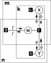
Figure 1: The factor-graph and the message exchange between variables and factors.

The combination of the factors of type ${\mathsf{g}}$ and ${\mathsf{f}}$, represent the term ${p}({{O}}_{{m},{n}}\mid\bigvee_{{k}=1}^{{K}}{{X}}_{{m},{k}}\wedge{{Y}}_{{k},{n}})$ in Equation 5 and the local factors ${\mathsf{h}}$, represent the logarithm of the priors. It is easy to see that the sum of all the factors above, evaluates to the logarithm of the posterior

$$\log({p}({{{X}}},{{{Y}}}\mid{{{O}}}) =\sum_{{{m},{k}}}{\mathsf{h}}_{{m},{k}}({{X}}_{{m},{k}})+\sum_{{k},{n}}{\mathsf{h}}_{{k},{n}}({{X}}_{{k},{n}})$$

$$+\sum_{{m},{n}}{\mathsf{g}}_{{m},{n}}(\{{{X}}_{m,{k}}\wedge{{Y}}_{{k},{n}}\}_{1\leq{k}\leq{K}})$$

if ${{W}}_{{m},{n},{k}}={{X}}_{m,{k}}\wedge{{Y}}_{{k},{n}}\,\forall{m},{n},{k}$ and $-\infty$ otherwise. Therefore, maximizing the sum of these factors is equivalent to MAP inference for Equation 5.

III Message Update

Input: 1) observed matrix ${{{O}}}\in\{0,1\}^{{M}\times{N}}\;\forall m,n$;

2) ${K}\in\mathbb{N}$;

3) priors ${{p}^{{{{X}}}}}_{{m},{k}},{{p}^{{{{Y}}}}}_{{n},{k}}\;\forall m,n,k$;

4) noise model ${{p}^{{{{O}}}}}_{{m},{n}}\;\forall m,n,k$

Output: ${{{X}}}\in\{0,1\}^{{M}\times{K}}$ and ${{{Y}}}\in\{0,1\}^{{K}\times{N}}$.

$t:=0$

init $\Phi_{{m},{n},{k}}^{(\mathrm{t})},\Psi_{{m},{n},{k}}^{(\mathrm{t})},\hat{\Phi}_{{m},{n},{k}}^{(\mathrm{t})},\hat{\Psi}_{{m},{n},{k}}^{(\mathrm{t})},\hat{\Gamma}_{{m},{n},{k}}^{(\mathrm{t})}$ and $\Gamma_{{m},{n},{k}}^{(\mathrm{t})}\;\;\;\;\forall{m},{n},{k}$

while $t<T_{\max}$ and not converged for all $m,n,k$ do

  

$$\Phi_{{m},{n},{k}}^{(\mathrm{t+1})}:=\big{(}\Gamma_{{m},{n},{k}}^{(\mathrm{t})}+\hat{\Psi}_{{m},{n},{k}}^{(\mathrm{t})}\big{)}_{+}\,-\,\big{(}\hat{\Psi}_{{m},{n},{k}}^{(\mathrm{t})}\big{)}_{+}$$ (6a)

$$\Psi_{{m},{n},{k}}^{(\mathrm{t+1})}:=\big{(}\Gamma_{{m},{n},{k}}^{(\mathrm{t})}+\hat{\Phi}_{{m},{n},{k}}^{(\mathrm{t})}\big{)}_{+}\,-\,\big{(}\hat{\Phi}_{{m},{n},{k}}^{(\mathrm{t})}\big{)}_{+}$$ (6b)

$$\hat{\Phi}_{{m},{n},{k}}^{(\mathrm{t+1})}:=\log\bigg{(}\frac{{{p}^{{{{X}}}}}_{{m},{k}}(1)}{{{p}^{{{{X}}}}}_{{m},{k}}(0)}\bigg{)}+\sum_{{n}^{\prime}\neq{n}}\;\Phi_{{m},{n}^{\prime},{k}}^{(\mathrm{t})}$$ (6c)

$$\hat{\Psi}_{{m},{n},{k}}^{(\mathrm{t+1})}:=\log\bigg{(}\frac{{{p}^{{{{Y}}}}}_{{n},{k}}(1)}{{{p}^{{{{Y}}}}}_{{n},{k}}(0)}\bigg{)}+\sum_{{m}^{\prime}\neq{m}}\;\Psi_{{m}^{\prime},{n},{k}}^{(\mathrm{t})}$$ (6d)

$$\hat{\Gamma}_{{m},{n},{k}}^{(\mathrm{t+1})}:=\min\bigg{\{}\hat{\Phi}_{{m},{n},{k}}^{(\mathrm{t})}+\hat{\Psi}_{{m},{n},{k}}^{(\mathrm{t})},$$

$$\quad\quad\quad\quad\quad\quad\quad\hat{\Phi}_{{m},{n},{k}}^{(\mathrm{t})},\hat{\Psi}_{{m},{n},{k}}^{(\mathrm{t})}\bigg{\}}$$ (6e)

$$\Gamma_{{m},{n},{k}}^{(\mathrm{t+1})}:=\min\bigg{\{}\big{(}-\max_{{k}^{\prime}\neq{k}}\hat{\Gamma}_{{m},{n},{k}^{\prime}}^{(\mathrm{t})}\big{)}_{+},$$

$$\sum_{{k}^{\prime}\neq{k}}\big{(}\hat{\Gamma}_{{m},{n},{k}^{\prime}}^{(\mathrm{t})}\big{)}_{+}+\log\bigg{(}\frac{{{p}^{{{{O}}}}}_{{m},{n}}({{O}}_{{m},{n}}\mid 1)}{{{p}^{{{{O}}}}}_{{m},{n}}({{O}}_{{m},{n}}\mid 0)}\bigg{)}\bigg{\}}$$ (6f)

   end while

  

  calculate log-ratio of the posterior marginals

  

$$\Xi_{{m},{k}}:=\log\bigg{(}\frac{{{p}^{{{{X}}}}}_{{m},{k}}(1)}{{{p}^{{{{X}}}}}_{{m},{k}}(0)}\bigg{)}+\sum_{{n}}\Phi_{{m},{n},{k}}^{(\mathrm{t})}$$ (7a)

$$\Upsilon_{{k},{n}}:=\log\bigg{(}\frac{{{p}^{{{{Y}}}}}_{{k},{n}}(1)}{{{p}^{{{{Y}}}}}_{{k},{n}}(0)}\bigg{)}+\sum_{{m}}\Psi_{{m},{n},{k}}^{(\mathrm{t})}$$ (7b)

  calculate ${{{X}}}$ and ${{{Y}}}$

  

$${{X}}_{{m},{k}}:=\begin{cases}1,&\text{if}\;\Xi_{{m},{k}}>0\\ 0,&\text{otherwise}\end{cases}$$ (8a)

$${{Y}}_{{k},{n}}:=\begin{cases}1,&\text{if}\;\Upsilon_{{k},{n}}>0\\ 0,&\text{otherwise}\end{cases}$$ (8b)

return ${{{X}}}$,${{{Y}}}$

Algorithm 1 message passing for Boolean matrix factorization/completion

Max-sum Belief Propagation (BP) is a message passing procedure for approximating the MAP assignment in a graphical model. In factor-graphs without loops, max-sum BP is simply an exact dynamic programming approach that leverages the distributive law. In loopy factor-graphs the approximations of this message passing procedure is justified by the fact that it represents the zero temperature limit to the sum-product BP, which is in turn a fixed point iteration procedure whose fixed points are the local optima of the Bethe approximation to the free energy (Yedidia et al., 2000); see also (Weiss et al., 2012). For general factor-graphs, it is known that the approximate MAP solution obtained using max-sum BP is optimal within its “neighborhood” (Weiss and Freeman, 2001).

We apply max-sum BP to approximate the MAP assignment of the factor-graph of Figure 1. This factor-graph is very densely connected and therefore, one expects BP to oscillate or fail to find a good solution. However, we report in Section IV that BP performs surprisingly well. This can be attributed to the week influence of majority of the factors, often resulting in close-to-uniform messages. Near-optimal behavior of max-sum BP in dense factor-graph is not without precedence (e.g.,  Frey and Dueck, 2007; Decelle et al., 2011; Ravanbakhsh et al., 2014).

The message passing for MAP inference of Equation 5 involves message exchange between all variables and their neighboring factors in both directions. Here, each message is a Bernoulli distribution. For example $\mathfrak{m}_{{{X}}_{{m},{k}}\to{\mathsf{f}}_{{m},{n},{k}}}({{X}}_{{m},{n}}):\{0,1\}\to\Re^{2}$ is the message from variable node ${{X}}_{{m},{n}}$ to the factor node ${\mathsf{f}}_{{m},{n},{k}}$. For binary variables, it is convenient to work with the log-ratio of messages – e.g., we use $\hat{\Phi}_{{m},{n},{k}}=\log\big{(}\frac{\mathfrak{m}_{{{X}}_{{m},{k}}\to{\mathsf{f}}_{{m},{n},{k}}}(1)}{\mathfrak{m}_{{{X}}_{{m},{k}}\to{\mathsf{f}}_{{m},{n},{k}}}(0)}\big{)}$ and the log-ratio of the message is opposite direction is denoted by $\hat{\Phi}$. Messages $\Psi$, $\hat{\Psi}$, $\hat{\Gamma}$ and $\Gamma$ in Figure 1 are defined similarly. For a review of max-sum BP and the detailed derivation of the simplified BP updates for this factor-graph, see Appendix A. In particular, a naive application of BP to obtain messages $\Gamma_{{m},{n}}$ from the likelihood factors ${\mathsf{g}}_{{m},{n}}(\{{{W}}_{{m},{n},{k}}\}_{1\leq{k}\leq{K}})\;\forall{m},{n}$ to the auxiliary variables ${{W}}_{{m},{n},{k}}$ has a $\mathcal{O}(2^{{K}})$ cost. In Appendix A, we show how this can be reduced to $\mathcal{O}({K})$. Algorithm 1 summarizes the simplified message passing algorithm.

At the beginning of the Algorithm, $t=0$, messages are initialized with some random value – e.g., using $\log(U)-\log(1-U)$ where $U\sim\mathrm{Uniform(0,1)}$. Using the short notation $\big{(}a\big{)}_{+}\;=\;\max\{0,a\}$, at time $t+1$, the messages are updated using 1) the message values at the previous time step $t$; 2) the prior; 3) the noise model and observation ${{{O}}}$. The message updates of Equation 6 are repeated until convergence or a maximum number of iterations $T_{\max}$ is reached. We decide the convergence based on the maximum absolute change in one of the message types e.g., $\max_{{m},{n},{k}}|\Phi_{{m},{n},{k}}^{(\mathrm{t+1})}-\Phi_{{m},{n},{k}}^{(\mathrm{t})}|\overset{?}{\leq}\epsilon$.

Once the message update converges, at iteration $T$, we can use the values for $\Phi_{{m},{n},{k}}^{(\mathrm{T})}$ and $\Psi_{{m},{n},{k}}^{(\mathrm{T})}$ to recover the log-ratio of the marginals ${p}({{X}}_{{m},{k}})$ and ${p}({{Y}}_{{n},{k}})$. These log-ratios are denoted by $\Xi_{{m},{k}}$ and $\Upsilon_{{k},{n}}$ in Equation 7. A positive log-ratio $\Xi_{{m},{k}}>0$ means ${p}({{X}}_{{m},{k}}=1)>{p}({{X}}_{{m},{k}}=0)$ and the posterior favors ${{X}}_{{m},{k}}=1$. In this way the marginals are used to obtain an approximate MAP assignment to both ${{{X}}}$ and ${{{Y}}}$.

For better convergence, we also use damping in practice. For this, one type of messages is updated to a linear combination of messages at time $t$ and $t+1$ using a damping parameter ${\lambda}\in(0,1]$. Choosing $\hat{\Phi}$ and $\hat{\Psi}$ for this purpose, the updates of Equations 6c and 6d become

$$\hat{\Phi}_{{m},{n},{k}}^{(\mathrm{t+1})} :=(1-{\lambda})\hat{\Phi}_{{m},{n},{k}}^{(\mathrm{t})}+$$ (9)

$${\lambda}\bigg{(}\log\bigg{(}\frac{{{p}^{{{{X}}}}}_{{m},{k}}(1)}{{{p}^{{{{X}}}}}_{{m},{k}}(0)}\bigg{)}+\sum_{{n}^{\prime}\neq{n}}\Phi_{{m},{n}^{\prime},{k}}^{(\mathrm{t})}\bigg{)},$$

$$\hat{\Psi}_{{m},{n},{k}}^{(\mathrm{t+1})} :=(1-{\lambda})\hat{\Psi}_{{m},{n},{k}}^{(\mathrm{t})}+$$

$${\lambda}\bigg{(}\log\bigg{(}\frac{{{p}^{{{{Y}}}}}_{{n},{k}}(1)}{{{p}^{{{{Y}}}}}_{{n},{k}}(0)}\bigg{)}+\sum_{{m}^{\prime}\neq{m}}\Psi_{{m}^{\prime},{n},{k}}^{(\mathrm{t})}\bigg{)}.$$

III-A Further Simplifications

Partial knowledge. If any of the priors, ${p}({{X}}_{{m},{k}})$ and ${p}({{Y}}_{{n},{k}})$, are zero or one, it means that ${{{X}}}$ and ${{{Y}}}$ are partially known. The message updates of Equations 6c and 6d will assume $\pm\infty$ values, to reflect these hard constrains. In contrast, for uniform priors, the log-ratio terms disappear.

Matrix completion speed up. Consider the case where $\log\big{(}\frac{{{p}^{{{{O}}}}}({{O}}_{{m},{n}}\mid 1)}{{{p}^{{{{O}}}}}({{O}}_{{m},{n}}\mid 0)}\big{)}=0$ in Equation 6f – i.e., the probabilities in the nominator and denominator are equal. An important case of this happens in matrix completion, when the probability of erasure is independent of the value of ${{Z}}_{{m},{n}}$ – that is ${{p}^{{{{O}}}}}(\mathrm{null}\mid{{Z}}_{{m},{n}}=0)={{p}^{{{{O}}}}}(\mathrm{null}\mid{{Z}}_{{m},{n}}=1)={{p}^{{{{O}}}}}(\mathrm{null})$ for all ${m}$ and ${n}$.

It is easy to check that in such cases, $\Gamma_{{m},{n},{k}}=\min\big{(}\big{(}-\max_{{k}^{\prime}\neq{k}}\hat{\Gamma}_{{m},{n},{k}}^{(\mathrm{t})}\big{)}_{+},\sum_{{k}^{\prime}\neq{k}}\big{(}\hat{\Gamma}_{{m},{n},{k}}^{(\mathrm{t})}\big{)}_{+}\big{)}$ is always zero. This further implies that $\hat{\Phi}_{{m},{n},{k}}$ and $\hat{\Psi}_{{m},{n},{k}}$ in Equations 6c and 6d are also always zero and calculating $\hat{\Gamma}_{{m},{n},{k}}$ in Equation 6f is pointless. The bottom-line is that we only need to keep track of messages where this log-ratio is non-zero. Recall that $\Omega=\{({m},{n})\mid{{O}}_{{m},{n}}\neq\mathrm{null}\}$ denote the observed entries of ${{{O}}}$. Then in the message passing updates of Equation 6 in Algorithm 1, wherever the indices ${m}$ and ${n}$ appear, we may restrict them to the set $\Omega$.

Belief update. Another trick to reduce the complexity of message updates is in calculating $\{\hat{\Phi}_{{m},{n},{k}}\}_{{n}}$ and $\{\hat{\Psi}_{{m},{n},{k}}\}_{{m}}$ in Equations 6c and 6d. We may calculate the marginals $\Xi_{{m},{k}}$ and $\Upsilon_{{k},{n}}$ using Equation 7, and replace the Equation 9, the damped version of the Equations 6c and 6d, with

$$\hat{\Phi}_{{m},{n},{k}}^{(\mathrm{t+1})} :=(1-{\lambda})\hat{\Phi}_{{m},{n},{k}}^{(\mathrm{t})}+{\lambda}\big{(}\Xi_{{m},{k}}^{(\mathrm{t})}-\Phi_{{m},{n},{k}}^{(\mathrm{t})}\big{)}$$ (10a)

$$\hat{\Psi}_{{m},{n},{k}}^{(\mathrm{t+1})} :=(1-{\lambda})\hat{\Psi}_{{m},{n},{k}}^{(\mathrm{t})}+{\lambda}\big{(}\Upsilon_{{k},{n}}^{(\mathrm{t})}-\Psi_{{m},{n},{k}}^{(\mathrm{t})}\big{)}$$ (10b)

where the summation over ${n}^{\prime}$ and ${m}^{\prime}$ in Equations 6c and 6d respectively, is now performed only once (in producing the marginal) and reused.

Recycling of the max. Finally, using one more computational trick the message passing cost is reduced to linear: in Equation 6e, the maximum of the term $\big{(}-\max_{{k}^{\prime}\neq{k}}\hat{\Gamma}_{{m},{n},{k}}^{(\mathrm{t})}\big{)}_{+}$ is calculated for each of ${K}$ messages $\{\Gamma_{{m},{n},{k}}\}_{{k}\in\{1,\ldots,{K}\}}$. Here, we may calculate the “two” largest values in the set $\{\hat{\Gamma}_{{m},{n},{k}}^{(\mathrm{t})}\}_{{k}}$ only once and reuse them in the updated for all $\{\Gamma_{{m},{n},{k}}\}_{k}$ – i.e., if the largest value is $\hat{\Gamma}_{{m},{n},{k}^{*}}^{(\mathrm{t})}$ then we use the second largest value, only in producing $\Gamma_{{m},{n},{k}^{*}}$.

Computational Complexity. All of the updates in (6a,6b,6f,6e,10) have a constant computational cost. Since these are performed for ${K}|\Omega|$ messages, and the updates in calculating the marginals Equations 7a and 7b are $\mathcal{O}({K}|\Omega|)$, the complexity of one iteration is $\mathcal{O}({K}|\Omega|)$.

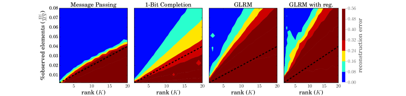
(a) *

Figure 2: The matrix completion error for Message Passing, 1-Bit matrix completion and GLRM (with and without regularization) as a function of matrix rank and portion of observed elements $|\Omega|$ for ${M}={N}=1000$. The dashed black line indicates the tentative information bottleneck.

IV Experiments

We evaluated the performance of message passing on random matrices and real-world data. In all experiments, message passing uses damping with $\lambda=.4$, $T=200$ iterations and uniform priors ${{p}^{{{{X}}}}}_{{m},{k}}(1)={{p}^{{{{Y}}}}}_{{k},{n}}(1)=.5$. This also means that if the channel is symmetric – that is ${{p}^{{{{O}}}}}(1\mid 1)={{p}^{{{{O}}}}}(0\mid 0)>.5$ – the approximate MAP reconstruction $\widehat{{{{Z}}}}$ does not depend on ${{p}^{{{{O}}}}}$, and we could simply use ${{p}^{{{{O}}}}}_{{m},{n}}(1\mid 1)={{p}^{{{{O}}}}}_{{m},{n}}(1\mid 1)=c$ for any $c>.5$. The only remaining hyper-parameters are rank $K$ and maximum number of iterations $T$.

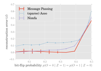
Figure 3: Comparison of message passing and NIMFA for Boolean matrix factorization

IV-A Random Matrices

Matrix Factorization. We compared our method against binary matrix factorization method of Zhang et al. (2007), which was implemented by NIMFA (Zitnik and Zupan, 2012) as well as (sparse) Asso of Miettinen et al. (2006). Here, all methods receive the correct ${K}$ as input.

Figure 3 compares the reconstruction error of different methods at different noise levels. The results are for $1000\times 1000$ random matrices of rank ${K}=5$ where ${{{X}}}$ and ${{{Y}}}$ were uniformly sampled from binary matrices. The results for different $K$ show a similar trend. The reconstruction error is

$${d}({{{Z}}},\widehat{{{{Z}}}})\quad\overset{\text{def}}{=}\quad\frac{1}{{M}{N}}\sum_{{m},{n}}|{{Z}}_{{m},{n}}-\widehat{{{Z}}}_{{m},{n}}|.$$ (11)

The results suggests that message passing and NIMFA are competitive, with message passing performing better at higher noise levels. The experiments were repeated $10$ times for each point. The small variance of message passing performance at low noise-levels is due to the multiplicity of symmetric MAP solutions, and could be resolved by performing decimation, albeit at a computational cost. We speculate that the symmetry breaking of higher noise levels help message passing choose a fixed point, which results in lower variance. Typical running times for a single matrix in this setting are 2, 15 and 20 seconds for NIMFA, message passing and sparse Asso respectively.

Despite being densely connected, at lower levels of noise, BP often converges within the maximum number of iterations. The surprisingly good performance of BP, despite the large number of loops, is because most factors have a weak influence on many of their neighboring variables. This effectively limits the number of influential loops in the factor-graph; see Appendix C for more.

Matrix Completion. The advantage of message passing to its competition is more evident in matrix “completion” problem, where the complexity of BP grows with the number of observed elements, rather than the size of matrix $Z$. We can “approximate” a lower-bound on the number of observed entries $|\Omega|=MN(1-{{p}^{{{{O}}}}}(\mathrm{null}))$ required for recovering ${{{Z}}}$ by

$$|\Omega|\ >\ {K}({M}+{N}-\log({K})+1)+\mathcal{O}(\log({K})).$$ (12)

To derive this approximation, we briefly sketch an information theoretic argument. Note that the total number of ways to define a Boolean matrix ${{{Z}}}\in\{0,1\}^{{M}\times{N}}$ of rank ${K}$ is $\frac{2^{{K}({M}+{N})}}{{K}!}$, where the nominator is the number of different ${{{X}}}$ and ${{{Y}}}$ matrices and ${K}!$ is the irrelevant degree of freedom in choosing the permutation matrix ${{{U}}}$, such that ${{{Z}}}=({{{X}}}\bullet{{{U}}})\bullet({{{U}}}^{T}\bullet{{{Y}}})$. The logarithm of this number, using Sterling’s approximation, is the r.h.s. of Equation 12, lower-bounding the number of bits required to recover ${{{Z}}}$, in the absence of any noise. Note that this is assuming that any other degrees of freedom in producing ${{{Z}}}$ grows sub-exponentially with $K$ – i.e., is absorbed in the additive term $\mathcal{O}(\log({K}))$. This approximation also resembles the $\mathcal{O}({K}{N}\mathrm{polylog}({N}))$ sample complexity for various real-domain matrix completion tasks (e.g.,  Candes and Plan, 2010; Keshavan et al., 2010).

Figure 2 compares message passing against GLRM and 1-Bit matrix completion. In all panels of Figure 2, each point represents the average reconstruction error for random $1000\times 1000$ Boolean matrices. For each choice of observation percentage $\frac{|\Omega|}{MN}$ and rank ${K}$, the experiments were repeated $10$ times. The dashed black line is the information theoretic approximate lower-bound of Equation 12. This result suggests that message passing outperforms both of these methods and remains effective close to this bound.

Figure 2 also suggests that, when using message passing, the transition from recoverability to non-recoverability is sharp. Indeed the variance of the reconstruction error is always close to zero, but in a small neighborhood of the dashed black line.

IV-B Real-World Applications

This section evaluates message passing on two real-world applications. While there is no reason to believe that the real-world matrices must necessarily decompose into low-rank Boolean factors, we see that Boolean completion using message passing performs well in comparison with other methods that assume Real factors.

TABLE I: Matrix completion performance for MovieLense dataset.

		time (sec)	binary	observed percentage of available ratings
		min-max	input?	1%	5%	10%	20%	50%	95%
1M-dataset	message passing	2-43	Y	56%	65%	67%	69%	71%	71%
	GLRM (ordinal hinge)	2-141	N	48%	65%	68%	70%	71%	72%
	GLRM (logistic)	4-90	Y	46%	63%	63%	63%	63%	62%
100K-dataset	message passing	0-2	Y	52%	60%	63%	65%	67%	70%
	GLRM (ordinal hinge)	0-2	N	48%	58%	63%	67%	69%	70%
	GLRM (logistic)	0-2	Y	45%	50%	62%	63%	62%	67%
	1-bit completion	30-500	Y	50%	53%	61%	65%	70%	72%

IV-B1 MovieLens Dataset

We applied our message passing method to MovieLens-1M and MovieLens-100K dataset as an application in collaborative filtering. The Movie-Lense-1M dataset contains 1 million ratings from 6000 users on 4000 movies (i.e., $1/24$ of all the ratings are available). The ratings are ordinals 1-5. Here we say a user is “interested” in the movie iff her rating is above the global average of ratings. The task is to predict this single bit by observing a random subset of the available user$\times$movie rating matrix. For this, we use $\alpha\in(0,1)$ portion of the $10^{6}$ ratings to predict the one-bit interest level for the remaining ($1-\alpha$ portion of the) data-points. Note that here $|\Omega|=\frac{\alpha\,M\,{N}}{24}$. The same procedure is applied to the smaller Movie-Lens-100K dataset. The reason for including this dataset was to compare message passing performance with 1-Bit matrix completion that does not scale as well.

We report the results using GLRM with logistic and ordinal hinge loss (Rennie and Srebro, 2005) and quadratic regularization of the factors. Here, only GLRM with ordinal hinge loss uses actual ratings (non-binary) to predict the ordinal ratings which are then thresholded.

Table I reports the run-time and test error of all methods for $K=2$, using different $\alpha\in\{.01,.05,.1,.2,.5,.95\}$ portion of the available ratings. It is surprising that only using one bit of information per rating, message passing and 1-bit completion are competitive with ordinal hinge loss that benefits from the full range of ordinal values. The results also suggest that when only few observations are available (e.g., $\alpha=.01$), message passing performs better than all other methods. With larger number of binary observations, 1-bit completion performs slightly better than message passing, but it is orders of magnitude slower. Here, the variance in the range of reported times in Table I is due to variance in the number of observed entries – i.e., $\alpha=.01$ often has the smallest run-time.

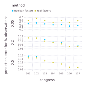
Figure 4: The prediction error using Boolean matrix completion (by message passing) versus using GLRM with hinge loss for binary matrix completion using real factors. Each panel has a different observed percentage of entries $\frac{|\Omega|}{MN}\in\{.05,.2,.5\}$. Here the horizontal axis identifies senator$\times$issue matrices and the y-axis is the average error in prediction of the unobserved portion of the (yes/no) votes.

IV-B2 Reconstructing Senate Voting Records

We applied our noisy completion method to predict the (yes/no) senate votes during 1989-2003 by observing a randomly selected subset of votes. This dataset contains $7$ Boolean matrices (corresponding to voting sessions for $101^{st}-107^{th}$ congress), where a small portion of entries are missing. For example the first matrix is a $634\times 103$ Boolean matrix recording the vote of 102 senators on $634$ topics plus the outcome of the vote (which we ignore).

Figure 4 compares the prediction accuracy in terms of reconstruction error Equation 11 of message passing and GLRM (with hinge loss or binary predictions) for the best choice of ${K}\in\{1,\ldots,10\}$ on each of 7 matrices. In each case we report the prediction accuracy on the unobserved entries, after observing $\frac{|\Omega|}{MN}\in\{5\%,20\%,50\%\}$ of the votes. For sparse observations ($\frac{|\Omega|}{MN}=.05$), the message passing error is almost always half of the error when we use real factors. With larger number of observations, the methods are comparable, with GLRM performing slightly better.

Conclusion & Future Work

This paper introduced a simple message passing technique for approximate Boolean factorization and noisy matrix completion. While having a linear time complexity, this procedure favorably compares with the state-of-the-art in Boolean matrix factorization and completion. In particular, for matrix completion with few entries, message passing significantly outperforms the existing methods that use real factors. This makes message passing a useful candidate for collaborative filtering in modern applications involving large datasets of sparse Boolean observations.

Boolean matrix factorization with modular arithmetic, replaces the logical OR operation with exclusive-OR, only changing one of the factor types (i.e., type ${\mathsf{g}}$) in our graphical model. Therefore both min-sum and sum-product message passing can also be applied to this variation. The similarity of this type of Boolean factorization to LDPC codes, suggests that one may be able to use noisy matrix completion as an efficient method of communication over a noisy channel, where the data is preprocessed to have low-rank matrix form and a few of its entries are then transmitted through the noisy channel. This is particularly interesting, as both the code and its parity checks are transmitted as a part of the same matrix. We leave this promising direction to future work.

Appendix A Detailed Derivation of Simplified BP Messages

The sum of the factors in the factor-graph of Figure 1 is

$$\sum_{{m},{k}}{\mathsf{h}}_{{m},{k}}({{X}}_{{m},{k}})+\sum_{{n},{k}}{\mathsf{h}}_{{n},{k}}({{Y}}_{{n},{k}})+$$

$$\sum_{{m},{n},{k}}{\mathsf{f}}_{{m},{n},{k}}({{X}}_{{m},{n},{k}},{{Y}}_{{m},{n},{k}},{{W}}_{{m},{n},{k}})+$$

$$\sum_{{m},{n}}{\mathsf{g}}_{{m},{n}}(\{{{W}}_{{m},{n},{k}}\}_{k})$$ (13)

$$= \sum_{{m},{n}}\log({{p}^{{{{X}}}}}({{X}}_{{m},{k}}))+\sum_{{n},{k}}\log({{p}^{{{{Y}}}}}({{Y}}_{{k},{n}}))+$$

$$\sum_{{m},{n},{k}}\mathbb{I}({{W}}_{{m},{n},{k}}={{X}}_{m,{k}}\wedge{{Y}}_{{k},{n}})+$$

$$\sum_{{m},{n}}\log\big{(}{{p}^{{{{O}}}}}_{{m},{n}}({{O}}_{{m},{n}}\mid\bigvee_{{k}}{{W}}_{{m},{n},{k}})\big{)}$$ (14)

$$= \sum_{{m},{n}}\log({{p}^{{{{X}}}}}({{X}}_{{m},{k}}))+\sum_{{n},{k}}\log({{p}^{{{{Y}}}}}({{Y}}_{{k},{n}}))+$$

$$\sum_{{m},{n}}\log\big{(}{{p}^{{{{O}}}}}_{{m},{n}}({{O}}_{{m},{n}}\mid\bigvee_{{k}}{{X}}_{m,{k}}\wedge{{Y}}_{{k},{n}})\big{)}$$ (15)

$$= \log({p}({{{X}}},{{{Y}}}\mid{{{O}}}))$$ (16)

where in Equation 14 we replaced each factor with its definition. Equation 15 combines the two last terms of Equation 14, which is equivalent to marginalizing out ${{{W}}}$. The final result of Equation 16 is the log-posterior of Equation 5.

Since the original MAP inference problem of $\arg_{{{{X}}},{{{Y}}}}\max\;{p}({{{X}}},{{{Y}}}\mid{{{O}}})$ is equivalent to $\arg_{{{{X}}},{{{Y}}}}\max\;\log({p}({{{X}}},{{{Y}}}\mid{{{O}}}))$, our objective is to perform max-sum inference over this factor-graph, finding an assignment that maximizes the summation of Equation 13

We perform this max-sum inference using Belief Propagation (BP). Applied to a factor-graph, BP involves message exchange between neighboring variable and factor nodes. Two most well-known variations of BP are sum-product BP for marginalization and max-product or max-sum BP for MAP inference. Here, we provide some details on algebraic manipulations that lead to the simplified form of max-sum BP message updates of Equation 6. Section A-A obtains the updates Equation 6c and Equation 6d in our algorithm and Section A-B reviews the remaining message updates of Equation 6

A-A Variable-to-Factor Messages

Consider the binary variable ${{X}}_{{m},{k}}\in\{0,1\}$ in the graphical model of Figure 1. Let $\mathfrak{m}_{{{X}}_{{m},{k}}\to{\mathsf{f}}_{{m},{n},{k}}}({{X}}_{{m},{k}}):\{0,1\}\to\Re$ be the message from variable ${{X}}_{{m},{k}}$ to the factor ${\mathsf{f}}_{{m},{n},{k}}$ in this factor-graph. Note that this message contains two assignments for ${{X}}_{{m},{k}}=0$ and ${{X}}_{{m},{k}}=1$. As we show here, in our simplified updates this message is represented by $\hat{\Phi}_{{m},{n},{k}}$. In the max-sum BP, the outgoing message from any variable to a neighboring factor is the sum of all incoming messages, except for the message from the receiving factor – i.e.,

$$\mathfrak{m}_{{{X}}_{{m},{k}}\to{\mathsf{f}}_{{m},{n},{k}}}({{X}}_{{m},{k}})^{(\mathrm{t+1})}=\mathfrak{m}_{{\mathsf{h}}_{{m},{k}}\to{{X}}_{{m},{k}}}({{X}}_{{m},{k}})^{(\mathrm{t})}$$

$$+\,\sum_{{n}^{\prime}\neq{n}}\mathfrak{m}_{{\mathsf{f}}_{{m},{n}^{\prime},{k}}\to{{X}}_{{m},{k}}}({{X}}_{{m},{k}})^{(\mathrm{t})}\;+\;c$$ (17)

What matters in BP messages is the difference between the message $\mathfrak{m}_{{{X}}_{{m},{k}}\to{\mathsf{f}}_{{m},{n},{k}}}({{X}}_{{m},{k}})$ assignment for ${{X}}_{{m},{k}}=1$ and ${{X}}_{{m},{k}}=0$ (note the constant $c$ in Equation 17). Therefore we can use a singleton message value that capture this difference instead of using a message over the binary domain – i.e.,

$$\hat{\Phi}_{{m},{n},{k}}=\mathfrak{m}_{{{X}}_{{m},{k}}\to{\mathsf{f}}_{{m},{n},{k}}}(1)-\mathfrak{m}_{{{X}}_{{m},{k}}\to{\mathsf{f}}_{{m},{n},{k}}}(0)$$ (18)

This is equivalent to assuming that the messages are normalized so that $\mathfrak{m}_{{{X}}_{{m},{k}}\to{\mathsf{f}}_{{m},{n},{k}}}(0)=0$. We will extensively use this normalization assumption in the following. By substituting Equation 17 in Equation 18 we get the simplified update of Equation 6c

$$\hat{\Phi}_{{m},{n},{k}}^{(\mathrm{t+1})} =\bigg{(}\mathfrak{m}_{{\mathsf{h}}_{{m},{k}}\to{{X}}_{{m},{k}}}(1)^{(\mathrm{t})}\;+\;\sum_{{n}^{\prime}\neq{n}}\mathfrak{m}_{{\mathsf{f}}_{{m},{n}^{\prime},{k}}\to{{X}}_{{m},{k}}}(1)^{(\mathrm{t})}(1)\bigg{)}$$

$$-\bigg{(}\mathfrak{m}_{{\mathsf{h}}_{{m},{k}}\to{{X}}_{{m},{k}}}(0)^{(\mathrm{t})}\;+\sum_{{n}^{\prime}\neq{n}}\mathfrak{m}_{{\mathsf{f}}_{{m},{n}^{\prime},{k}}\to{{X}}_{{m},{k}}}(0)^{(\mathrm{t})}\bigg{)}$$

$$=\bigg{(}\mathfrak{m}_{{\mathsf{h}}_{{m},{k}}\to{{X}}_{{m},{k}}}(1)^{(\mathrm{t})}-\mathfrak{m}_{{\mathsf{h}}_{{m},{k}}\to{{X}}_{{m},{k}}}(0)^{(\mathrm{t})}\bigg{)}$$

$$+\sum_{n^{\prime}\neq n}\bigg{(}\mathfrak{m}_{{\mathsf{f}}_{{m},{n}^{\prime},{k}}\to{{X}}_{{m},{k}}(1)^{(\mathrm{t})}}-\mathfrak{m}_{{\mathsf{f}}_{{m},{n}^{\prime},{k}}\to{{X}}_{{m},{k}}}(0)^{(\mathrm{t})}\bigg{)}$$

$$=\log\bigg{(}\frac{{{p}^{{{{X}}}}}_{{m},{k}}(1)}{{{p}^{{{{X}}}}}_{{m},{k}}(0)}\bigg{)}+\sum_{{n}^{\prime}\neq{n}}\;\Phi_{{m},{n}^{\prime},{k}}^{(\mathrm{t})}$$

and we used the fact that

$$\Phi_{{m},{n}^{\prime},{k}}={\mathfrak{m}_{{\mathsf{f}}_{{m},{n}^{\prime},{k}}\to{{X}}_{{m},{k}}}(1)^{(\mathrm{t})}}\;-\;{\mathfrak{m}_{{\mathsf{f}}_{{m},{n}^{\prime},{k}}\to{{X}}_{{m},{k}}}(0)^{(\mathrm{t})}}$$

$$\log\bigg{(}\frac{{{p}^{{{{X}}}}}_{{m},{k}}(1)}{{{p}^{{{{X}}}}}_{{m},{k}}(0)}\bigg{)}={\mathsf{h}}_{{m},{k}}(1)-{\mathsf{h}}_{{m},{k}}(0).$$

The messages $\hat{\Psi}_{{m},{n},{k}}$ from the variables ${{Y}}_{{n},{k}}$ to ${\mathsf{f}}_{{m},{n},{k}}$ is obtain similarly. The only remaining variable-to-factor messages in the factor-graph of Figure 1 are from auxiliary variables ${{W}}_{{m},n,k}$ to neighboring factors. However, since each variable ${{W}}_{{m},{n},k}$ has exactly two neighboring factors, the message from ${{W}}_{{m},{n},{k}}$ to any of these factors is simply the incoming message from the other factor – that is

$$\mathfrak{m}_{{{W}}_{{m},{n},{k}}\to{\mathsf{g}}_{{m},{n}}}({{W}}_{{m},{n},{k}})=\mathfrak{m}_{{\mathsf{f}}_{{m},{n},{k}}\to{{W}}_{{m},{n},{k}}}({{W}}_{{m},{n},{k}})$$

$$\mathfrak{m}_{{\mathsf{g}}_{{m},{n}}\to{{W}}_{{m},{n},{k}}}({{W}}_{{m},{n},{k}})=\mathfrak{m}_{{{W}}_{{m},{n},{k}}\to{\mathsf{f}}_{{m},{n},{k}}}({{W}}_{{m},{n},{k}})$$ (19)

A-B Factor-to-Variable Messages

The factor-graph of Figure 1 has three types of factors. We obtain the simplified messages from each of these factors to their neighboring variables in the following sections.

A-B1 Local Factors

The local factors are $\{{\mathsf{h}}_{{m},k}\}_{{m},{k}}$ and $\{{\mathsf{h}}_{n,k}\}_{{n},{k}}$, each of which is only connected to a single variable. The unnormalized message, leaving these factors is identical to the factor itself. We already used the normalized messages from these local factors to neighboring variables in Equation 19 – i.e., ${\mathsf{h}}_{{m},k}(1)-{\mathsf{h}}_{{m},k}(0)$ and ${\mathsf{h}}_{{n},k}(1)-{\mathsf{h}}_{{n},k}(0)$, respectively.

A-B2 Constraint Factors

The constraint factors $\{{\mathsf{f}}_{{m},{n},{k}}\}_{{m},{n},{k}}$ ensure $\forall_{{m},{n},{k}}{{W}}_{{m},{n},{k}}={{X}}_{{m},{k}}\wedge{{Y}}_{{n},{k}}$. Each of these factors has three neighboring variables. In max-sum BP the message from a factor to a neighboring variable is given by the sum of that factor and incoming messages from its neighboring variables, except for the receiving variable, max-marginalized over the domain of the receiving variable. Here we first calculate the messages from a constraint factor to ${{X}}_{{m},{k}}$ (or equivalently ${{Y}}_{{n},{k}}$) variables in (1). In (2) we derive the simplified messages to the auxiliary variable ${{W}}_{{m},{n},{k}}$.

(1) according to max-sum BP equations the message from the factor ${\mathsf{f}}_{{m},{n},{k}}$ to variable ${{{X}}_{{m},{k}}}$ is

$$\mathfrak{m}_{{\mathsf{f}}_{{m},{n},{k}}\to{{X}}_{{m},{k}}}({{X}}_{{m},{k}})^{(\mathrm{t+1})}=$$

$$\max_{{{W}}_{{m},{n},{k}},{{Y}}_{{n},{k}}}\bigg{(}{\mathsf{f}}_{{m},{n},{k}}({{X}}_{{m},{k}},{{W}}_{{m},{n},{k}},{{Y}}_{{n},{k}})$$

$$+\,\mathfrak{m}_{{{Y}}_{{n},{k}}{\mathsf{f}}_{{m},{n},{k}}\to(}{{Y}}_{{n},{k}})^{(\mathrm{t})}+\,\mathfrak{m}_{{{W}}_{{m},{n},{k}}\to{\mathsf{f}}_{{m},{n},{k}}}({{W}}_{{m},{n},{k}})^{(\mathrm{t})}\bigg{)}$$

For notational simplicity we temporarily use the shortened version of the above

$$\mathfrak{m}_{1}^{\prime}({{X}})=\max_{{{W}},{{Y}}}{\mathsf{f}}({{X}},{{W}},{{Y}})\;+\mathfrak{m}_{2}({{Y}})+\mathfrak{m}_{3}({{W}})$$ (20)

where

$$\mathfrak{m}_{1}({{X}})=\mathfrak{m}_{{{X}}_{{m},{k}}\to{\mathsf{f}}_{{m},{n},{k}}}({{X}}_{{m},{k}})$$

$$\mathfrak{m}^{\prime}_{1}({{X}})=\mathfrak{m}_{{\mathsf{f}}_{{m},{n},{k}}\to{{X}}_{{m},{k}}}({{X}}_{{m},{k}})$$

$$\mathfrak{m}_{2}({{Y}})=\mathfrak{m}_{{{Y}}_{{n},{k}}\to{\mathsf{f}}_{{m},{n},{k}}}({{Y}}_{{n},{k}})$$

$$\mathfrak{m}^{\prime}_{2}({{Y}})=\mathfrak{m}_{{\mathsf{f}}_{{m},{n},{k}}\to{{Y}}_{{n},{k}}}({{Y}}_{{n},{k}})$$

$$\mathfrak{m}_{3}({{W}})=\mathfrak{m}_{{{W}}_{{m},{n},{k}}\to{\mathsf{f}}_{{m},{n},{k}}}({{W}}_{{m},{n},{k}})$$

$$\mathfrak{m}^{\prime}_{3}({{W}})=\mathfrak{m}_{{\mathsf{f}}_{{m},{n},{k}}\to{{W}}_{{m},{n},{k}}}({{W}}_{{m},{n},{k}}),$$

that is we use $\mathfrak{m}(.)$ to denote the incoming messages to the factor and $\mathfrak{m}^{\prime}(.)$ to identify the outgoing message.

If the constraint ${\mathsf{f}}({{X}},{{Y}},{{W}})=\mathbb{I}({{W}}={{X}}\wedge{{Y}})$ is not satisfied by an assignment to ${{X}},{{Y}}$ and ${{W}}$, it evaluates to $-\infty$, and therefore it does not have any effect on the outgoing message due to the $\max$ operation. Therefore we should consider the $\max_{{{W}},{{Y}}}$ only over the assignments that satisfy ${\mathsf{f}}(.)$.

Here, ${{X}}$ can have two assignments; for ${{X}}=1$, if ${{Y}}=1$, then ${{W}}=1$ is enforced by ${\mathsf{f}}(.)$, and if ${{Y}}=0$ then ${{W}}=0$. Therefore Equation 20 for ${{X}}=1$ becomes

$$\mathfrak{m}_{1}^{\prime}(1)=\max(\mathfrak{m}_{2}(1)+\mathfrak{m}_{3}(1),\mathfrak{m}_{2}(0)+\mathfrak{m}_{3}(0))$$ (21)

For ${{X}}=0$, we have ${{W}}=0$, regardless of ${{Y}}$ and the update of Equation 20 reduces to

$$\mathfrak{m}^{\prime}_{1}(0)\; =\;\max(\mathfrak{m}_{2}(1)+\mathfrak{m}_{3}(0),\mathfrak{m}_{2}(0)+\mathfrak{m}_{3}(0)\}$$ (22)

$$=\mathfrak{m}_{3}(0)+\max\{\mathfrak{m}2(0),\mathfrak{m}2(1)\}$$

Assuming the incoming messages are normalized such that $\mathfrak{m}_{3}(0)=\mathfrak{m}_{2}(0)=0$ and denoting

$$\hat{\Psi}_{{m},{n},{k}}=\mathfrak{m}_{{{Y}}_{{n},{k}}\to{\mathsf{f}}_{{m},{n},{k}}}(1)-\mathfrak{m}_{{{Y}}_{{n},{k}}\to{\mathsf{f}}_{{m},{n},{k}}}(0)=\mathfrak{m}_{2}(1)$$

and

$$\Gamma_{{m},{n},{k}}=\mathfrak{m}_{{{W}}_{{m},{n},{k}}\to{\mathsf{f}}_{{m},{n},{k}}}(1)-\mathfrak{m}_{{{W}}_{{m},{n},{k}}\to{\mathsf{f}}_{{m},{n},{k}}}(0)=\mathfrak{m}_{3}(1)$$

the difference of Equation 21 and Equation 22 gives the normalized outgoing message of Equation 6a

$$\Phi_{{m},{n},{k}}= \mathfrak{m}^{\prime}_{1}(1)-\mathfrak{m}^{\prime}_{1}(0)=\max(\Gamma_{{m},{n},{k}}+\hat{\Psi}_{{m},{n},{k}},0)$$

$$- \max(0,\hat{\Psi}_{{m},{n},{k}})$$ (23)

The message of Equation 6b from the constraint ${\mathsf{f}}_{{m},{n},{k}}$ to ${{Y}}_{{n},{k}}$ is obtained in exactly the same way.

(2) The max-sum BP message from the constraint factor ${\mathsf{f}}_{{m},{n},{k}}$ to the auxiliary variable ${{W}}_{{m},{n},{k}}$ is

$$\mathfrak{m}_{{\mathsf{f}}_{{m},{n},{k}}\to{{W}}_{{m},{n},{k}}}({{W}}_{{m},{n},{k}})^{(\mathrm{t+1})}=$$

$$\max_{{{X}}_{{m},{k}},{{Y}}_{{n},{k}}}\big{(}{\mathsf{f}}_{{m},{n},{k}}({{X}}_{{m},{k}},{{W}}_{{m},{n},{k}},{{Y}}_{{n},{k}})+$$

$$\mathfrak{m}_{{{Y}}_{{n},{k}}\to{\mathsf{f}}_{{m},{n},{k}}}({{Y}}_{{n},{k}})^{(\mathrm{t})}+\mathfrak{m}_{{{X}}_{{m},{k}}\to{\mathsf{f}}_{{m},{n},{k}}}({{W}}_{{m},{n},{k}})^{(\mathrm{t})}\big{)}$$

Here, again we use the short notation

$$\mathfrak{m}^{\prime}_{3}({{W}})=\max_{{{X}},{{Y}}}{\mathsf{f}}({{X}},{{W}},{{Y}})\;+\mathfrak{m}_{1}({{X}})+\mathfrak{m}_{2}({{Y}})$$ (24)

and consider the outgoing message $\mathfrak{m}^{\prime}({{W}})$ for ${{W}}=1$ and ${{W}}=0$. If ${{W}}=1$, we know that ${{X}}={{Y}}=1$. This is because otherwise the factor ${\mathsf{f}}$ evaluates to $-\infty$. This simplifies Equation 24 to

$$\mathfrak{m}_{3}^{\prime}(1)=\mathfrak{m}_{1}(1)+\mathfrak{m}_{2}(1)$$

For ${{W}}=0$, either ${{X}}=0$, or ${{Y}}=0$ or both. This means

$$\mathfrak{m}^{\prime}_{3}(0)=\max( \mathfrak{m}_{1}(0)+\mathfrak{m}_{2}(1),\mathfrak{m}+1(1)+\mathfrak{m}_{2}(0),$$

$$\mathfrak{m}_{1}(0)+\mathfrak{m}_{2}(0))$$

Assuming the incoming messages were normalized, such that $\mathfrak{m}_{2}(0)=\mathfrak{m}_{1}(0)=0$, the normalized outgoing message $\hat{\Gamma}_{{m},{n},{k}}=\mathfrak{m}_{3}(1)-\mathfrak{m}_{3}(0)$ simplifies to

$$\hat{\Gamma}_{{m},{n},{k}} =\mathfrak{m}_{1}(1)+\mathfrak{m}_{2}(1)-\max(0,\mathfrak{m}_{1}(1),\mathfrak{m}_{2}(1))$$

$$=\min(\mathfrak{m}_{1}(1)+\mathfrak{m}_{2}(1),\mathfrak{m}_{1}(1),\mathfrak{m}_{2}(1))$$

$$=\min(\hat{\Phi}_{{m},{n},{k}}+\hat{\Psi}_{{m},{n},{k}},\hat{\Phi}_{{m},{n},{k}},\hat{\Psi}_{{m},{n},{k}})$$

A-C Likelihood Factors

At this point we have derived all simplified message updates of Equation 6, except for the message $\Gamma_{{m},{n},{k}}$ from factors ${\mathsf{g}}_{m,n}$ to the auxiliary variables ${{W}}_{{m},{n},{k}}$ (Equation 6f). These factors encode the likelihood term in the factor-graph.

The naive form of max-sum BP for the messages leaving this factor to each of ${K}$ neighboring variables $\{{{W}}_{{m},{n},{k}}\}_{1\leq{k}\leq{K}}$ is

$$\mathfrak{m}_{{\mathsf{g}}_{{m},{n}}\to{{W}}_{{m},{n},{k}}}({{W}}_{{m},{n},{k}})^{(\mathrm{t+1})}=$$ (25)

$$\max_{\{{{W}}_{{m},{n},\ell}\}_{\ell\neq{k}\}}}\bigg{(}{\mathsf{g}}_{{m},{n}}(\{{{W}}_{{m},{n},{\ell^{\prime}}}\}_{\ell^{\prime}})+$$

$$\sum_{{k}^{\prime}\neq{k}}\mathfrak{m}_{{{W}}_{{m},{n},{k}^{\prime}}\to{\mathsf{g}}_{{m},{n}}}({{W}}_{{m},{n},{k}^{\prime}})^{(\mathrm{t})}\bigg{)}$$

However, since ${\mathsf{g}}(.)$ is a high-order factor (i.e., depends on many variables), this naive update has an exponential cost in ${K}$. Fortunately, by exploiting the special form of ${\mathsf{g}}(.)$, we can reduce this cost to linear in ${K}$.

In evaluating ${\mathsf{g}}(\{{{W}}_{{m},{n},{k}}\}_{k})$ two scenarios are conceivable:

1. at least one of ${{W}}_{{m},{n},1},\ldots,{{W}}_{{m},{n},{K}}$ is non-zero – that is $\bigvee_{{k}}{{W}}_{{m},{n},{k}}=1$ and ${\mathsf{g}}({{W}}_{{m},{n},{k}})$ evaluates to ${{p}^{{{{O}}}}}_{{m},{n}}({{O}}_{{m},{n}}\mid 1)$.

2. $\bigvee_{{k}}{{W}}_{{m},{n},{k}}=0$ and ${\mathsf{g}}({{W}}_{{m},{n},{k}})$ evaluates to ${{p}^{{{{O}}}}}_{{m},{n}}({{O}}_{{m},{n}}\mid 0)$.

We can divide the maximization of Equation 25 into two separate maximization operations over sets of assignments depending on the conditioning above and select the maximum of the two.

For simplicity, let $\mathfrak{m}_{1}({{W}}_{1}),\ldots,\mathfrak{m}_{K}({{W}}_{K})$ denote $\mathfrak{m}_{{{W}}_{{m},{n},1}\to{\mathsf{g}}_{{m},{n}}}({{W}}_{{m},{n},1})^{(\mathrm{t})},\ldots,\mathfrak{m}_{{{W}}_{{m},{n},{K}}\to{\mathsf{g}}_{{m},{n}}}({{W}}_{{m},{n},{K}})^{(\mathrm{t})}$ respectively. W.L.O.G., let us assume the objective is to calculate the outgoing message to the first variable $\mathfrak{m}^{\prime}_{1}({{W}}_{1})=\mathfrak{m}_{{\mathsf{g}}_{{m},{n}}\to{{W}}_{{m},{n},1}}({{W}}_{{m},{n},1})^{(\mathrm{t+1})}$. Let us rewrite Equation 25 using this notation:

$$\mathfrak{m}^{\prime}_{1}({{W}}_{1})=\max_{{{W}}_{2}\ldots{{W}}_{{K}}}\big{(}{\mathsf{g}}_{{m},{n}}(\{{{W}}_{k}\})+\sum_{{k}^{\prime}>1}\mathfrak{m}_{{k}^{\prime}}({{W}}_{{k}^{\prime}})\big{)}$$

For ${{W}}_{1}=1$, regardless of assignments to ${{W}}_{2},\ldots,{{W}}_{K}$, we have $\bigvee_{{k}}{{W}}_{{m},{n},{k}}=1$ and therefore the maximization above simplifies to

$$\mathfrak{m}^{\prime}_{1}(1) =\max_{{{W}}_{2}\ldots{{W}}_{{K}}}\big{(}\log({{p}^{{{{O}}}}}_{{m},{n}}({{O}}_{{m},{n}}\mid 1))\sum_{{k}^{\prime}>1}\mathfrak{m}_{{k}^{\prime}}({{W}}_{{k}^{\prime}})\big{)}$$

$$=\log({{p}^{{{{O}}}}}_{{m},{n}}({{O}}_{{m},{n}}\mid 1))+\sum_{{k}^{\prime}>1}\max(\mathfrak{m}_{{k}^{\prime}}(0),\mathfrak{m}_{{k}^{\prime}}(1)).$$

For ${{W}}_{1}=0$, if $\forall_{{k}^{\prime}>1}{{W}}_{{k}^{\prime}}=0$ then ${\mathsf{g}}(\{{{W}}_{k}\})$ evaluates to $\log({{p}^{{{{O}}}}}_{{m},{n}}({{O}}_{{m},{n}}\mid 0)$, and otherwise it evaluates to $\log({{p}^{{{{O}}}}}_{{m},{n}}({{O}}_{{m},{n}}\mid 1)$. We need to choose the maximum over these two cases. Note that in the second case we have to ensure at least one of the remaining variables is non-zero – i.e., $\exists_{{k}^{\prime}>1}{{W}}_{{k}^{\prime}}=1$. In the following update to enforce this constraint we use

$${k}^{*}=\arg_{{k}^{\prime}>1}\max\mathfrak{m}_{{k}^{\prime}}(1)-\mathfrak{m}_{{k}^{\prime}}(0)$$ (26)

to get

$$\mathfrak{m}^{\prime}_{1}(0)=\max\bigg{(} \log({{p}^{{{{O}}}}}_{{m},{n}}({{O}}_{{m},{n}}\mid 0)+\sum_{{k}^{\prime}>1}\mathfrak{m}_{{k}^{\prime}}(0)\;,\;$$

$$\log({{p}^{{{{O}}}}}_{{m},{n}}({{O}}_{{m},{n}}\mid 1)+\mathfrak{m}_{{k}^{*}}+$$

$$\sum_{{k}^{\prime}>1,{k}^{\prime}\neq{k}^{*}}\max(\mathfrak{m}_{{k}^{\prime}}(0),\mathfrak{m}_{{k}^{\prime}}(1))\bigg{)}$$

where, choosing ${{W}}_{{k}^{*}}=1$ maximizes the second case (where at least one ${{W}}_{{k}^{\prime}}$ for ${k}^{\prime}>1$ is non-zero).

As before, let us assume that the incoming messages are normalized such that $\forall_{{k}^{\prime}}\mathfrak{m}_{{k}^{\prime}}(0)=0$, and therefore $\hat{\Gamma}_{{m},{n},{k}^{\prime}}=\mathfrak{m}_{{k}^{\prime}}(1)$. The normalized outgoing message is

$$\Gamma_{{m},{n},1}=\mathfrak{m}^{\prime}_{1}(1)-\mathfrak{m}^{\prime}(0)=\log({{p}^{{{{O}}}}}_{{m},{n}}({{O}}_{{m},{n}}\mid 1))$$

$$+\sum_{{k}^{\prime}>1}\max(0,\mathfrak{m}_{{k}^{\prime}}(1))-$$

$$\max\bigg{(}\log({{p}^{{{{O}}}}}_{{m},{n}}({{O}}_{{m},{n}}\mid 0),\log({{p}^{{{{O}}}}}_{{m},{n}}({{O}}_{{m},{n}}\mid 1)+\mathfrak{m}_{{k}^{*}}$$

$$+\sum_{{k}^{\prime}>1,{k}^{\prime}\neq{k}^{*}}\max(0,\mathfrak{m}_{{k}^{\prime}}(1))\bigg{)}$$

$$=\min\bigg{(}\log({{p}^{{{{O}}}}}_{{m},{n}}({{O}}_{{m},{n}}\mid 1))-\log({{p}^{{{{O}}}}}_{{m},{n}}({{O}}_{{m},{n}}\mid 0)$$

$$+\sum_{{k}^{\prime}>1}\max(0,\mathfrak{m}_{{k}^{\prime}}(1)),\max(-\mathfrak{m}_{{k}^{*}}(1),0)\bigg{)}$$

$$=\min\bigg{(}\sum_{{k}^{\prime}>1}\max(0,\hat{\Gamma}_{{m},{n},{k}^{\prime}}^{(\mathrm{t})})$$

$$+\log\bigg{(}\frac{{{p}^{{{{O}}}}}_{{m},{n}}({{O}}_{{m},{n}}\mid 1)}{{{p}^{{{{O}}}}}_{{m},{n}}({{O}}_{{m},{n}}\mid 0)}\bigg{)},\max(0,-\max_{{k}>1}\hat{\Gamma}_{{m},{n},{k}^{\prime}}^{(\mathrm{t})})\bigg{)}$$

where in the last step we used the definition of factor ${\mathsf{g}}$ and Equation 26 that defines $\mathfrak{m}_{{k}^{*}}(1)$. This produces the simplified form of BP messages for the update Equation 6f in our algorithm.

Appendix B Marginal-MAP

While the message passing for MAP inference approximates the “jointly” optimal assignment to ${{{X}}}$ and ${{{Y}}}$ in the Bayesian setting, the marginals ${p}({{X}}_{{m},{k}}\mid{{{O}}})$ and ${p}({{X}}_{{k},{n}}\mid{{{O}}})$ are concerned with optimal assignments to “individual” ${{X}}_{{m},{k}}$ and ${{Y}}_{{k},{n}}$ for each ${m},{n}$ and ${k}$. Here again, message passing can approximate the log-ratio of these marginals.

We use the function ${\phi}(a)=\log(1+\exp(a))$ and its inverse ${\phi}^{-1}(b)=\log(\exp(b)-1)$ in the following updates for marginalization.

$$\Phi_{{m},{n},{k}}^{(\mathrm{t+1})}:={\Gamma_{{m},{n},{k}}^{(\mathrm{t})}+\hat{\Psi}_{{m},{n},{k}}^{(\mathrm{t})}}\,-$$

$$\,\log\big{(}1+\exp(\hat{\Psi}_{{m},{n},{k}}^{(\mathrm{t})})+\exp(\hat{\Phi}_{{m},{n},{k}}^{(\mathrm{t})})\big{)}$$

$$\Psi_{{m},{n},{k}}^{(\mathrm{t+1})}:={\Gamma_{{m},{n},{k}}^{(\mathrm{t})}+\hat{\Phi}_{{m},{n},{k}}^{(\mathrm{t})}}\,-$$

$$\,\log\big{(}1+\exp(\hat{\Phi}_{{m},{n},{k}}^{(\mathrm{t})}+\exp(\hat{\Psi}_{{m},{n},{k}}^{(\mathrm{t})})\big{)}$$

$$\hat{\Phi}_{{m},{n},{k}}^{(\mathrm{t+1})}:=\log\bigg{(}\frac{{{p}^{{{{X}}}}}_{{m},{k}}(1)}{{{p}^{{{{X}}}}}_{{m},{k}}(0)}\bigg{)}+\sum_{{n}^{\prime}\neq{n}}\;\Phi_{{m},{n}^{\prime},{k}}^{(\mathrm{t})}$$

$$\hat{\Psi}_{{m},{n},{k}}^{(\mathrm{t+1})}:=\log\bigg{(}\frac{{{p}^{{{{Y}}}}}_{{n},{k}}(1)}{{{p}^{{{{Y}}}}}_{{n},{k}}(0)}\bigg{)}+\sum_{{m}^{\prime}\neq{m}}\;\Psi_{{m}^{\prime},{n},{k}}^{(\mathrm{t})}$$

$$\hat{\Gamma}_{{m},{n},{k}}^{(\mathrm{t+1})}:=\hat{\Phi}_{{m},{n},{k}}^{(\mathrm{t})}+\hat{\Psi}_{{m},{n},{k}}^{(\mathrm{t})}$$

$$\Gamma_{{m},{n},{k}}^{(\mathrm{t+1})}:=\sum_{{k}^{\prime}\neq{k}}{\phi}(\hat{\Gamma}_{{m},{n},{k}^{\prime}}^{(\mathrm{t})})\,+\,\log\bigg{(}\frac{{{p}^{{{{O}}}}}_{{m},{n}}({{O}}_{{m},{n}}\mid 1)}{{{p}^{{{{O}}}}}_{{m},{n}}({{O}}_{{m},{n}}\mid 0)}\bigg{)}$$

$$-\,{\phi}\bigg{(}\phi^{-1}\big{(}\sum_{{k}^{\prime}\neq{k}}{\phi}(\hat{\Gamma}_{{m},{n},{k}^{\prime}}^{(\mathrm{t})})\big{)}$$

$$+\,\log\bigg{(}\frac{{{p}^{{{{O}}}}}_{{m},{n}}({{O}}_{{m},{n}}\mid 1)}{{{p}^{{{{O}}}}}_{{m},{n}}({{O}}_{{m},{n}}\mid 0)}\bigg{)}\bigg{)}$$

Here, again using Equation 7, we can recover ${{{X}}}$ and ${{{Y}}}$ from the marginals. However, due to the symmetry of the set of solutions, one needs to perform decimation to obtain an assignment to ${{{X}}}$ and ${{{Y}}}$. Decimation is the iterative process of running message passing then fixing the most biased variable – e.g., an ${{X}}_{{m},{k}}\ \in\ \arg_{{m},{k}}\max|\Xi_{{m},{k}}|$ – after each convergence. While a simple randomized initialization of messages is often enough to break the symmetry of the solutions in max-sum inference, in the sum-product case one has to repeatedly fix a new subset of most biased variables.

observed           original   GLRM           message passing    

(a) *

(b) *

(c) *

(d) $\rho\in\{.01,\,.02,\,.05\}$, $K=10$

(e) $K\in\{2,\,20,\,200\}$, $\rho=.02$

(f) reg.

Figure 5: Comparison of low-rank Boolean matrix completion using 1) message passing (using Boolean factors) and 2) GLRM (using real-valued factors) for ${K}=10$. The first column shows the original image (top) and the observation for $\rho=.01$ (bottom). (a) increasing numbers of observations $\rho$; (b) increasing rank ${K}$; (c) using quadratic regularization for GLRM and sparsity inducing priors ${{p}^{{{{X}}}}}_{{m},{k}}(0)={{p}^{{{{X}}}}}_{{m},{k}}(0)=.9$ for message passing. Here ${K}=20$ and $\rho=.02$ – i.e., similar to the figure (b) middle.

Appendix C Uninfluential Edges

Figure 6 shows the histogram of factor-to-variable messages $\{\hat{\Phi}_{{m},{n}}\}_{1\leq{m}{M},1\leq{n}\leq N}$ at different iterations. It suggests that a large portion of messages are close to zero. Since these are log-ratios, the corresponding probabilities are close to uniform. Uniform message over an edge in a factor-graph is equivalent to non-existing edges, which in turn reduces the number of influential loops in the factor-graph.

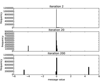
Figure 6: Histogram of BP messages $\{\hat{\Phi}_{{m},{n}}^{(\mathrm{t})}\}_{{m},{n}}$ at $t\in\{2,20,200\}$ for a random $1000\times 1000$ matrix factorization with ${K}=2$.

Appendix D Image Completion

Figure 5 is an example of completing a $1000\times 1000$ black and white image, here using message passing or GLRM. In Figure 5(a) we vary the number of observed pixels $\rho\in\{.01,\,.02,\,.05\}$ with fixed ${K}=10$ and in Figure 5(b) we vary the rank ${K}\in\{2,\,20,\,200\}$, while fixing $\rho=.02$. A visual inspection of reconstructions suggests that, since GLRM is using real factors, it can easily over-fit the observation as we increase the rank. However, the Boolean factorization, despite being expressive, does not show over-fitting behavior for larger rank values – as if the result was regularized. In Figure 5(c), we regularize both methods for ${K}=20$: for GLRM we use Gaussian priors over both ${{{X}}}$ and ${{{Y}}}$ and for message passing we use sparsity inducing priors ${{p}^{{{{X}}}}}_{{m},{k}}(0)={{p}^{{{{X}}}}}_{{m},{k}}(0)=.9$. This improves the performance of both methods. However, note that regularization does not significantly improve the results of GLRM when applied to the matrix completion task, where the underlying factors are known to be Boolean (see Figure 2(right)).

References

- Atia and Saligrama (2012) George K Atia and Venkatesh Saligrama. Boolean compressed sensing and noisy group testing. Information Theory, IEEE Transactions on, 58(3):1880–1901, 2012.
- Belohlavek et al. (2007) Radim Belohlavek, Jiří Dvořák, and Jan Outrata. Fast factorization by similarity in formal concept analysis of data with fuzzy attributes. Journal of Computer and System Sciences, 73(6):1012–1022, 2007.
- Candes and Plan (2010) Emmanuel J Candes and Yaniv Plan. Matrix completion with noise. Proceedings of the IEEE, 98(6):925–936, 2010.
- Cover and Thomas (2012) Thomas M Cover and Joy A Thomas. Elements of information theory. John Wiley & Sons, 2012.
- Davenport et al. (2014) Mark A Davenport, Yaniv Plan, Ewout van den Berg, and Mary Wootters. 1-bit matrix completion. Information and Inference, 3(3):189–223, 2014.
- Decelle et al. (2011) Aurelien Decelle, Florent Krzakala, Cristopher Moore, and Lenka Zdeborová. Asymptotic analysis of the stochastic block model for modular networks and its algorithmic applications. Physical Review E, 84(6):066106, 2011.
- Dimakis et al. (2012) Alexandros G Dimakis, Roxana Smarandache, and Pascal O Vontobel. Ldpc codes for compressed sensing. Information Theory, IEEE Transactions on, 58(5):3093–3114, 2012.
- Donoho (2006) David L Donoho. Compressed sensing. Information Theory, IEEE Transactions on, 52(4):1289–1306, 2006.
- Donoho et al. (2009) David L Donoho, Arian Maleki, and Andrea Montanari. Message-passing algorithms for compressed sensing. Proceedings of the National Academy of Sciences, 106(45):18914–18919, 2009.
- Du and Hwang (1993) Ding-Zhu Du and Frank K Hwang. Combinatorial group testing and its applications. World Scientific, 1993.
- Frey and Dueck (2007) Brendan J Frey and Delbert Dueck. Clustering by passing messages between data points. science, 315(5814):972–976, 2007.
- Gallager (1962) Robert G Gallager. Low-density parity-check codes. Information Theory, IRE Transactions on, 8(1):21–28, 1962.
- Geerts et al. (2004) Floris Geerts, Bart Goethals, and Taneli Mielikäinen. Tiling databases. In Discovery science, pages 278–289. Springer, 2004.
- Gupta et al. (2007) Rahul Gupta, Ajit A Diwan, and Sunita Sarawagi. Efficient inference with cardinality-based clique potentials. In Proceedings of the 24th international conference on Machine learning, pages 329–336. ACM, 2007.
- Jakulin et al. (2009) Aleks Jakulin, Wray Buntine, Timothy M La Pira, and Holly Brasher. Analyzing the us senate in 2003: Similarities, clusters, and blocs. Political Analysis, page mpp006, 2009.
- Kabashima et al. (2014) Yoshiyuki Kabashima, Florent Krzakala, Marc Mézard, Ayaka Sakata, and Lenka Zdeborová. Phase transitions and sample complexity in bayes-optimal matrix factorization. arXiv preprint arXiv:1402.1298, 2014.
- Keprt and Snásel (2004) Ales Keprt and Václav Snásel. Binary factor analysis with help of formal concepts. In CLA, volume 110, pages 90–101, 2004.
- Keshavan et al. (2010) Raghunandan H Keshavan, Andrea Montanari, and Sewoong Oh. Matrix completion from a few entries. Information Theory, IEEE Transactions on, 56(6):2980–2998, 2010.
- Krzakala et al. (2013) Florent Krzakala, Marc Mézard, and Lenka Zdeborová. Phase diagram and approximate message passing for blind calibration and dictionary learning. In Information Theory Proceedings (ISIT), 2013 IEEE International Symposium on, pages 659–663. IEEE, 2013.
- Kschischang et al. (2001) Frank R Kschischang, Brendan J Frey, and Hans-Andrea Loeliger. Factor graphs and the sum-product algorithm. Information Theory, IEEE Transactions on, 47(2):498–519, 2001.
- Lu et al. (2008) Haibing Lu, Jaideep Vaidya, and Vijayalakshmi Atluri. Optimal boolean matrix decomposition: Application to role engineering. In Data Engineering, 2008. ICDE 2008. IEEE 24th International Conference on, pages 297–306. IEEE, 2008.
- Maurus and Plant (2014) Samuel Maurus and Claudia Plant. Ternary matrix factorization. In Data Mining (ICDM), 2014 IEEE International Conference on, pages 400–409. IEEE, 2014.
- McDonald (2014) Roderick P McDonald. Factor analysis and related methods. Psychology Press, 2014.
- Middleton et al. (1991) Blackford Middleton, Michael Shwe, David Heckerman, Max Henrion, Eric Horvitz, Harold Lehmann, and Gregory Cooper. Probabilistic diagnosis using a reformulation of the internist-1/qmr knowledge base. Medicine, 30:241–255, 1991.
- Miettinen and Vreeken (2011) Pauli Miettinen and Jilles Vreeken. Model order selection for boolean matrix factorization. In Proceedings of the 17th ACM SIGKDD international conference on Knowledge discovery and data mining, pages 51–59. ACM, 2011.
- Miettinen et al. (2006) Pauli Miettinen, Taneli Mielikäinen, Aristides Gionis, Gautam Das, and Heikki Mannila. The discrete basis problem. In Knowledge Discovery in Databases: PKDD 2006, pages 335–346. Springer, 2006.
- Mnih and Salakhutdinov (2007) Andriy Mnih and Ruslan Salakhutdinov. Probabilistic matrix factorization. In Advances in neural information processing systems, pages 1257–1264, 2007.
- Parker et al. (2013) Jason T Parker, Philip Schniter, and Volkan Cevher. Bilinear generalized approximate message passing. arXiv preprint arXiv:1310.2632, 2013.
- Pearl (1982) Judea Pearl. Reverend bayes on inference engines: A distributed hierarchical approach. In AAAI, pages 133–136, 1982.
- Pearl (2014) Judea Pearl. Probabilistic reasoning in intelligent systems: networks of plausible inference. Morgan Kaufmann, 2014.
- Ravanbakhsh and Greiner (2014) Siamak Ravanbakhsh and Russell Greiner. Revisiting algebra and complexity of inference in graphical models. arXiv preprint arXiv:1409.7410, 2014.
- Ravanbakhsh et al. (2014) Siamak Ravanbakhsh, Reihaneh Rabbany, and Russell Greiner. Augmentative message passing for traveling salesman problem and graph partitioning. In Advances in Neural Information Processing Systems, pages 289–297, 2014.
- Rennie and Srebro (2005) Jason DM Rennie and Nathan Srebro. Loss functions for preference levels: Regression with discrete ordered labels. In Proceedings of the IJCAI multidisciplinary workshop on advances in preference handling, pages 180–186. Kluwer Norwell, MA, 2005.
- Sejdinovic and Johnson (2010) Dino Sejdinovic and Oliver Johnson. Note on noisy group testing: asymptotic bounds and belief propagation reconstruction. In Communication, Control, and Computing (Allerton), 2010 48th Annual Allerton Conference on, pages 998–1003. IEEE, 2010.
- Šingliar and Hauskrecht (2006) Tomáš Šingliar and Miloš Hauskrecht. Noisy-or component analysis and its application to link analysis. The Journal of Machine Learning Research, 7:2189–2213, 2006.
- Stockmeyer (1975) Larry J Stockmeyer. The set basis problem is NP-complete. IBM Thomas J. Watson Research Division, 1975.
- Udell et al. (2014) Madeleine Udell, Corinne Horn, Reza Zadeh, and Stephen Boyd. Generalized low rank models. arXiv preprint arXiv:1410.0342, 2014.
- Vaidya et al. (2007) Jaideep Vaidya, Vijayalakshmi Atluri, and Qi Guo. The role mining problem: finding a minimal descriptive set of roles. In Proceedings of the 12th ACM symposium on Access control models and technologies, pages 175–184. ACM, 2007.
- Weiss and Freeman (2001) Yair Weiss and William T Freeman. On the optimality of solutions of the max-product belief-propagation algorithm in arbitrary graphs. Information Theory, IEEE Transactions on, 47(2):736–744, 2001.
- Weiss et al. (2012) Yair Weiss, Chen Yanover, and Talya Meltzer. Map estimation, linear programming and belief propagation with convex free energies. arXiv preprint arXiv:1206.5286, 2012.
- Wood et al. (2012) Frank Wood, Thomas Griffiths, and Zoubin Ghahramani. A non-parametric bayesian method for inferring hidden causes. arXiv preprint arXiv:1206.6865, 2012.
- Yedidia et al. (2000) Jonathan S Yedidia, William T Freeman, Yair Weiss, et al. Generalized belief propagation. In NIPS, volume 13, pages 689–695, 2000.
- Zhang et al. (2010) Zhong-Yuan Zhang, Tao Li, Chris Ding, Xian-Wen Ren, and Xiang-Sun Zhang. Binary matrix factorization for analyzing gene expression data. Data Mining and Knowledge Discovery, 20(1):28–52, 2010.
- Zhang et al. (2007) Zhongyuan Zhang, Chris Ding, Tao Li, and Xiangsun Zhang. Binary matrix factorization with applications. In Data Mining, 2007. ICDM 2007. Seventh IEEE International Conference on, pages 391–400. IEEE, 2007.
- Zitnik and Zupan (2012) Marinka Zitnik and Blaz Zupan. Nimfa: A python library for nonnegative matrix factorization. Journal of Machine Learning Research, 13:849–853, 2012.