Could a change in magnetic field geometry cause the break in the wind-activity relation?

Abstract

Wood et al suggested that mass-loss rate is a function of X-ray flux ($\dot{M}\propto F_{x}^{1.34}$) for dwarf stars with $F_{x}\lesssim F_{x,6}\equiv 10^{6}$ erg cm^-2 s^-1. However, more active stars do not obey this relation. These authors suggested that the break at $F_{x,6}$ could be caused by significant changes in magnetic field topology that would inhibit stellar wind generation. Here, we investigate this hypothesis by analysing the stars in Wood et al’s sample that had their surface magnetic fields reconstructed through Zeeman-Doppler Imaging (ZDI). Although the solar-like outliers in the $\dot{M}$ – $F_{x}$ relation have higher fractional toroidal magnetic energy, we do not find evidence of a sharp transition in magnetic topology at $F_{x,6}$. To confirm this, further wind measurements and ZDI observations at both sides of the break are required. As active stars can jump between states with highly toroidal to highly poloidal fields, we expect significant scatter in magnetic field topology to exist for stars with $F_{x}\gtrsim F_{x,6}$. This strengthens the importance of multi-epoch ZDI observations. Finally, we show that there is a correlation between $F_{x}$ and magnetic energy, which implies that $\dot{M}$ – magnetic energy relation has the same qualitative behaviour as the original $\dot{M}$ – $F_{x}$ relation. No break is seen in any of the $F_{x}$ – magnetic energy relations.

1 Introduction

Like the Sun, low-mass stars experience mass loss through winds during their entire lives. Although the solar wind can be probed in situ, the existence of winds on low-mass stars is known indirectly, e.g., from the observed rotational evolution of stars (see Bouvier et al., 2014, and references therein). Measuring the wind rates $\dot{M}$ of cool, low-mass stars is not usually an easy task though. Although in their youth, when the stars are still surrounded by accretion discs, their winds have been detected (Kwan, Edwards & Fischer, 2007; Gómez de Castro & Verdugo, 2007), this is no longer the case after their accretion discs dissipate. The belief is that, from the dissipation of the disc onwards, winds of low-mass stars are no longer as dense, making it more difficult to detect them directly.

There have been several attempts to detect radio free-free thermal emission from the winds of low-mass stars. The lack of detection means that only upper limits in $\dot{M}$ can be derived (e.g., van den Oord & Doyle, 1997; Gaidos, Güdel & Blake, 2000; Villadsen et al., 2014). Detecting X-ray emission generated when ionised wind particles exchange charges with neutral atoms of the interstellar medium has also been considered, but again only upper limits on $\dot{M}$ could be derived (Wargelin & Drake, 2002). Other methods, involving the detection of coronal radio flares (Lim & White, 1996) or the accretion of wind material from a cool, main-sequence component to a white dwarf component (Debes, 2006; Parsons et al., 2012), have also been suggested. However, the indirect method of Wood et al. (2001) has been the most successful one, enabling estimates of $\dot{M}$ for about a dozen dwarf stars.

This method assumes that the observed excess absorption in the blue wing of the HI Lyman-$\alpha$ line is caused by the hydrogen wall that forms when the stellar wind interacts with the interstellar medium. Unfortunately, this method requires high-resolution UV spectroscopy, low HI-column density along the line-of-sight and a suitable viewing angle of the system (Wood et al., 2005b), making it difficult to estimate $\dot{M}$ for a large number of stars. Wood et al. (2002, 2005a) showed that, for dwarf stars, there seems to be a relationship between the mass-loss rate per unit surface area $A_{\star}$ and the X-ray flux $F_{x}$, for stars with $F_{x}\lesssim 10^{6}$ erg cm^-2s^-1

$$\dot{M}/A_{\star}\propto F_{x}^{1.34}.$$ (1)

Because stars, as they age, rotate more slowly and because their activity decreases with rotation, X-ray fluxes also decay with age (e.g., Guedel, 2004). Thus, the $\dot{M}$ – $F_{x}$ relation implies that stars that are younger and have larger $F_{x}$, should also have higher $\dot{M}$. This, consequently, can have important effects on the early evolution of planetary systems. For example, extrapolations using Eq. (1) suggest that the 700 Myr-Sun would have had $\dot{M}$ that is $\sim 100$ times larger than the current solar mass-loss rate $\dot{M}_{\odot}=2\times 10^{14}~{}{\rm M}_{\odot}~{}{\rm yr}^{-1}$ (Wood et al., 2005a). If this is indeed the case, this can explain the loss of the Martian atmosphere as due to erosion caused by the stronger wind of the young Sun (Wood, 2004).

However, more active stars with $F_{x}\gtrsim 10^{6}$ erg cm^-2s^-1 do not obey Eq. (1) – their derived $\dot{M}$ are several orders of magnitude smaller than what Eq. (1) predicts (Wood et al., 2005a, 2014). What could cause the change in wind characteristics at $F_{x}\sim 10^{6}$ erg cm^-2s^-1? Wood et al. (2005a) hypothesised that the stars to the right of the “wind dividing line” (WDL; i.e., with $F_{x}\gtrsim 10^{6}$ erg cm^-2s^-1) have a concentration of spots at high latitudes, as recognised in Doppler Imaging studies (e.g., Strassmeier, 2009), which could influence the magnetic field geometry of the star. They argue that these objects might possess a strong dipole component (or strong toroidal fields, Wood & Linsky 2010) “that could envelope the entire star and inhibit stellar outflows”.

In this Letter, we investigate the hypothesis that solar-type stars to the right of the WDL should have a distinct magnetic field topology compared to the stars to the left of the WDL. For that, we select stars in Wood et al’s sample that have large-scale surface magnetic fields previously reconstructed through Zeeman-Doppler Imaging (ZDI). In our analysis, only the large-scale surface fields are considered and we cannot assess if something happening at a smaller magnetic scale can affect the $\dot{M}$ – $F_{x}$ relation.

2 Magnetic field reconstruction

Our sample consists of 7 objects (Table 1) out of 12 dwarf stars (not considering the Sun) in Wood et al’s sample.

Table 1: Properties of the stars considered in this work. Rotation periods $P_{\rm rot}$ were derived in the associated ZDI work (references in Table 2), while the remaining values are from Wood 2004, Wood & Linsky 2010, Wood et al. 2014. Note that $F_{x}$, $\dot{M}$ and the magnetic maps are not necessarily derived at the same observational epoch.

Star	Sp.	$R_{\star}$	Prot	$F_{x}$	$\dot{M}$
ID	Type	$(R_{\odot})$	(days)	($10^{5}$ erg/s/cm2)	$(\dot{M}_{\odot})$
EV Lac	M3.5V	$0.35$	$4.4$	$130$	$1.0$
$\xi$ Boo A	G8V	$0.83$	$5.6$	$17$	$0.5$
$\pi^{1}$ UMa	G1.5V	$0.95$	$5.0$	$17$	$0.5$
$\epsilon$ Eri	K1V	$0.78$	$10.3$	$5.6$	$30.0$
$\xi$ Boo B	K4V	$0.61$	$10.3$	$4.1$	$4.5$
61 Cyg A	K5V	$0.68$	$34.2$	$1.0$	$0.5$
$\epsilon$ Ind	K5V	$0.75$	$37.2$	$0.72$	$0.5$
Sun	G2V	$1.00$	$25.0$	$0.32^{a}$	$1.0$

^aWithin its cycle, the Sun’s X-ray luminosity varies from $\simeq 0.27$ to $4.7\times 10^{27}$ erg s^-1 (Peres et al., 2000), corresponding to $F_{x}=4.4\times 10^{4}$ and $7.7\times 10^{5}$ erg cm^-2s^-1, respectively. For consistency, we chose however to use the same value as used in Wood et al. (2014), which is more representative of the Sun at minimum.

The large-scale magnetic fields were observationally-derived through the ZDI technique (Morin et al. 2008; Morgenthaler et al. 2012; Jeffers et al. 2014, Petit et al in prep, Boro Saikia et al in prep, Boisse et al in prep). This technique consists of reconstructing the stellar surface magnetic field based on a series of circularly polarised spectra (Donati & Brown, 1997). In its most recent implementation, ZDI solves for the radial $B_{r}$, meridional $B_{\theta}$ and azimuthal $B_{\varphi}$ components of the stellar magnetic field, expressed in terms of spherical harmonics and their colatitude-derivatives (Donati et al., 2006b)

$$B_{r}(\theta,\varphi)=\sum_{\rm lm}\alpha_{\rm lm}P_{\rm lm}e^{im\varphi}\,,$$ (2)

$$B_{\theta}(\theta,\varphi)=\sum_{\rm lm}\left[\frac{\beta_{\rm lm}}{l+1}\frac{{\rm d}P_{\rm lm}}{{\rm d}\theta}+\frac{\gamma_{\rm lm}}{l+1}\frac{im}{\sin\theta}P_{\rm lm}\right]e^{im\varphi}\,,$$ (3)

$$B_{\varphi}(\theta,\varphi)=-\sum_{\rm lm}\left[\frac{\beta_{\rm lm}}{l+1}\frac{im}{\sin\theta}P_{\rm lm}-\frac{\gamma_{\rm lm}}{l+1}\frac{{\rm d}P_{\rm lm}}{{\rm d}\theta}\right]e^{im\varphi}\,,$$ (4)

where $\alpha_{\rm lm}$, $\beta_{\rm lm}$, $\gamma_{\rm lm}$ are the coefficients that provide the best fit to the spectropolarimetric data and $P_{\rm lm}\equiv P_{\rm lm}(\cos\theta)$ is the associated Legendre polynomial of degree $l$ and order $m$.

To quantify the magnetic characteristics of the stars in our sample, we compute the following quantities (Table 2):
$\bullet$ The average squared magnetic field (i.e., proportional to the magnetic energy): $\langle B^{2}\rangle=\frac{1}{4\pi}\int(B_{r}^{2}+B_{\theta}^{2}+B_{\varphi}^{2})\sin\theta d\theta d\varphi$.
$\bullet$ The average squared poloidal component of the magnetic field $\langle B_{\rm pol}^{2}\rangle$ and its fraction $f_{\rm pol}={\langle B_{\rm pol}^{2}\rangle}/{\langle B^{2}\rangle}$. To calculate $\langle B_{\rm pol}^{2}\rangle$, we neglect terms with $\gamma_{\rm lm}$ in Eqs. (3) and (4).
$\bullet$ The axisymmetric part of the poloidal energy $\langle B_{\rm axi}^{2}\rangle$ and its fraction with respect to the poloidal component $f_{\rm axi}={\langle B_{\rm axi}^{2}\rangle}/{\langle B_{\rm pol}^{2}\rangle}$. To calculate $\langle B_{\rm axi}^{2}\rangle$, we restrict the sum of the poloidal magnetic field energy to orders $m=0$, $m<l/2$.
$\bullet$ The average squared toroidal component of the magnetic field $\langle B_{\rm tor}^{2}\rangle=\langle B^{2}\rangle-\langle B_{\rm pol}^{2}\rangle$ and its fraction $f_{\rm tor}=1-f_{\rm pol}$.
$\bullet$ The average squared dipolar component of the magnetic field $\langle B_{\rm dip}^{2}\rangle$ and its fraction $f_{\rm dip}={\langle B_{\rm dip}^{2}\rangle}/{\langle B^{2}\rangle}$. To calculate $\langle B_{\rm dip}^{2}\rangle$, we restrict the sum of the total magnetic field energy (i.e., including the three components of $\mathbf{B}$) to degree $l=1$.

Table 2: Magnetic properties of our sample. EV Lac, $\xi$ Boo A and $\epsilon$ Eri had their properties averaged over multi epochs (App. A).

Star	$\langle B^{2}\rangle$	$\langle B_{\rm pol}^{2}\rangle$	$\langle B_{\rm tor}^{2}\rangle$	$\langle B_{\rm axi}^{2}\rangle$	$\langle B_{\rm dip}^{2}\rangle$	$f_{\rm pol}$	$f_{\rm tor}$	$f_{\rm axi}$	$f_{\rm dip}$	Reference for surface
ID	(G2)	(G2)	(G2)	(G2)	(G2)					magnetic map
EV Lacb	$3.6\times 10^{5}$	$3.4\times 10^{5}$	$1.7\times 10^{4}$	$1.0\times 10^{5}$	$2.5\times 10^{5}$	$0.95$	$0.05$	$0.31$	$0.72$	Morin et al. (2008)
$\xi$ Boo Ab	$1.8\times 10^{3}$	$6.6\times 10^{2}$	$1.1\times 10^{3}$	$3.4\times 10^{2}$	$1.2\times 10^{3}$	$0.37$	$0.63$	$0.51$	$0.43$	Morgenthaler et al. (2012)
$\pi^{1}$ UMa	$1.1\times 10^{3}$	$2.0\times 10^{2}$	$8.9\times 10^{2}$	$3.3\times 10^{1}$	$7.4\times 10^{2}$	$0.18$	$0.82$	$0.16$	$0.68$	Petit et al. (in prep)
$\epsilon$ Erib	$2.7\times 10^{2}$	$2.0\times 10^{2}$	$7.5\times 10^{1}$	$7.8\times 10^{1}$	$2.0\times 10^{2}$	$0.72$	$0.28$	$0.40$	$0.75$	Jeffers et al. (2014)
$\xi$ Boo B	$4.0\times 10^{2}$	$2.7\times 10^{2}$	$1.3\times 10^{2}$	$7.3\times 10^{1}$	$1.8\times 10^{2}$	$0.68$	$0.32$	$0.27$	$0.45$	Petit et al. (in prep)
61 Cyg A	$4.5\times 10^{1}$	$3.9\times 10^{1}$	$5.7\times 10^{0}$	$8.2\times 10^{-1}$	$8.6\times 10^{0}$	$0.87$	$0.13$	$0.02$	$0.19$	Boro Saikia et al. (in prep)
$\epsilon$ Ind	$5.8\times 10^{2}$	$5.6\times 10^{2}$	$2.0\times 10^{1}$	$2.8\times 10^{2}$	$3.3\times 10^{2}$	$0.96$	$0.04$	$0.51$	$0.56$	Boisse et al. (in prep)

Similarly to the Sun, it has been recognised that stellar magnetism can evolve on a yearly timescale, with some stars exhibiting complete magnetic cycles. Three of the objects in our sample, namely EV Lac, $\xi$ Boo A and $\epsilon$ Eri, have multi-epoch reconstructed surface maps. For these stars, $f_{\rm pol}$, $f_{\rm axi}$, $f_{\rm dip}$ and $\langle B^{2}\rangle$, which are shown in Table 2, were averaged over multiple observing epochs (see Appendix A). We note that, as the observations are not done at regular time intervals, the time the star spends in a given ‘magnetic state’ might not be well represented by this simple average. However, we believe that this approach is a better representation of the magnetic characteristic for each of these stars over the choice of one single-epoch map, in particular when the star-to-star differences are comparable to the year-to-year (i.e., amplitude) variations that stars exhibit (more important in the most active stars).

3 Magnetic fields as the cause of the break in the $\dot{M}$ – $F_{x}$ relation

One proposed idea for the break in the $\dot{M}$ – $F_{x}$ relation for the most active stars is that stars that are to the right of the WDL have surface magnetic field topologies that are significantly different, with either stronger dipolar (Wood et al., 2005a) or toroidal fields (Wood & Linsky, 2010), that partially inhibit the outflow of the stellar wind, giving rise to reduced $\dot{M}$. To verify the first hypothesis, we compute $\langle B_{\rm dip}^{2}\rangle$ and $f_{\rm dip}$ for all the stars in our sample (Table 2). We do not find any particular evidence that stars to the right of the WDL, namely $\pi^{1}$ UMa, $\xi$ Boo A and EV Lac, have dipolar magnetic fields whose characteristics are remarkably different from the remaining stars in our sample.

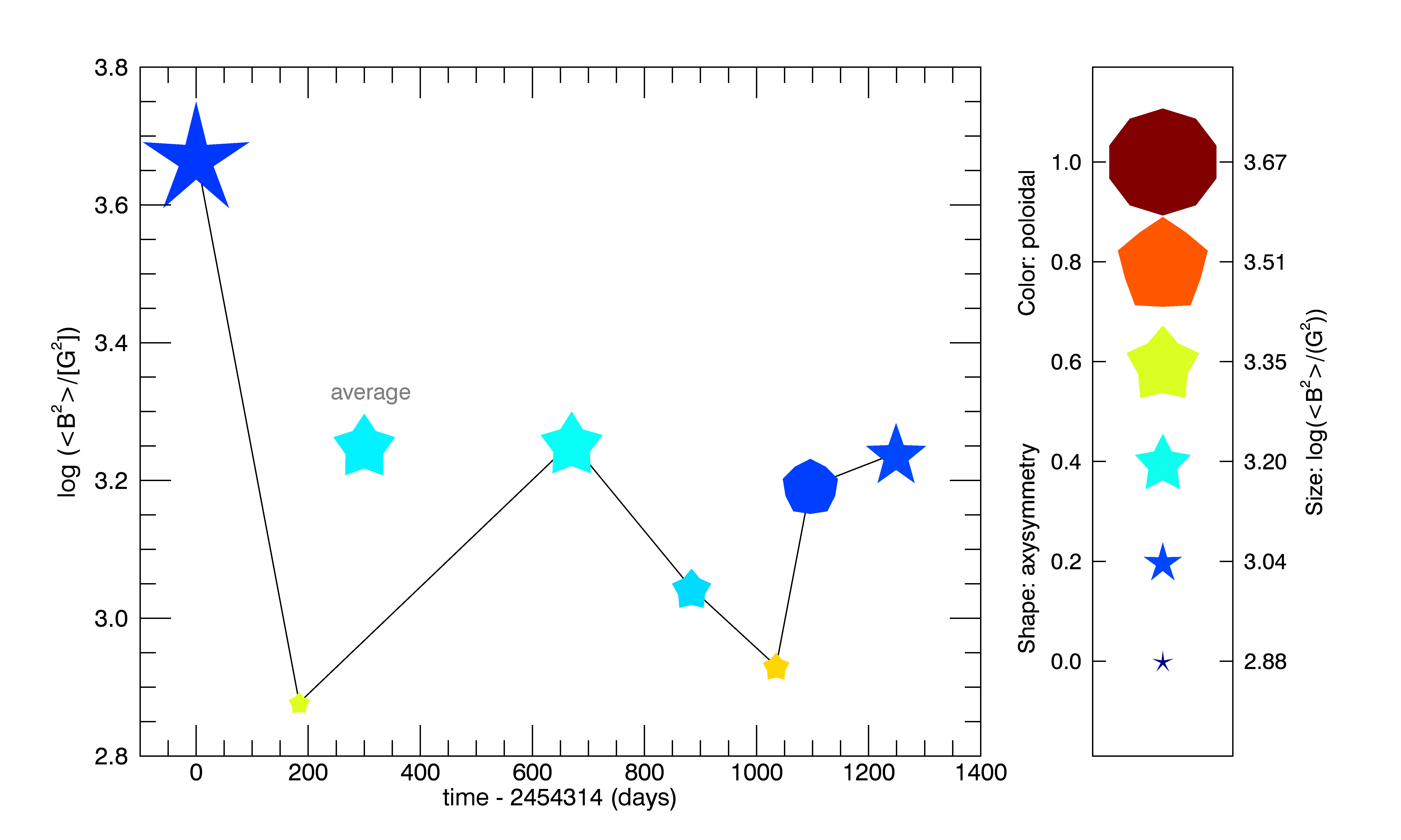
Figure 3: Evolution of the magnetic field properties of $\xi$ Boo A, according to multi-epoch magnetic field reconstructions from Morgenthaler et al. (2012). A better representation of the magnetic field property is calculated as average over the observed epochs (see text). We believe this approach is a better representation of the magnetic characteristic of the star over the choice of one single-epoch map. The same approach is employed for all the stars in our sample with multi-epoch observations, namely EV Lac and $\epsilon$ Eri. The solid line is a connector and does not represent any particular fit to the data.

Fig. 1 presents a similar version of Wood et al’s diagram ($\dot{M}/A_{\star}$ versus $F_{x}$) showing only the stars for which we have reconstructed surface fields. The symbols are as in Fig. 3 of Donati & Landstreet (2009), in which their sizes are proportional to $\log\langle B^{2}\rangle$, their colours are related to $f_{\rm pol}$, and their shapes to $f_{\rm axi}$ (see caption of figure). EV Lac is included in this plot for completeness but it is not considered in the analysis that follows. It has been argued that EV Lac could be a discrepant data point in the wind-activity relation because it is the least solar-like star in the sample (Wood, 2004). Indeed, it has been revealed that the magnetism of active M dwarf stars, like EV Lac, has striking differences from solar-like objects, both in intensity and geometry (Donati et al., 2006a, 2008; Reiners & Basri, 2007; Reiners, Basri & Browning, 2009; Morin et al., 2008, 2010). Note that, except for EV Lac, our objects have Rossby numbers $\rm Ro>0.1$, where $\rm Ro$ is defined as the ratio between the convective turnover timescale to the rotation period of the star ($\rm Ro$ compiled by Vidotto et al. 2014a). Therefore, none of our solar-type stars are in the X-ray saturated regime (Pizzolato et al., 2003).

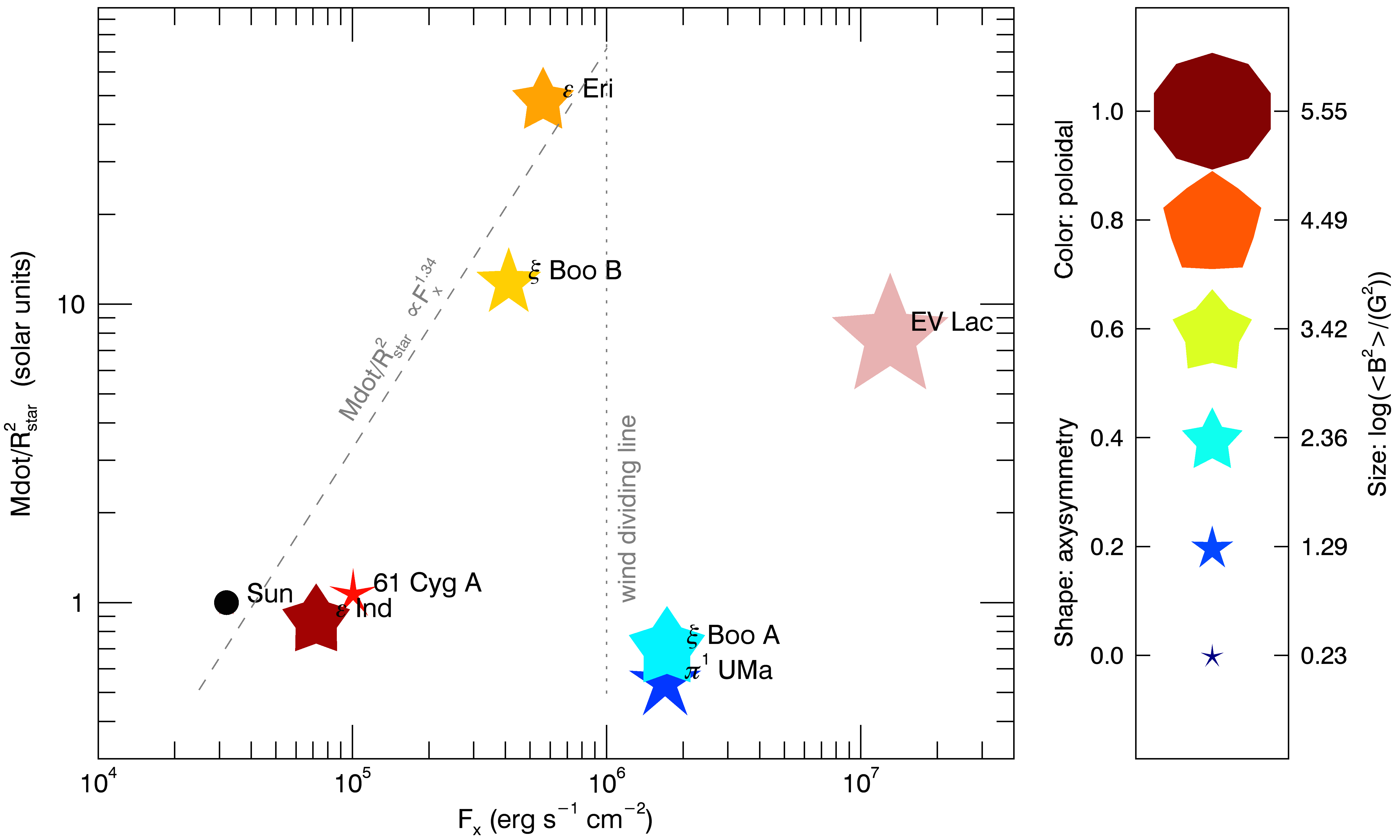
Figure 1: Mass-loss rates per surface area versus X-ray fluxes showing only the stars for which we have reconstructed surface fields. Symbol sizes are proportional to $\log\langle B^{2}\rangle$, their colours indicate the fractional poloidal energy (ranging from deep red for purely poloidal field $f_{\rm pol}=1$ to blue for purely toroidal field $f_{\rm pol}=0$), and their shapes indicate the fraction of axisymmetry of the poloidal component (ranging from a decagon for purely axisymmetric field $f_{\rm axi}=1$ to a point-shaped star for $f_{\rm axi}=0$). The $\dot{M}$ – $F_{x}$ relation (Eq. 1) is shown as a dashed line and the WDL at $F_{x}=10^{6}$ erg cm^-2s^-1 is shown as a dotted line. The Sun (filled black circle) is shown for comparison.

Table 3: Slope of the ordinary least square fits to the logarithm of our data (i.e., $y\propto x^{\rm slope}$).

y(x)	$F_{x}(\langle B_{\rm tor}^{2}\rangle)$	$F_{x}(\langle B_{\rm pol}^{2}\rangle)$	$F_{x}(\langle B_{\rm dip}^{2}\rangle)$	$F_{x}(\langle B^{2}\rangle)$
slope	$0.65\pm 0.06$	$0.47\pm 0.05$	$0.50\pm 0.03$	$0.55\pm 0.04$

Fig. 1 shows no evidence that $\dot{M}$ and $f_{\rm axi}$ (symbol shape) are related, indicating that the axisymmetry of the poloidal field cannot explain the wind-activity relation nor its break. In the Sun, $\dot{M}$ and $f_{\rm axi}$ also seem to be unrelated. The solar dipolar field, nearly aligned with the Sun’s rotation axis (and therefore nearly axisymmetric) at minimum activity phase, increasingly tilts towards the equator as the cycle approaches activity maximum (DeRosa, Brun & Hoeksema, 2012), decreasing therefore $f_{\rm axi}$. In spite of the cycle variation of $f_{\rm axi}$ in the Sun, the solar wind mass-loss rates remains largely unchanged (Wang, 2010).

What stands out in Fig. 1 is that solar-type stars with larger toroidal fractional fields (bluer) are concentrated to the right of the WDL. With the limited number of stars with both ZDI and wind measurements, there is no evidence at present for a sharp transition in magnetic topology across the WDL. Instead, the concentration of stars with dominantly toroidal fields to the right of the WDL reflects a trend towards more strongly toroidal fields with increasing $F_{x}$, which is in turn associated with rapid rotation. Petit et al. (2008) showed that, as stellar rotation increases, solar-type stars tend to have higher fraction of toroidal fields (symbols becoming increasingly bluer in diagrams such as the one expressed in Fig. 1; see also Fig. 3 in Donati & Landstreet 2009). Since rotation is linked to activity, it is not surprising that $\pi^{1}$ UMa and $\xi$ Boo A, the most active and rapidly rotating solar-type stars in our sample, are the ones with the largest fraction of toroidal fields. To confirm our findings, it is essential to perform further wind measurements and ZDI observations of more stars at both sides of the break.

We note also that if instead of plotting $F_{x}$ in the $x$-axis of Fig. 1, we plotted $\langle B_{\rm tor}^{2}\rangle$, this plot would present the same general property: $\dot{M}/A_{\star}$ that increases with $\langle B_{\rm tor}^{2}\rangle$ for the least active stars and then a break in this relation for $\pi^{1}$ UMa and $\xi$ Boo A, with the break occurring somewhere between $\langle B_{\rm tor}^{2}\rangle\sim 200$ and $800$ G². The similar characteristics between $\dot{M}/A_{\star}$ vs $F_{x}$ and $\dot{M}/A_{\star}$ vs $\langle B_{\rm tor}^{2}\rangle$ is because $\langle B_{\rm tor}^{2}\rangle$ is correlated to $F_{x}$, as shown in Fig. 2 (this figure includes EV Lac). Because $\langle B_{\rm tor}^{2}\rangle$ and $\langle B_{\rm pol}^{2}\rangle$ are correlated (See et al., 2015), correlations between $F_{x}$ and $\langle B_{\rm pol}^{2}\rangle$ or $\langle B^{2}\rangle$ also exist (see Table 3). No break is seen in any of the $F_{x}$ – magnetic energy relations. Because magnetism and X-ray flux evolve on $\sim$yearly timescales, intrinsic variability is expected to increase the spread in all the relations in Table 3, further reinforcing the importance of multi-epoch ZDI observations.

Another important point to consider is that very active stars can jump between states with highly toroidal fields and mostly poloidal fields (Petit et al. 2009; Morgenthaler et al. 2012; Boro Saikia et al. 2015). Therefore, if the high fraction of toroidal magnetic fields is related to the break on the $\dot{M}$ – $F_{x}$ relation, there may be some significant scatter in magnetic field topology on the right of the WDL. E.g., during $\sim$ 5 yr of observations, the fractional toroidal field of $\xi$ Boo A varied between $f_{\rm tor}\simeq 33\%$ to $81\%$, with an average of $63\%$, giving this star a blueish color in Fig. 1 (Appendix A). If this star were observed only during an epoch where its field is dominantly poloidal, the trend that stars to the right of the WDL are more toroidal (bluer) would not be recovered. This further strengthens the need of multi-epoch ZDI observations (cf. Section 2).

Assuming that a change in magnetic field topology is such that it will significantly affect the mass-loss rates of stellar winds, it would still take on the order of a year (depending on the size of the astrosphere) for stellar winds to propagate out into the astrosphere boundary, where the Ly-$\alpha$ photons are absorbed. Therefore, simultaneous derivations of mass-loss rate (through Ly-$\alpha$ absorption) and magnetic field topology (through ZDI) are likely not going to be linked to each other. It would, nevertheless, be interesting to monitor both Ly-$\alpha$ absorption and magnetic topologies to see whether variations of the latter mimic those of the former with a $\sim 1$ yr delay.

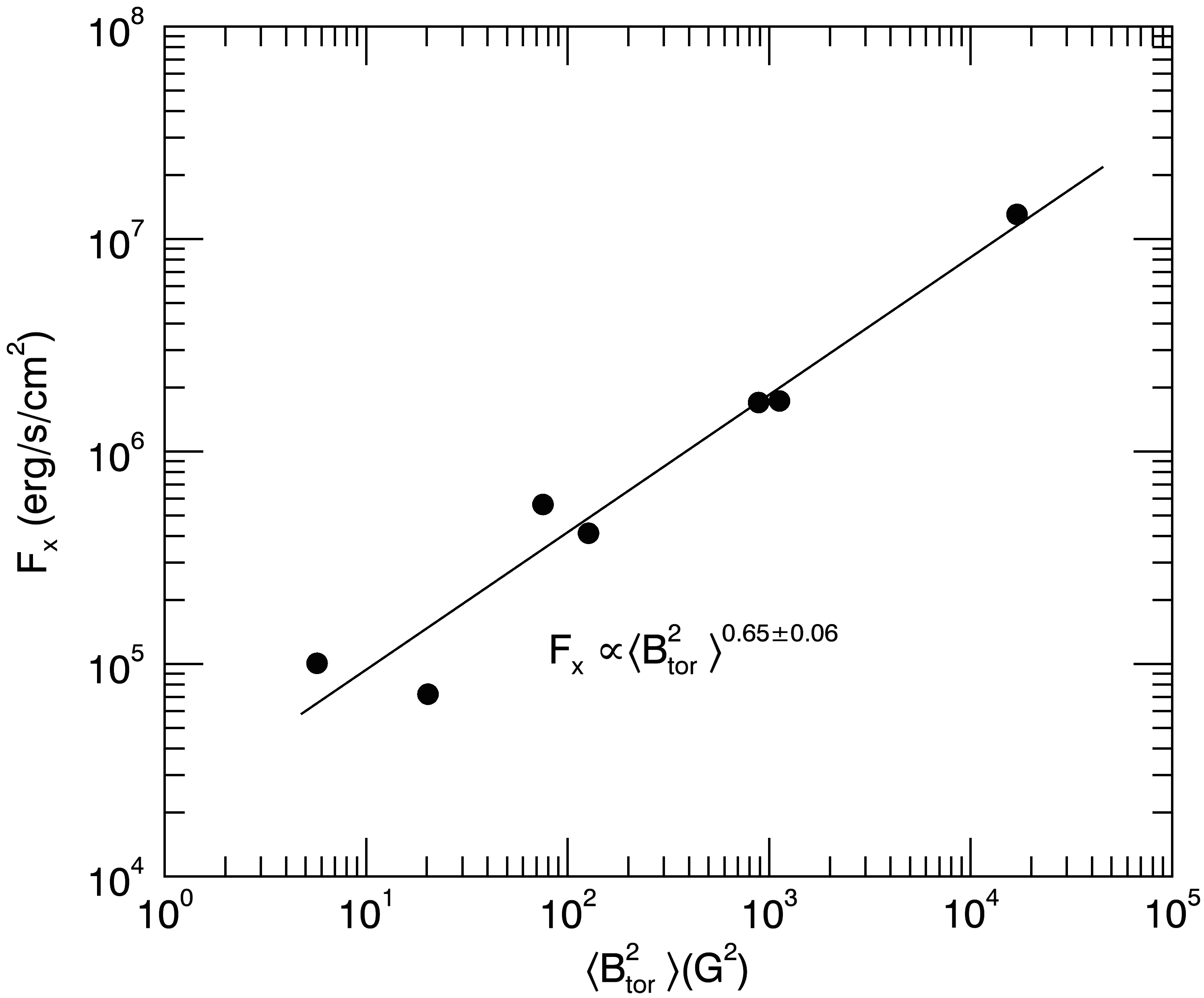
Figure 2: Relation between $F_{x}$ and $\langle B_{\rm tor}^{2}\rangle$ does not show a break at $F_{x}\sim 10^{6}$ erg cm^-2s^-1. Solid line is a power-law fit the data. Because $\langle B_{\rm tor}^{2}\rangle$ and $\langle B_{\rm pol}^{2}\rangle$ are correlated (See et al., 2015), correlations between $F_{x}$ and $\langle B_{\rm pol}^{2}\rangle$ or $\langle B^{2}\rangle$ also exist (see Table 3).

4 Conclusions and Discussion

In this letter, we have investigated if stellar magnetic fields could be the cause of the break in the wind-activity ($\dot{M}$ – $F_{x}$) relation, for stars with $F_{x}\gtrsim 10^{6}$ erg cm^-2s^-1 (Wood et al., 2005a). Our sample consisted of stars observed by Wood et al that also had observationally-derived large-scale magnetic fields (Morin et al. 2008; Morgenthaler et al. 2012; Jeffers et al. 2014, Petit et al in prep, Boro Saikia et al in prep, Boisse et al in prep).

Wood et al. (2005a) and Wood & Linsky (2010) suggested that the break in the $\dot{M}$ – $F_{x}$ relation seen for the most active stars could be caused by the presence of strong dipolar or toroidal fields that would inhibit the wind generation. In our analysis, we did not find any particular evidence that the dipolar field characteristics (or the degree of axisymmetry of the poloidal field) change at the WDL. We found that solar-type stars to the right of the WDL (namely $\xi$ Boo A and $\pi^{1}$ UMa) have higher fractional toroidal fields (blueish points in Fig. 1), but no break or sharp transition is found (Fig. 2, Petit et al. 2008).

We also showed that there is a correlation between $F_{x}$ and magnetic energy (Table 3), which implies that $\dot{M}$ – magnetic energy relation has the same general properties as the original $\dot{M}$ – $F_{x}$ relation (i.e., a positive correlation for $F_{x}\lesssim 10^{6}$ erg cm^-2s^-1, followed by a break). Contrary to the $\dot{M}$ – $F_{x}$ relation, no break at the WDL is seen in the $F_{x}$ – magnetic energy relations.

We note that very active stars can jump between states with highly toroidal fields and mostly poloidal fields (Petit et al. 2009; Morgenthaler et al. 2012; Boro Saikia et al. 2015). If magnetic fields are actually affecting stellar winds (i.e., the high fraction of toroidal fields is related to the break in the $\dot{M}$ – $F_{x}$ relation), there may be some significant scatter in magnetic field topology on the right of the WDL, even for a given star observed at various phases of its magnetic cycle.

We finally add that the break in the $\dot{M}$ – $F_{x}$ relation found by Wood et al. (2005a) is at odds with some theoretical works on stellar winds and empirically-derived relations used to compute outflow rates ($\dot{M}_{\rm CME}$) of coronal mass ejections (CMEs). The time-dependent stellar wind models of Holzwarth & Jardine (2007); See et al. (2014); Johnstone et al. (2015) predict a different (in general, weaker) dependence of $\dot{M}$ with $F_{x}$ than that of Eq. (1) and do not predict a sharp decrease in $\dot{M}$ for stars to the right of the WDL. These models use empirical data on rotation, wind temperature, density and magnetic field strength to constrain theoretical wind scenarios. They are, however, limited to one or two dimensions and cannot, therefore, incorporate the 3D nature of stellar magnetic fields. 3D stellar wind studies that incorporates observed stellar magnetic maps have been carried out but they are currently not time-dependent (Cohen et al., 2010; Vidotto et al., 2012, 2014b; Jardine et al., 2013).

Other theoretical works suggested that CMEs could be the dominant form of mass loss for active stars (Aarnio, Matt & Stassun, 2012; Drake et al., 2013; Osten & Wolk, 2015). These works predicted that $\dot{M}_{\rm CME}\gtrsim 100\dot{M}_{\odot}$ for active solar-like stars, in contradiction to the results found by Wood et al for active stars such as $\pi^{1}$ UMa and $\xi$ Boo A. A possibility for this disagreement is that the solar CME-flare relation cannot be extrapolated all the way to active stars (Drake et al., 2013). Drake et al. (2013) suggested that there might not be a one-to-one relation between observed stellar X-ray flares and CMEs. They argue that on active stars, CMEs are more strongly confined, and so fewer of them are produced for any given number of X-ray flares. This stronger confinement could be caused by the noticeable differences between the solar and stellar magnetic field characteristics. What we have shown here is that indeed the most active stars seem to have more toroidal large-scale magnetic field topologies. Numerical modelling efforts would hopefully be able to shed light on whether the large-scale toroidal fields could indeed result in more confined CMEs.

Appendix A Average magnetic characteristics from multi-epoch studies (online only)

All the relations involving activity and magnetism have as common characteristics a relatively high dispersion. This dispersion is likely a result of the evolution of stellar magnetism, which happens in a range of different timescales, from short ones, on the order of days to months, due to the evolution of spots, to medium timescales, on the order of years to decades, due to cycles, and finally on stellar evolutionary timescales. In this work, whenever possible, we used reconstructed stellar surface magnetic maps of multi-epoch observing campaigns. Table 4 lists the characteristics of the reconstructed magnetic field at individual epochs for $\xi$ Boo A, $\epsilon$ Eri and EV Lac. The values of $f_{\rm pol}$, $f_{\rm axi}$, $f_{\rm dip}$ and $\langle B^{2}\rangle$ presented in Table 2 were derived by averaging the respective quantities presented in Table 4: i.e., values in Table 2 for these these three stars are in fact $\overline{f_{\rm pol}}$, $\overline{f_{\rm axi}}$, $\overline{f_{\rm dip}}$ and $\overline{\langle B^{2}\rangle}$, respectively. The remaining quantities in Table 2 are then calculated as follows: $\langle B_{\rm pol}^{2}\rangle=\overline{f_{\rm pol}}\,\overline{\langle B^{2}\rangle}$, $\langle B_{\rm tor}^{2}\rangle=(1-\overline{f_{\rm pol}})\,\overline{\langle B^{2}\rangle}$, $\langle B_{\rm dip}^{2}\rangle=\overline{f_{\rm dip}}\,\overline{\langle B^{2}\rangle}$ and $\langle B_{\rm axi}^{2}\rangle=\overline{f_{\rm axi}}\,\overline{f_{\rm pol}}\,\overline{\langle B^{2}\rangle}$.

Table 4: Magnetic properties of the stars in our sample that have multi-epoch magnetic field reconstructions. The results for $\xi$ Boo A were presented in Morgenthaler et al. (2012), for $\epsilon$ Eri in Jeffers et al. (2014) and for EV Lac in Morin et al. (2008).

Epoch	$\langle B^{2}\rangle$	$\langle B_{\rm pol}^{2}\rangle$	$\langle B_{\rm tor}^{2}\rangle$	$\langle B_{\rm axi}^{2}\rangle$	$\langle B_{\rm dip}^{2}\rangle$	$f_{\rm pol}$	$f_{\rm tor}$	$f_{\rm axi}$	$f_{\rm dip}$
	(G2)	(G2)	(G2)	(G2)	(G2)
$\xi$ Boo A:
2007/08	$4.7\times 10^{3}$	$8.8\times 10^{2}$	$3.8\times 10^{3}$	$1.4\times 10^{2}$	$3.9\times 10^{3}$	$0.19$	$0.81$	$0.16$	$0.82$
2008/02	$7.5\times 10^{2}$	$4.6\times 10^{2}$	$3.0\times 10^{2}$	$2.8\times 10^{2}$	$3.2\times 10^{2}$	$0.60$	$0.40$	$0.60$	$0.43$
2009/06	$1.8\times 10^{3}$	$7.1\times 10^{2}$	$1.1\times 10^{3}$	$3.5\times 10^{2}$	$1.1\times 10^{3}$	$0.39$	$0.61$	$0.49$	$0.61$
2010/01	$1.1\times 10^{3}$	$3.8\times 10^{2}$	$7.2\times 10^{2}$	$2.3\times 10^{2}$	$6.8\times 10^{2}$	$0.35$	$0.65$	$0.60$	$0.62$
2010/06	$8.5\times 10^{2}$	$5.7\times 10^{2}$	$2.8\times 10^{2}$	$3.4\times 10^{2}$	$4.2\times 10^{2}$	$0.67$	$0.33$	$0.58$	$0.49$
2010/08	$1.6\times 10^{3}$	$3.0\times 10^{2}$	$1.3\times 10^{3}$	$2.6\times 10^{2}$	$1.2\times 10^{3}$	$0.19$	$0.81$	$0.88$	$0.74$
2011/01	$1.7\times 10^{3}$	$3.5\times 10^{2}$	$1.4\times 10^{3}$	$9.2\times 10^{1}$	$1.4\times 10^{3}$	$0.20$	$0.80$	$0.27$	$0.82$
average:	$1.8\times 10^{3}$					$0.37$	$0.63$	$0.51$	$0.43$
$\epsilon$ Eri:
2007/01	$1.9\times 10^{2}$	$1.7\times 10^{2}$	$1.5\times 10^{1}$	$1.7\times 10^{1}$	$1.7\times 10^{2}$	$0.92$	$0.08$	$0.10$	$0.90$
2008/01	$1.2\times 10^{2}$	$1.1\times 10^{2}$	$7.7\times 10^{0}$	$6.8\times 10^{1}$	$7.4\times 10^{1}$	$0.94$	$0.06$	$0.60$	$0.62$
2010/01	$3.2\times 10^{2}$	$1.3\times 10^{2}$	$1.9\times 10^{2}$	$4.8\times 10^{1}$	$2.1\times 10^{2}$	$0.41$	$0.59$	$0.38$	$0.67$
2011/10	$1.2\times 10^{2}$	$9.2\times 10^{1}$	$3.2\times 10^{1}$	$5.7\times 10^{1}$	$8.3\times 10^{1}$	$0.74$	$0.26$	$0.62$	$0.67$
2012/10	$4.3\times 10^{2}$	$2.4\times 10^{2}$	$1.9\times 10^{2}$	$1.1\times 10^{2}$	$3.2\times 10^{2}$	$0.55$	$0.45$	$0.46$	$0.75$
2013/10	$4.6\times 10^{2}$	$3.6\times 10^{2}$	$9.9\times 10^{1}$	$7.9\times 10^{1}$	$3.8\times 10^{2}$	$0.78$	$0.22$	$0.22$	$0.84$
average:	$2.7\times 10^{2}$					$0.72$	$0.28$	$0.40$	$0.75$
EV Lac:
2006/08	$4.1\times 10^{5}$	$3.8\times 10^{5}$	$3.2\times 10^{4}$	$1.1\times 10^{5}$	$2.8\times 10^{5}$	$0.92$	$0.08$	$0.30$	$0.68$
2007/08	$3.1\times 10^{5}$	$3.0\times 10^{5}$	$5.2\times 10^{3}$	$9.4\times 10^{4}$	$2.2\times 10^{5}$	$0.98$	$0.02$	$0.31$	$0.72$
average:	$3.6\times 10^{5}$					$0.95$	$0.05$	$0.31$	$0.72$

References

- Aarnio, Matt & Stassun (2012) Aarnio A. N., Matt S. P., Stassun K. G., 2012, ApJ, 760, 9
- Boro Saikia et al. (2015) Boro Saikia S., Jeffers S. V., Petit P., Marsden S., Morin J., Folsom C. P., 2015, A&A, 573, A17
- Bouvier et al. (2014) Bouvier J., Matt S. P., Mohanty S., Scholz A., Stassun K. G., Zanni C., 2014, Protostars and Planets VI, 433
- Cohen et al. (2010) Cohen O., Drake J. J., Kashyap V. L., Korhonen H., Elstner D., Gombosi T. I., 2010, ApJ, 719, 299
- Debes (2006) Debes J. H., 2006, ApJ, 652, 636
- DeRosa, Brun & Hoeksema (2012) DeRosa M. L., Brun A. S., Hoeksema J. T., 2012, ApJ, 757, 96
- Donati et al. (2006a) Donati J., Forveille T., Cameron A. C., Barnes J. R., Delfosse X., Jardine M. M., Valenti J. A., 2006a, Science, 311, 633
- Donati et al. (2006b) Donati J. et al., 2006b, MNRAS, 370, 629
- Donati & Landstreet (2009) Donati J., Landstreet J. D., 2009, ARA&A, 47, 333
- Donati et al. (2008) Donati J. et al., 2008, MNRAS, 390, 545
- Donati & Brown (1997) Donati J.-F., Brown S. F., 1997, A&A, 326, 1135
- Drake et al. (2013) Drake J. J., Cohen O., Yashiro S., Gopalswamy N., 2013, ApJ, 764, 170
- Gaidos, Güdel & Blake (2000) Gaidos E. J., Güdel M., Blake G. A., 2000, Geophys. Res. Lett., 27, 501
- Gómez de Castro & Verdugo (2007) Gómez de Castro A. I., Verdugo E., 2007, ApJ, 654, L91
- Guedel (2004) Guedel M., 2004, A&A Rev., 12, 71
- Holzwarth & Jardine (2007) Holzwarth V., Jardine M., 2007, A&A, 463, 11
- Jardine et al. (2013) Jardine M., Vidotto A. A., van Ballegooijen A., Donati J.-F., Morin J., Fares R., Gombosi T. I., 2013, MNRAS, 431, 528
- Jeffers et al. (2014) Jeffers S. V., Petit P., Marsden S. C., Morin J., Donati J.-F., Folsom C. P., 2014, A&A, 569, A79
- Johnstone et al. (2015) Johnstone C. P., Güdel M., Brott I., Lüftinger T., 2015, A&A, 577, A28
- Kwan, Edwards & Fischer (2007) Kwan J., Edwards S., Fischer W., 2007, ApJ, 657, 897
- Lim & White (1996) Lim J., White S. M., 1996, ApJ, 462, L91+
- Morgenthaler et al. (2012) Morgenthaler A. et al., 2012, A&A, 540, A138
- Morin et al. (2008) Morin J. et al., 2008, MNRAS, 390, 567
- Morin et al. (2010) Morin J., Donati J., Petit P., Delfosse X., Forveille T., Jardine M. M., 2010, MNRAS, 407, 2269
- Osten & Wolk (2015) Osten R. A., Wolk S. J., 2015, ArXiv e-prints
- Parsons et al. (2012) Parsons S. G. et al., 2012, MNRAS, 420, 3281
- Peres et al. (2000) Peres G., Orlando S., Reale F., Rosner R., Hudson H., 2000, ApJ, 528, 537
- Petit et al. (2009) Petit P., Dintrans B., Morgenthaler A., van Grootel V., Morin J., Lanoux J., Aurière M., Konstantinova-Antova R., 2009, A&A, 508, L9
- Petit et al. (2008) Petit P. et al., 2008, MNRAS, 388, 80
- Pizzolato et al. (2003) Pizzolato N., Maggio A., Micela G., Sciortino S., Ventura P., 2003, A&A, 397, 147
- Reiners & Basri (2007) Reiners A., Basri G., 2007, ApJ, 656, 1121
- Reiners, Basri & Browning (2009) Reiners A., Basri G., Browning M., 2009, ApJ, 692, 538
- See et al. (2015) See V. et al., 2015, MNRAS in press
- See et al. (2014) See V., Jardine M., Vidotto A. A., Petit P., Marsden S. C., Jeffers S. V., do Nascimento J. D., 2014, A&A, 570, A99
- Stepien (1994) Stepien K., 1994, A&A, 292, 191
- Strassmeier (2009) Strassmeier K. G., 2009, A&A Rev., 17, 251
- van den Oord & Doyle (1997) van den Oord G. H. J., Doyle J. G., 1997, A&A, 319, 578
- Vidotto et al. (2012) Vidotto A. A., Fares R., Jardine M., Donati J.-F., Opher M., Moutou C., Catala C., Gombosi T. I., 2012, MNRAS, 423, 3285
- Vidotto et al. (2014a) Vidotto A. A. et al., 2014a, MNRAS, 441, 2361
- Vidotto et al. (2014b) Vidotto A. A., Jardine M., Morin J., Donati J. F., Opher M., Gombosi T. I., 2014b, MNRAS, 438, 1162
- Villadsen et al. (2014) Villadsen J., Hallinan G., Bourke S., Güdel M., Rupen M., 2014, ApJ, 788, 112
- Wang (2010) Wang Y.-M., 2010, ApJ, 715, L121
- Wargelin & Drake (2002) Wargelin B. J., Drake J. J., 2002, ApJ, 578, 503
- Wood (2004) Wood B. E., 2004, Living Reviews in Solar Physics, 1, 2
- Wood & Linsky (2010) Wood B. E., Linsky J. L., 2010, ApJ, 717, 1279
- Wood et al. (2001) Wood B. E., Linsky J. L., Müller H., Zank G. P., 2001, ApJ, 547, L49
- Wood et al. (2014) Wood B. E., Müller H.-R., Redfield S., Edelman E., 2014, ApJ, 781, L33
- Wood et al. (2002) Wood B. E., Müller H.-R., Zank G. P., Linsky J. L., 2002, ApJ, 574, 412
- Wood et al. (2005a) Wood B. E., Müller H.-R., Zank G. P., Linsky J. L., Redfield S., 2005a, ApJ, 628, L143
- Wood et al. (2005b) Wood B. E., Redfield S., Linsky J. L., Müller H.-R., Zank G. P., 2005b, ApJS, 159, 118