Transmitting-state invertible cellular automata

Abstract

Invertible cellular automata are useful as models of physical systems with microscopically revesible dyanmics. There are several well-understood ways to construct them: partitioning rules, second-order rules, and alternating-grid rules. We present another way (a generalization of the alternating-grid approach), based on the idea that a cell may either transmit information to its neighbors or receive information from its neighbors, but not both at the same time. We also examine an interesting simple example of this class of rules, one with an additive conserved “energy”.

1 Background

In cellular automata, the discrete states of the cells in a regular grid are updated in time according to a local rule—that is, the new state of a cell depends only on its old state and the old state of a finite neighborhood around it. The same rule applies to all cells. The locality and uniformity of this procedure give CA’s a “physics-like” quality, which is why CA’s have attracted much attention as simplified discrete simulations of physical systems—or in a more speculative vein, as models of the fundamental physical laws themselves [1, 2].

A cellular automaton rule is said to be invertible (or reversible) if it maps configurations of a (finite or infinite) grid to new configurations in a 1-1 way [3]. The earlier state of the grid can be uniquely determined from the later state. Invertible CA’s thus capture a further principle of physics: the microscopic reversibility of the dynamical laws of an isolated system. Invertible CA models have been used to study reversible computation and to simulate hydrodynamic and magnetic systems [5].

The definition of CA invertibility is a global one, but a theorem of Richardson [4] guarantees that it has a local meaning. If a CA rule $\mathcal{U}$ yields an invertible map on global grid configurations, then the inverse map is always given by another CA rule $\mathcal{U}^{\prime}$, possibly with a much larger neighborhood than $\mathcal{U}$. It can be quite difficult to tell whether a given CA rule is invertible—that is, whether any such $\mathcal{U}^{\prime}$ exists. In fact, in grids of more than one dimension, there is no effective computational procedure for deciding whether a rule is invertible in every case [3]. From the model-builder’s perspective, however, it is more important to devise techniques for constructing CA’s that are guaranteed to be invertible.

We have identified three general approaches that are used to construct invertible CA rules.

• The first is the partitioning rule approach. The grid is partitioned uniformly into finite blocks, and the configuration of each block is updated according to some map that is both 1-1 and onto. Since there are only a finite number of states for each block, it is easy to confirm that a given update map is invertible. At the next step, the block partition is shifted according to a predetermined rule, and the process is repeated.

  To visualize this, consider a 1-D grid of cells, each of which has $n$ possible states. We partition the grid into blocks of length 2, so that each block contains an even-odd pair of cells ($\cdots\,|\,4,5\,|\,6,7\,|\,8,9\,|\cdots$). Each 2-cell block is updated according to some 1-1 and onto map $U$ of the $n^{2}$ possible block states. In the next time step, we partition the grid into odd-even blocks ($\cdots,4\,|\,5,6\,|\,7,8\,|\,9,\cdots$) and apply the same update rule $u$ to these. Further steps repeat this alternation, as shown in Figure 1.

  

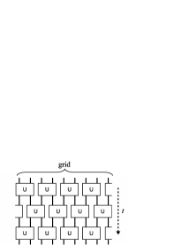
  Figure 1: Structure of a partitioning rule in 1-D.

  This is plainly an invertible CA, since the inverse block map $U^{-1}$ exists and we can apply it to the reverse sequence of partitions.

• The second method of constructing invertible CA rules is the second-order rule approach. This is easiest to understand in the context of a binary CA with cell states 0 and 1 (though it can be generalized to any number of cell states). At any given time $t$, we consider the present state $c^{t}$ of a cell, the states $n_{1}^{t},n_{2}^{t},\ldots$ of its neighbors, and the previous state $c^{t-1}$ of the cell. The rule is determined by choosing an arbitrary binary function $f(c,n_{1},n_{2},\ldots)$ of the cell and its neighbors. The update rule is then

  $$c^{t+1}=c^{t-1}\oplus f(c^{t},n_{2}^{t},n_{1}^{t},\ldots),$$ (1)

  where $\oplus$ represents addition modulo 2.

  This is called a “second-order” rule because the new cell state depends on cell states of two successive times. Any such rule is invertible—indeed, its inverse is the same rule provided the time steps are reversed. That is,

  $$c^{t-1}=c^{t+1}\oplus f(c^{t},n_{2}^{t},n_{1}^{t},\ldots),$$ (2)

  as is easily seen.

• The third way to build an invertible CA is to use use the alternating-subgrid approach. Consider a 2-D square grid of cells, and imagine that the cells are alternately colored black and white in the manner of a checkerboard. (This coloring is a kind of background texture that exists independently of the cell states.) The neighborhood of a cell contains only itself and the cells immediately adjacent to it. Thus, the neighborhood of a black cells consists of itself and four white neighbors, and vice versa.

  The trick is now to update black and white cells in alternate time steps. If $t$ is even only the black cells are updated, and if $t$ is odd only the white cells are updated. Thus, no cell is updated in the same step as its neighbors. If the cell updates according to

  $$c^{t+1}=U(c^{t},n^{t},e^{t},s^{t},w^{t})$$ (3)

  we know that the the states $(n,e,s,w)$ of the four neighbors (north, east, south, west) are not updated at the same time.

  This by itself is not enough to guarantee invertiblity. To do this, we need to require that, for any neighbor configuration $(n,e,s,w)$, the function $U$ is 1-1 and onto on the set of states $c$. Since the states are drawn from a finite set, it suffices to require that $c_{1}\neq c_{2}$ implies

  $$U(c_{1},n,e,s,w)\neq U(c_{2},n,e,s,w)$$ (4)

  for any given choice of $(n,e,s,w)$. Given this condition, there is another function $U^{\prime}$ of the neighborhood that reverses the action of $U$ on each updating cell. The inverse of the alternating-subgrid CA is just another alternating-subgrid CA using $U^{\prime}$ instead of $U$.

The problem of constructing invertible CA rules is the problem of conserving information. The value of the cell state $c^{t}$ at time $t$ constitutes information, and it must always be possible to recover this information from the state of the grid at the next time $t+1$. This might be very complicated. The subsequent state $c^{t+1}$ of the same cell generally depends on the states of several cells (the whole neighborhood) at time $t$, so it is usually not possible to reconstruct $c^{t}$ from $c^{t+1}$ alone. The information about $c^{t}$ is held jointly by many cells at the later time. But all of those cells have meanwhile been influenced by many other cells. To construct an invertible rule, we must somehow devise this local network of information exchange to globally preserve all of the cell state information over time.

The alternating-subgrid technique described above addresses this challenge in a very simple way. At any given step, no cell is both updating its own state and influencing the states of its neighbors. That is, the cell is either listening to its neighbors (and updating its state accordingly) or talking to its neighbors (and influencing their states), but never both. Since the neighbors that influence a cell’s new state retain their own states (for that time step), they retain the necessary “context” information to reverse the cell update operation. See Figure 2.

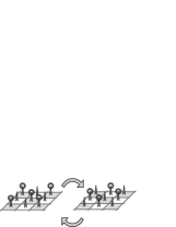
Figure 2: In an alternating-subgrid CA, cells are either transmitting information about their own state or receiving information from transmitting neighbors.

Our approach is to generalize this basic idea, taking what we may call a transmitting-state appraoch. At any given time $t$, each particular cell may be in a “transmitting” or “non-transmitting” state. There may be several distinct states of each type. The update rule for a transmitting state does not depend at all on the cell’s neighbors. The update rule for a non-transmitting state only depends on the cell’s own value and that of its transmitting neighbors. That is, cells in transmitting states are not subject to outside influences, and those that are not transmitting are only influenced by transmitting neighbors.

In the sections that follow, we make this intuitive idea rigorous and show how to use it to create an invertible cellular automaton rule. We briefly explore an example of a 3-state/1-D invertible rule of this type, and show that this rule conserves an additive “energy” quantity on the grid. (Such conservative rules are useful for exploring thermodynamics in discrete systems.) Finally, we add some remarks and pose some unresolved questions.

2 Transmitting and non-transmitting states

Our cellular automata will exist on a regular grid in any number of dimensions. Each cell has a finite set $S$ of states, and its neighborhood consists of itself and $N$ neighboring cells. The update rule is a function of the form $U(c,s_{1},\ldots,s_{N})$, where $c$ is the cell state and $s_{k}$ is the state of the $kth$ neighbor cell. That is,

$$c^{t+1}=U(c^{t},\ldots,s_{k}^{t},\ldots).$$ (5)

Now we identify a subset $T\subseteq S$ of “transmitting” states; non-transmitting states are those not in $T$. There is also a subset $T^{+}\subseteq S$ of the same size as $T$, which we call “post-transmitting” states. We now require five things about the update rule $U$.

1. $c\in T$ iff $U(c,\ldots)\in T^{+}$ for any configuration of neighbor states. Transmitting states, and only those, evolve into post-transmitting states.

2. If $c\in T$ then for any two neighbor states $s_{k},s_{k}^{\prime}\in S$, $U(c,\ldots,s_{k},\ldots)=U(c,\ldots,s_{k}^{\prime},\ldots)$. In other words, if $c$ is a transmitting state, the new cell state does not depend on the particular neighbor states.

3. If $c,c^{\prime}\in T$ and $c\neq c^{\prime}$, then $U(c,\ldots)\neq U(c^{\prime},\ldots)$. Two distinct transmitting states evolve into two distinct post-transmitting states. The update rule on transmitting states (which is effectively a simple map from $T$ to $T^{+}$) is 1-1 (and thus onto).

4. If $c\notin T$, then for any $s_{k},s_{k}^{\prime}\notin T$ we have $U(c,\ldots,s_{k},\ldots)=U(c,\ldots,s_{k}^{\prime},\ldots)$. The values of non-transmitting neighbor states do not affect the update of a non-transmitting cell state.

5. If $c,c^{\prime}\notin T$ and $c\neq c^{\prime}$, then for a given configuration of neighbor states, $U(c,\ldots)\neq U(c^{\prime},\ldots)$. (And from the previous requirement, we know that only the transmitting states in the neighborhood configuration make any difference.)

Our basic claim is that any such rule is reversible. We prove this by explicitly constructing an inverse CA rule $U^{\prime}$ from the forward rule $U$. The inverse rule $U^{\prime}$ has the same neighborhood configuration as $U$. We define the inverse rule as follows.

First, suppose $c^{\prime}\in T^{+}$. Then by conditions 1–3 above, there exists a unique $c\in T$ such that $c^{\prime}=U(c,\ldots)$. For any neighbor configuration, define $U^{\prime}(c^{\prime},\ldots)=c$.

Now suppose $c^{\prime}\notin T^{+}$. Each of the neighbor states $s_{k}^{\prime}$ is either in $T^{+}$ or not. If not, choose $s_{k}$ for that cell to be any state not in $T$ (since its exact value, by condition 4, will not matter). If $s_{k}^{\prime}\in T^{+}$, then choose $s_{k}\in T$ to be the state that maps to $s_{k}^{\prime}$ under $U$ (and thus that $s_{k}^{\prime}$ maps to $s_{k}$ under $U^{\prime}$ as already defined). This means that we can reconstruct the “context” of transmitting neighbor states $s_{k}$ which governed the update of the central cell under $U$. By condition 5, there is a unique $c\in T$ such that

$$c^{\prime}=U(c,\ldots,s_{k},\ldots).$$ (6)

Define $U^{\prime}(c^{\prime},\ldots,s_{k}^{\prime},\ldots)=c$.

We have thus defined the rule $U^{\prime}$ so that it exactly inverts the action of update rule $U$, both for cells that have states in $T$ at time $t$ (that is, $T^{+}$ at time $t+1$) and cells that do not. The CA rule $U$ is therefore invertible.

In an alternating-grid rule, there is a fixed alternating pattern of transmitting and non-transmitting cells, the checkerboard “texture” of black and white cells. In a transmitting-state rule, the pattern of transmitting states is itself dynamically determined by the action of the CA rule $U$. This allows a far greater range of possible rules and behaviors.

3 An example

So far, we have given general conditions for transmitting-state rules without a recipe for creating them. Now we give one such recipe, though the transmitting-state class includes many other kinds of examples. We take the set of cell states to be $S=\{0,1,\ldots,n\}$, containing $n+1$ elements. The set $T$ of transmitting states contains the $n-1$ elements $\{1,\ldots,n-1\}$, and $T^{+}=\{2,\ldots,n\}$. The non-transmitting states only include states 0 and $n$.

The update rule for a transmitting state simply increments the state by 1. That is, for $c\in T$, $U(c,\ldots)=c+1$. The transmitting states thus advance regularly via $1\rightarrow\ldots\rightarrow n-1\rightarrow n$. This automatically satisfies conditions 1–3 for a transmitting-state rule.

How is a cell in a non-transmitting state updated? Non-transmitting states 0 or $n$ can result in non-post-transmitting states 0 or 1. For $c=0$, we choose $U(0,\ldots)$ to be any $\{0,1\}$-valued function of the transmitting states and their arrangement in the neighborhood. (Since the $U$ value depends only on the neighbor states that are in $T$, it satisfies condition 4 above.) We then require $U(n,\ldots)=\overline{U(0,\ldots)}$, the binary complement of the value for the same arrangements of neighborhood transmitting states. This guarantees that we will also satisfy condition 5, yielding a transmitting-state invertible CA rule.

As a specific example, consider a rule on a 1-D grid with a 3-cell neighborhood, so the update rule is of the form $U(l,c,r)$, a function of the left, center and right cells of the neighborhood. The set of states $S=\{0,1,2\}$. The only transmitting state is 1 and the only post-transmitting state is 2. Our update rule is given by

$$l1r \longrightarrow 2\mbox{ for any $l,r$}$$

$$l0r \longrightarrow \left\{\begin{array}[]{cl}1&\mbox{$l=1$ or $r=1$ but not both}\\ 0&\mbox{otherwise}\end{array}\right.$$

$$l2r \longrightarrow \left\{\begin{array}[]{cl}0&\mbox{$l=1$ or $r=1$ but not both}\\ 1&\mbox{otherwise}\end{array}\right.$$

This rule happens to be the 3-state invertible CA numbered 1123289366095 in Wolfram’s enumeration of such rules (as shown in [2], p. 436).

The evolution of a random initial grid under this CA rule is shown in Figure 3.

Figure 3: Spacetime diagram of the behavior of a simple transmitting-state CA in 1-D. Black and white cells are in non-transmitting states, while gray cells represent transmitting states.

As can be seen, this CA rule allows the existence of both persistent spatial structures and long-range information exchange.

The inverse rule for this example is easily found. We can write it this way:

$$l2r \longrightarrow 1\mbox{ for any $l,r$}$$

$$l0r \longrightarrow \left\{\begin{array}[]{cl}1&\mbox{$l=2$ or $r=2$ but not both}\\ 0&\mbox{otherwise}\end{array}\right.$$

$$l1r \longrightarrow \left\{\begin{array}[]{cl}0&\mbox{$l=2$ or $r=2$ but not both}\\ 1&\mbox{otherwise}\end{array}\right.$$

In fact, this is exactly the same rule, with the roles of state 1 and state 2 exchanged.

4 A conserved “energy”

Many invertible CA rules, especially those of interest for modeling physical systems, have a conserved quantity, which we may conveniently call “energy”. The energy is an additive local function. That is, for each small neighborhood $n$ (not necessarily identical to a neighborhood for the CA rule) there is a local energy $\varepsilon_{n}$, and the total energy is just the sum of the local energies of all the overlapping neighborhoods in the grid.

The 3-state rule we describe above turns out to have a straightforward conserved energy. The local energy $\varepsilon$ depends on the joint state of a pair adjacent cells:

$$\begin{array}[]{r}\varepsilon(0,0)=\varepsilon(1,2)=\varepsilon(2,1)=0\\ \varepsilon(0,1)=\varepsilon(1,0)=\varepsilon(0,2)=\varepsilon(2,0)=1\\ \varepsilon(1,1)=\varepsilon(2,2)=2\end{array}$$ (11)

The local energy $\varepsilon$ resides in the “bond” between adjacent cells. The total energy $E$ is the sum of all the bond energies.

Energy $E$ will be conserved provided there exists a local “energy flow” function $f$, which is defined at each cell and depends on the states of that cell and its neighbors. The left-right symmetry of both the update rule and the local energy function means that $f$ needs to be an antisymmetric function. That is, given cell states $l$, $c$ and $r$ at time $t$ (determining the cell state $c^{\prime}$ at time $t+1$), the flow $f$ satisfies

$$f(l,c,r)=-f(r,c,l).$$ (12)

The flow $f$ is to be interpreted as the rightward flow of energy, so that a negative value of $f$ is a flow in the opposite direction.

Just as $\varepsilon$ is localized between cells, we can regard $f$ to be localized between time steps $t$ and $t+1$.

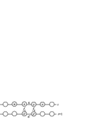
Figure 4: Local energy $\varepsilon$ and energy flow $f$ in a small section of a spacetime diagram for our example CA rule.

Consider then the situation shown in Figure 4. At time $t$, the pair of cells with states $x$ and $y$ have a local bond energy $\varepsilon=\varepsilon(x,y)$. These cell states update to $x^{\prime}$ and $y^{\prime}$ at $t+1$, yielding a new bond energy $\varepsilon^{\prime}=\varepsilon(x^{\prime},y^{\prime})$. (The updated cell states also depend on the adjacent states $w$ and $z$ at time $t$.)

The two cells are associated with energy flows $f_{L}=f(w,x,y)$ and $f_{R}=f(x,y,z)$, also shown in Figure 4. Energy is conserved provided we can show that the change $\Delta\varepsilon$ in local energy is entirely due to the net inward flow $f$ into that region during the cell update—that is, $\varepsilon^{\prime}-\varepsilon=f_{L}-f_{R}$. We must show that, for all cell states $w$, $x$, $y$ and $z$, with $x^{\prime}$ and $y^{\prime}$ given by the CA update rule,

$$\varepsilon(x^{\prime},y^{\prime})-\varepsilon(x,y)=f(w,x,y)-f(x,y,z).$$ (13)

A suitable definition of $f$ for our example can be given as follows: $f(l,c,r)=0$ for any set of states with $l=r$ (a symmetric neighborhood state). Also $f(l,c,r)=0$ for all other states, with the following exceptions:

$$\begin{array}[]{ll}f(0,0,1)=-1&f(1,0,0)=+1\\ f(1,2,0)=-1&f(0,2,1)=+1\\ f(2,0,1)=-1&f(1,0,2)=+1\\ f(1,2,2)=-1&f(2,2,1)=+1\end{array}$$ (14)

We can now in principle check all $3^{4}=81$ possible cases for Equation 13. In practice, we only need to examine a much smaller number of distinct, non-trivial cases. For instance, suppose $(w,x,y,z)=(1,1,2,2)$, so that $(x^{\prime},y^{\prime})=(2,0)$ according to our rule. The initial and final energies are $\varepsilon=\varepsilon(1,2)=0$, while $\varepsilon^{\prime}=\varepsilon(2,0)=1$. The two flows are $f_{L}=f(1,1,2)=0$ and $f_{R}=f(1,2,2)=-1$. Equation 13 clearly holds; and by symmetry it also holds for the reflected case $(w,x,y,z)=(2,2,1,1)$.

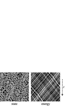
Figure 5: The state evolution of our example CA (left), together with the local energy $\varepsilon$ (right) for the same initial grid.

Figure 5 shows both the state evolution and the distribution of energy for the same initial grid. Energy flows are easily visible as leftward and rightward movements of elementary energy units.

5 Remarks and questions

Transmitting-state cellular automata are a generalization of the alternating-subgrid CA’s, and like them can be used to construct invertible CA rules that produce complex behavior. We have given a general definition of transmitting-state rules and explored a specific example in some detail. Many questions remain.

The alternating-subgrid class includes rules of special interest for modeling physical systems. Consider, for example, the 2-D “reversible Ising” CA rule. In this rule, spins (with $s=\pm 1$) are located on a checkerboard grid and given an Ising-type energy function

$$E=-\sum s_{i}s_{j},$$ (15)

where the sum ranges over all pairs of immediate neighbors $(i,j)$. At any even time $t$, each spin on a white square is inverted provided this does not change the energy; at any odd time $t$ the same procedure is followed for the spins on black squares. The rule is obviously invertible and conserves the Ising energy. Thus it is an interesting model of the microscopic dynamics of a ferromagnetic system. Does the larger transmitting-state class of CA rules, which in effect have shifting, dynamically produced “alternating subgrids”, include other models for more disordered magnetic systems—e.g., for spin glasses?

We also note that our very simple example of a transmitting-state rule (one of the simplest non-trivial rules possible) has a simple conserved energy function. Are such functions more common and/or easier to identify in transmitting-state rules?

Reversible cellular automata have been generalized to quantum cellular automata [6]. Any reversible state function $\mathcal{S}\rightarrow f(\mathcal{S})$ can be made into a unitary map by applying it to a basis of states: $\left|\mathcal{S}\right\rangle\rightarrow U\left|\mathcal{S}\right\rangle=\left|f(\mathcal{S})\right\rangle$. We can always do this for the global state of a CA grid. However, locality of the reversible classical rule does not guarantee locality of the corresponding quantum rule. (This objection does not arise for the partitioning type of reversible CA, so these can always be generalized to a quantum version.) The transmitting-state idea is based on the notion of one-way information flow, and we know that this is impossible in unitary quantum interactions [7]. How does this lead to a failure of locality in the “unitarized” version? Or are there examples that can be made into unitary QCA’s, despite this difficulty?

We would like to express their gratitude for many helpful conversations with Charles Bennett and Tommaso Toffoli. We also acknowledge the support of the Foundational Questions Institute (FQXi), via grant FQXi-RFP-1517.

References

- [1] N. Margolus, Physics and Computation, MIT Ph.D. thesis (1988).
- [2] S. Wolfram, A New Kind of Science, Wolfram Media, Champaign, IL (2002).
- [3] T. Toffoli and N. Margolus, “Invertible cellular automata: A review”, Physica D 45 (1990), 229-253.
- [4] D. Richardson, “Tessellation with local transformations”, J. Comp. Syst. Sci. 6 (1972), 373-388.
- [5] S. Capobianco and T. Toffoli, “Can anything from Noether’s theorem be salvaged for discrete dynamical systems?”, in Calude et al. (eds.), Proceedings of the Unconventional Computation 2011 conference, Lecture Notes in Computer Science 6714, 77-88 (2011). C. H. Bennett, N. Margolus and T. Toffoli, “Bond-energy variables for Ising spin-glass dynamics”, Physical Review B 37 (1988), 2254.
- [6] B. Schumacher and R. Werner, “Reversible quantum cellular automata”, quant-ph/0405174.
- [7] B. Schumacher and M. D. Westmoreland, “Locality and information transfer in quantum operations,” Quantum Information Processing 4, 13 (2004).