How strange is pion electroproduction?

Abstract

We consider pion production in parity-violating electron scattering (PVES) in the presence of nucleon strangeness in the framework of partial wave analysis with unitarity. Using the experimental bounds on the strange form factors obtained in elastic PVES, we study the sensitivity of the parity-violating asymmetry to strange nucleon form factors. For forward kinematics and electron energies above 1 GeV, we observe that this sensitivity may reach about 20% in the threshold region. With parity-violating asymmetries being as large as tens p.p.m., this study suggests that threshold pion production in PVES can be used as a promising way to better constrain strangeness contributions. Using this model for the neutral current pion production, we update the estimate for the dispersive $\gamma Z$-box correction to the weak charge of the proton. In the kinematics of the Qweak experiment, our new prediction reads Re$\,\Box_{\gamma Z}^{V}(E=1.165\,{\rm GeV})=(5.58\pm 1.41)\times 10^{-3}$, an improvement over the previous uncertainty estimate of $\pm 2.0\times 10^{-3}$. Our new prediction in the kinematics of the upcoming MESA/P2 experiment reads Re$\,\Box_{\gamma Z}^{V}(E=0.155\,{\rm GeV})=(1.1\pm 0.2)\times 10^{-3}$.

I Introduction

The discovery of weak neutral current interactions in parity-violating electron scattering (PVES) Prescott:1978tm ; Prescott:1979dh and in atomic parity violation (APV) Wood:1997zq provided an important proof for the structure of the Standard Model (SM). The accuracy of modern experiments provides access to physics beyond the Standard Model (BSM) in a mass range which is comparable or complementary to searches at colliders and in astrophysics Erler:2004in ; Erler:2013xha . Two experiments designed to test the SM running of the weak mixing angle at low energies, Qweak at the Jefferson Laboratory in the U.S. Androic:2013rhu and P2@MESA at Mainz University, Germany Becker:2014hta will constrain SM extensions with mass scales in the 30 - 50 TeV range.

The interpretation of these high-precision experiments in terms of the fundamental SM parameters is based on a similarly precise calculation of electroweak radiative corrections Marciano:1983ss ; Erler:2004in . At the one-loop level, $\gamma Z$-box graph corrections constitute a numerically important contribution. Their evaluation requires knowledge of the hadron structure at low energies, i.e. in a region where perturbation theory can not be applied. Recently, the vector part of these corrections was re-evaluated in the framework of forward dispersion relations Gorchtein:2008px , and its value and uncertainty was found to be considerably larger than previously anticipated. Subsequent work allowed to constrain its central value Gorchtein:2008px ; Sibirtsev:2010zg ; Rislow:2010vi ; Gorchtein:2011mz ; Hall:2013hta , but the size of its uncertainty is still an open question. For the kinematics of the Qweak and P2 experiments, the dispersion representation of the $\gamma Z$-box graph correction involves the inclusive inelastic interference structure functions $F_{1,2}^{\gamma Z}$ integrated over the full kinematical range with a strong emphasis on the low-energy range, $Q^{2}\leq 1$ GeV² and $W\leq 4$ GeV ($Q^{2}$ is the virtuality of the space-like photon or $Z$-boson originating from electron scattering, and $W$ the invariant mass of the hadronic final state $X$ resulting from the process $\gamma^{*}+N\to X$ with $X=\pi N,\,2\pi N$, etc.).

The approach of Refs. Gorchtein:2008px ; Sibirtsev:2010zg ; Rislow:2010vi ; Gorchtein:2011mz ; Hall:2013hta , in the absence of any detailed interference data in the required kinematical range, was based on a purely phenomenological fit to the electromagnetic inelastic total cross section data Christy:2007ve , complemented with an isospin-rotation to predict $F_{1,2}^{\gamma Z}$. Unfortunately, this procedure is essentially ad hoc, and leads to model-dependent uncertainty estimates, reflected by the spread of the uncertainties given in Refs. Rislow:2010vi ; Gorchtein:2011mz ; Hall:2013hta .

In the present work we try to construct the input to the dispersion relations, starting at threshold for pion production, in a more controlled way. In this range, approximately determined by $M+m_{\pi}\leq W\leq 2$ GeV and $Q^{2}\leq 2$ GeV², one can rely on very detailed experimental data for pion photo- and electroproduction that allow for partial wave analyses as implemented in MAID Drechsel:1998hk ; Drechsel:2007if and SAID SAID . In this approach it is also possible to explicitly take account of constraints due to unitarity and symmetries and include dynamical effects of strong rescattering.

In the literature, the weak pion production amplitudes have been constructed from the electromagnetic ones, and observables have been studied upon neglecting strangeness contributions Mukhopadhyay:1998mn ; Sato:2003rq . The main distinction of the present work is in avoiding this assumption. This leads to a natural uncertainty estimate due to strangeness contributions which, firstly, is driven by experimental data on strange form factors from elastic PVES Armstrong:2012bi , and, secondly, brings this uncertainty estimate in direct correspondence with that of inelastic PVES data. Such data above the pion production threshold and reaching into the $\Delta$-resonance region have been taken by the G0 Collaboration at JLab Androic:2012doa and by the A4 Collaboration at MAMI, Mainz A4resPV . Our formalism can also serve as a basis for extracting the strange form factors from threshold pion production in PVES experiments. The advantage of this method lies in the fact that PV asymmetries are large, in the range of several tens of p.p.m. as opposed to a few p.p.m. for asymmetries in elastic PVES, which were traditionally used to access strangeness contributions.

Another closely related topic concerns hadronic parity violation that leads to induced PV contributions in electromagnetic interactions and may be seen in PVES as well as in parity violation in nuclei Zhu:2000gn ; Haxton:2013aca . In elastic PVES, these contributions manifest themselves in a similar way as effects from the axial-vector coupling of the $Z$ boson at the hadronic side, but can be disentangled from the $Z$-exchange contribution in PV pion electroproduction due to a different $Q^{2}$-dependence. Ref. Chen:2000km used the ”DDH best value” of the PV $\pi NN$ coupling constant $h^{1}_{\pi}$ Desplanques:1979hn , and showed that PV threshold $\pi^{+}$ electroproduction at low energies and forward angles is very sensitive to this coupling. On the other hand, there are indications that the actual value of $h^{1}_{\pi}$ is at least four times smaller Page:1987ak . Having in mind such contributions, we will focus on electron energy range $\sim 1$ GeV and not too forward angles. We postpone the detailed discussion of the interplay of hadronic PV effects with the strangeness to the upcoming work.

The article is organized as follows. In Section II we lay out the formalism and define the kinematics, in Section III we explicitly construct the multipoles with the weak vector current and incorporate strangeness contributions. Section IV deals with the sensitivity of the PV asymmetry in inelastic PVES to strange form factors; in Section V we apply the model for weak pion production developed in the previous sections to the calculation of the dispersion $\gamma Z$-correction to the proton’s weak charge. Section VI contains our concluding remarks.

II Kinematics and definitions

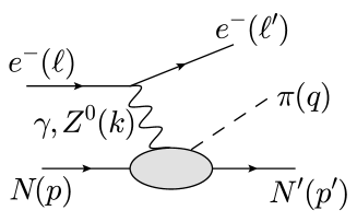
Figure 1: Pion electroproduction via a neutral-current interaction described by the exchange of a virtual photon or a $Z$ boson.

In this work we consider pion electroproduction off a nucleon of mass $M$, $e^{-}(\ell)+N(p)\to e^{-}(\ell^{\prime})+\pi(q)+N^{\prime}(p^{\prime})$, as shown in Fig.  1. The interaction is described by diagrams with the exchange of one boson which carries the four-momentum $k=\ell-\ell^{\prime}$,

$$T = \frac{e^{2}}{Q^{2}}\bar{u}(\ell^{\prime})\gamma^{\mu}u(\ell)\langle N,\pi|J_{\mu}^{EM}|N\rangle$$ (1)

for the contribution of the electromagnetic interaction, and

$$T = -\frac{G_{F}}{2\sqrt{2}}\bar{u}(\ell^{\prime})\gamma^{\mu}(g_{V}^{e}+g_{A}^{e}\gamma_{5})u(\ell)\langle N,\pi|J_{\mu}^{NC}-J_{\mu 5}^{NC}|N\rangle$$ (2)

for the weak neutral current (NC) interaction. We have defined $Q^{2}=-k_{\mu}k^{\mu}>0$. The kinematics of the reaction $\left(\gamma/Z\right)(k)+N(p)\to\pi(q)+N^{\prime}(p^{\prime})$ in the $\pi N$ center of mass frame is completely fixed in terms of three Lorentz scalars for which we take the invariant mass of the hadronic final state $W$, $W^{2}=(p^{\prime}+q)^{2}=(p+k)^{2}$, the virtuality $Q^{2}$ of the initial boson, and the four-momentum transfer to the nucleon $t=(p^{\prime}-p)^{2}<0$. In the following, we will use the center-of-mass frame of the initial nucleon-photon pair (or, equivalently, of the final nucleon-pion pair) defined by $\vec{k}+\vec{p}=\vec{q}+\vec{p}^{\,\prime}=0$. In this reference frame, the kinematics can be specified by the energy of the photon, $\omega$, its virtuality $Q^{2}$, and the pion scattering angle $\theta$. We parametrize the momentum 4-vectors by

$$k^{\mu} = (k^{0},0,0,k)\,,\quad p^{\mu}=(E_{1},0,0,-k)\,,$$

$$q^{\mu} = (E_{\pi},q\sin\theta,0,q\cos\theta)\,,\quad p^{\,\prime\mu}=(E_{2},-\vec{q}\,)\,.$$ (3)

with

$$k^{0} = \frac{W^{2}-M^{2}-Q^{2}}{2W}\,,\quad E_{1}=\frac{W^{2}+M^{2}+Q^{2}}{2W}\,,$$

$$E_{\pi} = \frac{W^{2}-M^{2}+m_{\pi}^{2}}{2W}\,,\quad E_{2}=\frac{W^{2}+M^{2}-m_{\pi}^{2}}{2W}\,,$$

$$|\vec{k}| \equiv k=\frac{\sqrt{[(W-M)^{2}+Q^{2}][(W+M)^{2}+Q^{2}]}}{2W}\,,$$

$$|\vec{q}| \equiv q=\frac{\sqrt{[W^{2}-(M+m_{\pi})^{2}][W^{2}-(M-m_{\pi})^{2}]}}{2W}\,,$$

$$\cos\theta = \frac{2k^{0}E_{\pi}+t+Q^{2}-m_{\pi}^{2}}{2kq}\,.$$ (4)

II.1 Invariant amplitudes

The invariant amplitudes with the vector current were introduced, e.g., in Ref. Adler:1968tw as

$$\langle N,\pi|J_{\mu}^{EM,\,NC}|N\rangle = \sum_{i=1}^{6}V^{\gamma,Z}_{i}(W^{2},Q^{2},t)\bar{U}_{f}O^{\mu}_{V_{i}}U_{i}\,,$$ (5)

with

$$O^{\mu}_{V_{1}} = \frac{i}{2}\left(\gamma^{\mu}\not\!k\,-\not\!k\,\gamma^{\mu}\right)\gamma_{5}\,,$$

$$O^{\mu}_{V_{2}} = -2i\left(P^{\mu}(q\cdot k)-q^{\mu}(P\cdot k)\right)\gamma_{5}\,,$$

$$O^{\mu}_{V_{3}} = \left(\gamma^{\mu}(q\cdot k)-q^{\mu}\not\!k\right)\gamma_{5}\,,$$

$$O^{\mu}_{V_{4}} = 2\left(\gamma^{\mu}(P\cdot k)-P^{\mu}\not\!k\right)\gamma_{5}-2MO^{\mu}_{V_{1}}\,,$$

$$O^{\mu}_{V_{5}} = -i\left(k^{\mu}(q\cdot k)-q^{\mu}k^{2}\right)\gamma_{5}\,,$$

$$O^{\mu}_{V_{6}} = \left(k^{\mu}\not\!k-\gamma^{\mu}k^{2}\right)\gamma_{5}\,,$$ (6)

where $U_{i}\,(U_{f})$ stand for the initial (final) nucleon Dirac spinor, and we have used the average nucleon four-momentum $P=(p+p^{\prime})/2$. Similarly, the axial-vector part is separated as

$$\langle N,\pi|J_{\mu 5}^{NC}|N\rangle = \sum_{i=1}^{8}A^{Z}_{i}(W^{2},Q^{2},t)\bar{U}_{f}O^{\mu}_{A_{i}}U_{i}\,,$$ (7)

with

$$O^{\mu}_{A_{1}} = -\frac{i}{2}\left(\gamma^{\mu}\not\!q\,-\not\!q\,\gamma^{\mu}\right)\,,$$

$$O^{\mu}_{A_{2}} = 2iP^{\mu}\,,$$

$$O^{\mu}_{A_{3}} = iq^{\mu}\,,$$

$$O^{\mu}_{A_{4}} = -M\gamma^{\mu}\,,$$

$$O^{\mu}_{A_{5}} = 2P^{\mu}\not\!k\,,$$

$$O^{\mu}_{A_{6}} = q^{\mu}\not\!k\,,$$

$$O^{\mu}_{A_{7}} = ik^{\mu}\,,$$

$$O^{\mu}_{A_{8}} = k^{\mu}\not\!k\,.$$ (8)

The scalar amplitudes $V_{i}^{\gamma,Z}$, $A_{i}^{Z}$ are functions of the invariants $W^{2}$, $Q^{2}$ and $t$. The last two structures $O^{\mu}_{A_{7,8}}$ are lepton mass terms and do not contribute to the neutral current process studied here.

II.2 Multipole decomposition

It is common to evaluate the covariant tensors introduced in the previous subsection in the center-of-mass frame of the pion and the final nucleon, relating the invariant amplitudes to the CGLN amplitudes CGLN

$$\epsilon_{\mu}\sum_{j=1}^{6}V^{\gamma,Z}_{j}(W^{2},Q^{2},t)\bar{U}_{f}O^{\mu}_{V_{j}}U_{i} = \sum_{j=1}^{6}{\cal{F}}_{j}\chi^{\dagger}_{f}\Sigma_{j}\chi_{i},$$

$$\epsilon_{\mu}\sum_{j=1}^{6}A^{Z}_{j}(W^{2},Q^{2},t)\bar{U}_{f}O^{\mu}_{A_{j}}U_{i} = \sum_{j=1}^{6}{\cal{G}}_{j}\chi^{\dagger}_{f}\tilde{\Sigma}_{j}\chi_{i},$$ (9)

with $\epsilon_{\mu}$ the photon or $Z$ polarization vector, ${\cal{F}}_{j},{\cal{G}}_{j}$ scalar amplitudes, $\chi_{i}(\chi_{f})$ the Weyl spinors for initial (final) nucleon, respectively, and $\Sigma_{j},\tilde{\Sigma}_{j}$ matrices in the spinor space. The CGLN amplitudes allow for a decomposition into multipoles,

$${\cal{F}}_{j} = \sum_{l}\left\{a_{j,l\pm}E_{l\pm}+b_{j,l\pm}M_{l\pm}+c_{j,l\pm}S_{l\pm}\right\},$$

$${\cal{G}}_{j} = \sum_{l}\left\{\tilde{a}_{j,l\pm}{\cal{E}}_{l\pm}+\tilde{b}_{j,l\pm}{\cal{M}}_{l\pm}+\tilde{c}_{j,l\pm}{\cal{S}}_{l\pm}\right\}.$$ (10)

Above, $E_{l\pm},M_{l\pm},S_{l\pm}$ are the multipoles describing the vector electric, magnetic and scalar transition to the $\pi N$-state with the angular orbital momentum $l$ and the total orbital momentum $j=l\pm 1/2$, and similarly ${\cal{E}}_{l\pm},{\cal{M}}_{l\pm},{\cal{S}}_{l\pm}$ describe transitions with the axial vector interaction. The multipoles are functions of $W$ and $Q^{2}$ only, and the angular dependence in terms of Legendre polynomials and their derivatives is contained in the coefficients $a,b,c,\tilde{a},\tilde{b},\tilde{c}$. The explicit form of the coefficients of the matrices $a,b,c$ for the vector case can be found in Ref. Berends:1967vi and $\tilde{a},\tilde{b},\tilde{c}$ in Ref. Adler:1968tw for the axial-vector case.

II.3 Isospin structure

Isospin is not conserved by the electromagnetic interaction. The one-photon exchange diagram has, therefore, an isoscalar and an isovector component. Combining $I=0,1$ of the photon and $I=1$ of the pion would lead to three possible isospin amplitudes for $I=0,1,2$. From the $t$-channel perspective, i.e. for pion photoproduction $\gamma\pi\to N\bar{N}$, however, only $I=0$ or $I=1$ are possible. As a result, there are three independent isospin channels which we denote by $M^{0}$ and $M^{\pm}$. The scattering amplitude can thus be separated as

$$M = M^{0}\bar{\chi}_{f}(\vec{\tau}\cdot\vec{\pi})\chi_{i}+M^{+}\bar{\chi}_{f}\frac{1}{2}\{(\vec{\tau}\cdot\vec{\pi}),\tau_{3}\}\chi_{i}+M^{-}\bar{\chi}_{f}\frac{1}{2}[(\vec{\tau}\cdot\vec{\pi}),\tau_{3}]\chi_{i}\,,$$ (11)

with $\chi_{i,f}$ the two-component nucleon’s isospinors, $\vec{\tau}$ the Pauli matrices and $\vec{\pi}$ denote the pion isovectors. In terms of these isospin-channel amplitudes, charge-channel amplitudes are expressed as

$$M^{\pi^{+}n} = \sqrt{2}(M^{0}+M^{-})\,,$$

$$M^{\pi^{-}p} = \sqrt{2}(M^{0}-M^{-})\,,$$

$$M^{\pi^{0}p} = M^{+}+M^{0}\,,$$

$$M^{\pi^{0}n} = M^{+}-M^{0}\,.$$ (12)

These relations are equally valid for multipole, invariant or CGLN amplitudes.

The isospin decomposition of the electromagnetic and weak neutral current in terms of quark currents (we consider the three lightest flavors $u,d,s$ only) reads

$$J_{\mu}^{EM} = \sum_{q}e^{q}\bar{u}_{q}\gamma_{\mu}u_{q}=\bar{q}\gamma_{\mu}\left(\frac{1}{6}\mathbb{1}+\frac{1}{2}\tau_{3}\right)q-\frac{1}{3}\bar{s}\gamma_{\mu}s\,,$$

$$J_{\mu}^{NC} = \sum_{q\in N}g_{V}^{q}\bar{u}_{q}\gamma_{\mu}u_{q}=\bar{q}\gamma_{\mu}\left(\xi_{V}^{I=0}\frac{1}{6}\mathbb{1}+\xi_{V}^{I=1}\frac{1}{2}\tau_{3}\right)q+\xi_{V}^{s}\bar{s}\gamma_{\mu}s\,,$$

$$J_{\mu 5}^{NC} = \sum_{q\in N}g_{A}^{q}\bar{u}_{q}\gamma_{\mu}\gamma_{5}u_{q}=\bar{q}\gamma_{\mu}\gamma_{5}\left(\xi_{A}^{I=0}\frac{1}{6}\mathbb{1}+\xi_{A}^{I=1}\frac{1}{2}\tau_{3}\right)q+\xi_{A}^{s}\bar{s}\gamma_{\mu}\gamma_{5}s\,,$$ (13)

with $q=\left(\begin{array}[]{c}u\\ d\end{array}\right)$. At tree level in the Standard Model and according to the normalization defined in Eq. (2), the coupling constants appearing in these equations are determined by the weak mixing angle, $\sin^{2}\theta_{W}$, and given by $\xi_{V}^{I=1}=2-4\sin^{2}\theta_{W}$, $\xi_{V}^{I=0}=-4\sin^{2}\theta_{W}$, $\xi_{A}^{I=1}=2$, $\xi_{A}^{I=0}=0$, $\xi_{V}^{s}=-1/2+(2/3)\sin^{2}\theta_{W}$, and $\xi_{A}^{s}=-1/2$. From this decomposition we obtain the standard expressions for the weak form factors of the nucleon,

$$G_{E,M}^{Z,\,p} = -G_{E,M}^{\gamma,\,n}+(1-4\sin^{2}\theta_{W})G_{E,M}^{\gamma,\,p}-G_{E,M}^{s}\,,$$

$$G_{E,M}^{Z,\,n} = -G_{E,M}^{\gamma,\,p}+(1-4\sin^{2}\theta_{W})G_{E,M}^{\gamma,\,n}-G_{E,M}^{s}\,.$$ (14)

In the same way, the flavor decomposition of the amplitudes for weak vector pion production, identifying, e.g., $M^{-}=\frac{1}{\sqrt{2}}(M^{\pi^{+}n}-M^{\pi^{-}p})$, and keeping strangeness, can be decomposed as

$$M^{\pi^{+}n}_{Z} = -M^{\pi^{-}p}_{\gamma}+(1-4\sin^{2}\theta_{W})M^{\pi^{+}n}_{\gamma}-\sqrt{2}M_{s}\,,$$

$$M^{\pi^{-}p}_{Z} = -M^{\pi^{+}n}_{\gamma}+(1-4\sin^{2}\theta_{W})M^{\pi^{-}p}_{\gamma}-\sqrt{2}M_{s}\,,$$

$$M^{\pi^{0}p}_{Z} = M^{\pi^{0}n}_{\gamma}+(1-4\sin^{2}\theta_{W})M^{\pi^{0}p}_{\gamma}-M_{s}\,,$$

$$M^{\pi^{0}n}_{Z} = M^{\pi^{0}p}_{\gamma}+(1-4\sin^{2}\theta_{W})M^{\pi^{0}n}_{\gamma}+M_{s}\,.$$ (15)

The presence of the strangeness contribution is the main distinction of this analysis from other calculations of pion production in electroweak reactions.

III Vector multipoles from isospin symmetry and strangeness form factors

Upon neglecting the strangeness contribution, the vector multipoles in weak NC pion-production is given exactly in terms of the electromagnetic multipoles given in Eq. (15). To our knowledge, this is how pion production is dealt with in all phenomenological models that relate pion production in electromagnetic and weak NC reactions. The aim of this section is to go beyond this approximation and model the strangeness contributions.

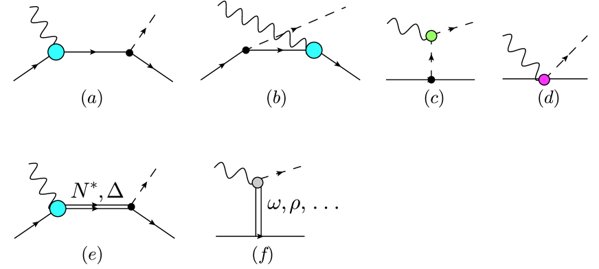
Figure 2: Isobar model for pion-production. (a) -(d) are Born contributions, (e) are resonance contributions and the $t$-channel vector exchange diagrams are shown in (f). The blobs indicate the elastic nucleon and pion, and various transition form factors.

We start from the isobar model as implemented in MAID Drechsel:1998hk ; Drechsel:2007if . The pion-production amplitude can be represented as a sum of tree-level amplitudes, as shown in Fig. 2. These can be modeled in terms of tree-level coupling constants and form factors. Rescattering effects are incorporated following the unitarization procedure in the $K$-matrix approach used in MAID Drechsel:1998hk . There, the unitarized Born amplitude $M^{B,\alpha}_{\gamma\pi}$ is obtained from the tree-level Born amplitude $B^{\alpha}_{\gamma\pi}$ and the elastic pion-nucleon scattering amplitude $t^{\alpha}_{\pi N}=[\eta_{\alpha}\exp(2i\delta_{\alpha})-1]/2i$ (taken from the SAID analysis Arndt:1995ak ) expressed in terms of phase shifts $\delta_{\alpha}$ and inelasticities $\eta_{\alpha}$ as

$$M^{B,\alpha}_{\gamma\pi}=B^{\alpha}_{\gamma\pi}[1+it^{\alpha}_{\pi N}]\,,$$ (16)

where the index $\alpha=(j$, $l$, $I$,…) carries all relevant quantum numbers: total and orbital angular momentum, isospin, multipolarity etc. The unitarized Born amplitude defined in this way has the phase of the pion-nucleon scattering amplitude below the two-pion production threshold and obeys the Watson theorem. Note that the Born amplitude described by the sum of the graphs (a) - (d) in Fig. 2 is gauge invariant, which is achieved by requiring a certain form of the form factor of the contact term, graph (d) in this figure Berends:1967vi ; Adler:1968tw . Gauge invariance makes such a unitarization procedure for the Born part meaningful. The MAID approach consists then in adding further contributions like vector meson exchange contributions (graph (f)) within the same unitarization procedure, and resonances (graph (e)) with an appropriate phase, such that the full amplitude $M^{\alpha}_{\gamma\pi}=M^{B,\alpha}_{\gamma\pi}+M^{V,\alpha}_{\gamma\pi}+M^{R,\alpha}_{\gamma\pi}$ has the correct phase Drechsel:1998hk .

Since the pion is an isovector, only the isovector components of the photon and $Z$ boson couple to the pion field. The same is true for all $N\to\Delta$ transitions. Correspondingly, only $ZNN$ and $ZNN^{*}$ couplings can obtain additional contributions from strangeness. This statement operates with ”bare” couplings of the photon. However, rescattering effects that could modify the tree level amplitudes are due to the strong interaction which conserves isospin and flavor.

The most straightforward way to estimate the strangeness contribution is to use the available experimental information on strange form factors of the nucleon. A recent global analysis Armstrong:2012bi gives the following values of the strange electric and magnetic form factors of the nucleon at $Q^{2}=0.1$ GeV²,

$$G_{M}^{s}(0.1\,{\rm GeV}^{2}) = 0.29\pm 0.21\,,$$

$$G_{E}^{s}(0.1\,{\rm GeV}^{2}) = -0.008\pm 0.016\,.$$ (17)

For this analysis, the strange form factors were parametrized as $G_{E}^{s}=\rho_{s}\tau G_{D}(Q^{2})$ and $G_{M}^{s}=\mu_{s}G_{D}(Q^{2})$, with $\tau=Q^{2}/(4M^{2})$, $G_{D}(Q^{2})=(1+Q^{2}/\Lambda_{V}^{2})^{-2}$, and $\Lambda_{V}=0.84$ GeV. With this parametrization, extrapolating $G_{M}^{s}$ from $Q^{2}=0.1$ GeV² to the origin one obtains $\mu_{s}=0.38\pm 0.27$. Analyses based on lattice QCD tend to give smaller values of the strange form factors with a much smaller uncertainty Shanahan:2014tja ; Green:2015wqa . For our purpose, the values given in Eq. (17) are sufficient, since one of the goals of this work is to propose a new way of extracting the strangeness contribution from the experimental data. The estimates from lattice QCD are automatically included in the explored parameter range. We also note that the values given above, if rewritten in terms of Dirac and Pauli strange form factors using $G_{M}^{s}=F_{1}^{s}+F_{2}^{s}$ and $G_{E}^{s}=F_{1}^{s}-\tau F_{2}^{s}$, are consistent with $F_{1}^{s}=0$ and $F_{2}=\mu_{s}G_{D}(Q^{2})$.

The strange magnetic moment contribution to the Born multipoles can now be calculated in a straightforward way, and we make use of the expressions for the Born multipoles published in Berends et al. Berends:1967vi . However, we have to extend the analysis of Berends:1967vi where the $\pi NN$ coupling is assumed to be purely pseudoscalar, whereas MAID uses a combination of pseudoscalar and pseudovector couplings,

$$\langle N|\pi^{a}|N\rangle=\frac{g_{\pi NN}}{2M}\bar{N}(p^{\prime})\not\!q\gamma_{5}\tau^{a}N(p)\frac{\Lambda_{m}^{2}}{\Lambda_{m}^{2}+{\vec{q}\,}^{2}}+g_{\pi NN}\bar{N}(p^{\prime})\gamma_{5}\tau^{a}N(p)\frac{\vec{q}\,^{2}}{\Lambda_{m}^{2}+\vec{q}\,^{2}}\,,$$ (18)

with $\vec{q}$ the three-momentum of the pion. The parameter $\Lambda_{m}=450$ MeV describes the transition from a pseudo-vector coupling at the pion production threshold (where $|\vec{q}|=0$) to a pseudo-scalar coupling at high energies. It is this form that we adopt here. As a consequence, an additional contact term appears which contributes to four of the multipoles, nameley to $E_{0+}$, $M_{1-}$, $S_{0+}$, and $S_{1-}$. We present the full expressions for the Born strangeness contributions to the multipoles in Appendix A.

In Figs. 3 - 8 we display results for the first few multipoles according to the procedure described above. In all figures, the dotted curves represent the MAID results for electromagnetic pion production, while the dashed curves include the weak neutral current contributions assuming exact isospin symmetry with no strangeness, and the solid curves correspond to the weak neutral current multipoles including strangeness using the strange magnetic moment $\mu_{s}=0.38$. Thus the difference between the solid and the dashed curves is a measure of the sensitivity of the multipoles to the strange magnetic moment.

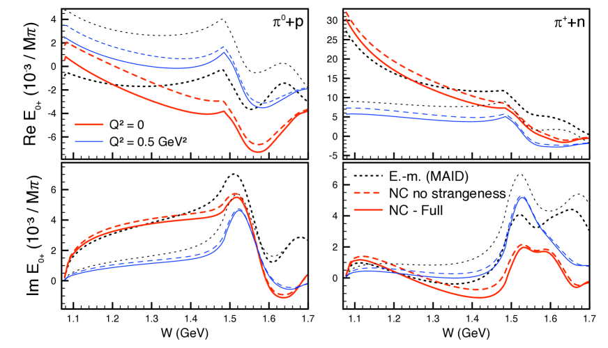
Figure 3: Results for the electromagnetic and weak NC multipole $E_{0+}$ in the charge channels $\gamma(Z)+p\to\pi^{0}+p$ (left panels) and $\gamma(Z)+p\to\pi^{+}+n$ (right panels) in units of ($10^{-3}/m_{\pi}$) as function of $W$ in GeV. The upper panels show the real part, while the lower panels show the imaginary part of the multipole. The thick (thin) curves display results for $Q^{2}=0$ ($Q^{2}=0.5$ GeV²), respectively. The dotted curves correspond to the electromagnetic result from MAID, the dashed curve represent the result for the weak NC multipole neglecting the strangeness contribution, whereas the solid curves show the full weak NC multipole including strangeness.

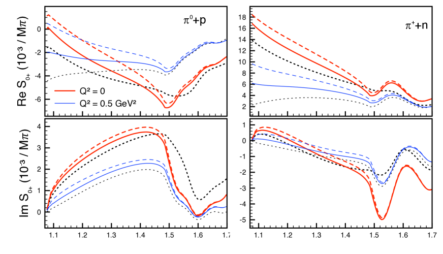
Figure 4: Same as in Fig. 3 for the multipole $S_{0+}$.

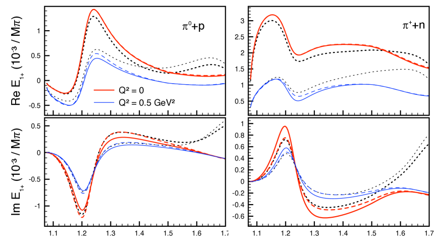
Figure 5: Same as in Fig. 3 for the multipole $E_{1+}$.

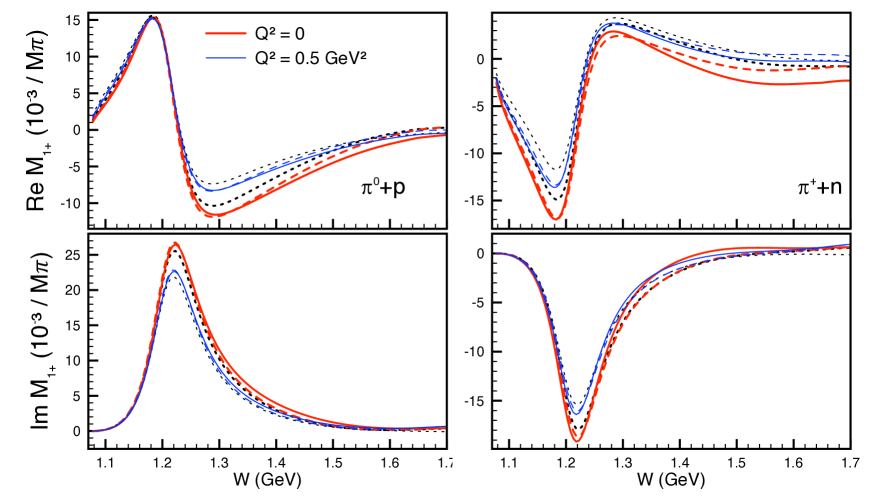
Figure 6: Same as in Fig. 3 for the multipole $M_{1+}$.

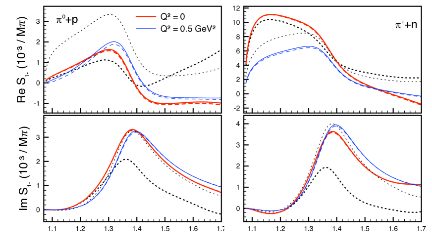
Figure 7: Same as in Fig. 3 for the multipole $S_{1-}$.

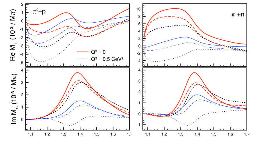
Figure 8: Same as in Fig. 3 for the multipole $M_{1-}$.

IV Sensitivity of the PV asymmetry to $\mu_{s}$ at threshold and in the $\Delta$-region

Weak pion production can be accessed, e.g., in parity-violating electron scattering (PVES). We will consider inclusive scattering here, i.e., we assume that only the electron in the final state is detected. In terms of the electromagnetic and $\gamma Z$ interference cross sections $\sigma_{T,L,A}^{\gamma,\gamma Z}$ the asymmetry for scattering of a beam of longitudinally polarized electrons off unpolarized protons reads

$$A^{PV} = -\frac{G_{F}Q^{2}}{4\sqrt{2}\pi\alpha_{em}}\frac{\sigma_{T}^{\gamma Z}+\epsilon\sigma_{L}^{\gamma Z}+(1-4\sin^{2}\theta_{W})\sqrt{1-\epsilon^{2}}\sigma_{A}^{\gamma Z}}{\sigma_{T}^{\gamma}+\epsilon\sigma_{L}^{\gamma}}\,,$$ (19)

with the usual polarization parameter $\epsilon$ ranging from 0 for backward scattering to 1 for forward scattering,

$$\epsilon=\left[1+2(\nu^{2}+Q^{2})/Q^{2}\tan^{2}(\theta/2)\right]^{-1}\,.$$ (20)

$\nu=E-E^{\prime}$ is the energy of the virtual photon in the laboratory reference frame. The contribution from $\pi N$ final states, ${}^{\pi N}\sigma_{T,L,A}^{\gamma,\gamma Z}$, to these cross sections are expressed in terms of multipoles as

$${}^{\pi N}\sigma_{T}^{\gamma Z} = 4\pi\frac{q}{k_{\gamma}^{CM}}\sum_{l}(l+1)^{2}\left[\frac{l+2}{2}{\rm Re}(E_{l+}^{\gamma\,*}E_{l+}^{Z}+M_{(l+1)-}^{\gamma\,*}M_{(l+1)-}^{Z})\right.$$

$$\qquad\qquad\qquad\qquad\quad\left.+\frac{l}{2}{\rm Re}(M_{l+}^{\gamma\,*}M_{l+}^{Z}+E_{(l+1)-}^{\gamma\,*}E_{(l+1)-}^{Z})\right]\,,$$

$${}^{\pi N}\sigma_{L}^{\gamma Z} = 2\pi\frac{q}{k_{\gamma}^{CM}}\frac{Q^{2}}{\vec{k}\,^{2}}\sum_{l}(l+1)^{3}{\rm Re}(S_{l+}^{\gamma\,*}S_{l+}^{Z}+S_{(l+1)-}^{\gamma\,*}S_{(l+1)-}^{Z})\,,$$

$${}^{\pi N}\sigma_{A}^{\gamma Z} = 4\pi\frac{q}{k_{\gamma}^{CM}}\sum_{l}(l+1)^{2}\left[\frac{l+2}{2}{\rm Re}(E_{l+}^{\gamma\,*}{\cal{M}}_{l+}^{Z}+M_{(l+1)-}^{\gamma\,*}{\cal{E}}_{(l+1)-}^{Z})\right.$$

$$\qquad\qquad\qquad\qquad\quad\left.+\frac{l}{2}{\rm Re}(M_{l+}^{\gamma\,*}{\cal{E}}_{l+}^{Z}+E_{(l+1)-}^{\gamma\,*}{\cal{M}}_{(l+1)-}^{Z})\right]\,,$$

$${}^{\pi N}\sigma_{T}^{\gamma} = 4\pi\frac{q}{k_{\gamma}^{CM}}\sum_{l}(l+1)^{2}\left[\frac{l+2}{2}(|E_{l+}^{\gamma}|^{2}+|M_{(l+1)-}^{\gamma}|^{2})+\frac{l}{2}(|M_{l+}^{\gamma}|^{2}+|E_{(l+1)-}^{\gamma}|^{2})\right]\,,$$

$${}^{\pi N}\sigma_{L}^{\gamma} = 2\pi\frac{q}{k_{\gamma}^{CM}}\frac{Q^{2}}{\vec{k}\,^{2}}\sum_{l}(l+1)^{3}\left[|S_{l+}^{\gamma}|^{2}+|S_{(l+1)-}^{\gamma}|^{2}\right]\,.$$ (21)

Here we have used $k_{\gamma}^{CM}=(W^{2}-M^{2})/2W$ which stands for the real photon three-momentum in the center-of-mass frame. Expressions for ${}^{\pi N}\sigma_{T,L}^{\gamma}$ in terms of multipoles have been obtained, e.g., in Ref. Drechsel:1992pn . In contrast to that reference, here the longitudinal cross section is written in terms of scalar, $S_{l\pm}$, rather than longitudinal multipoles, $L_{l\pm}$. The two sets of multipole moments are related by gauge invariance. Expressions for the interference cross sections ${}^{\pi N}\sigma_{T,L}^{\gamma Z}$ are a straightforward generalization of their electromagnetic counterparts, but to our knowledge have not been reported in the literature before, as is the case with the axial term ${}^{\pi N}\sigma_{A}^{\gamma Z}$. Note that the longitudinal axial-vector multipoles do not enter ${}^{\pi N}\sigma_{A}^{\gamma Z}$ which is hence purely transverse.

As in Ref. Mukhopadhyay:1998mn , the PV asymmetry defined in Eq. (19) can be represented as a sum of three terms,

$$A^{PV} = -\frac{G_{F}Q^{2}}{4\sqrt{2}\pi\alpha_{em}}\left[A_{1}+A_{2}+A_{3}\right]\,.$$ (22)

The first term, $A_{1}=2-4\sin^{2}\theta_{W}$, is model independent and results from isolating the isovector contribution in the numerator and denominator. The other two terms encode the isoscalar and strange ($A_{2}$) and the axial-vector ($A_{3}$) contributions. This form follows from the isospin decomposition of Eq. (15) but we do not explicitly rewrite Eq. (19) here.

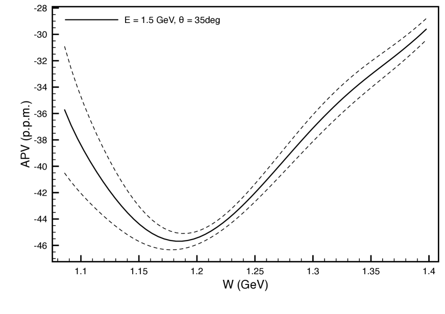
Figure 9: PV asymmetry in the kinematics of A4@MAMI experiment with beam energy $E=1.5$ GeV and fixed electron scattering angle $\theta_{e}=35^{\circ}$. The various curves demonstrate the sensitivity to strange magnetic moment: the solid curve corresponds to the central value $\mu_{s}=0.38$, and the band between the upper and lower dashed curves indicates the uncertainty range $\delta\mu_{s}=\pm 0.27$.

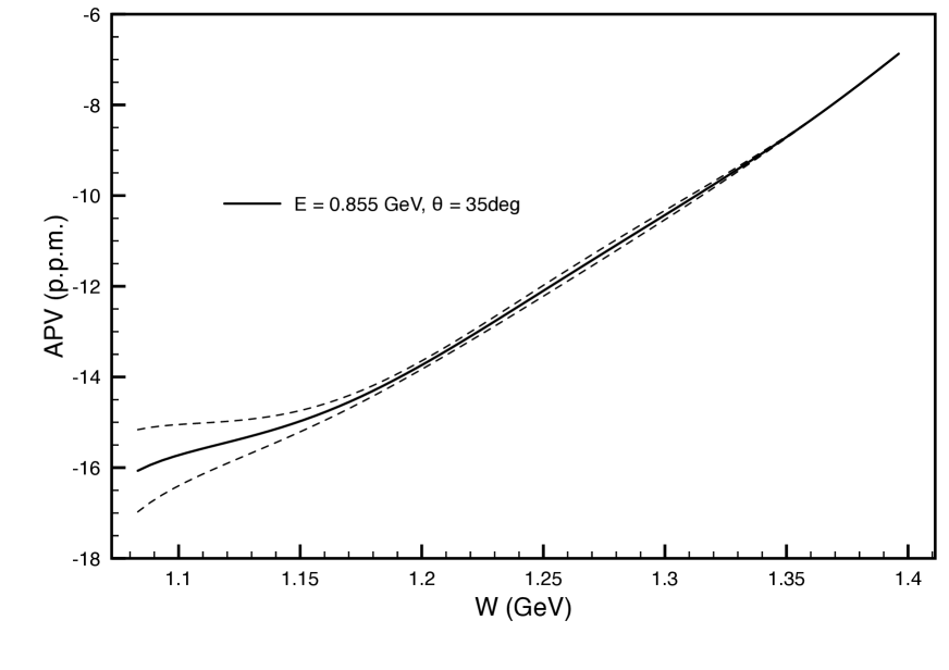
Figure 10: Same as in Fig. 9 for $E=0.855$ GeV.

We are interested in studying the sensitivity of the parity-violating asymmetry to strangeness contributions. To simplify the discussion and to keep the analysis uncontaminated, we start with results without taking the axial multipoles into account. In fact, their contribution is suppressed by the small weak charge of the electron, with $1-4\sin^{2}\theta_{W}(0)\approx 0.048$. In addition, the factor $\sqrt{1-\epsilon^{2}}$ leads to a further suppression for forward kinematics; however, this suppression is not there at backward angles.

In Figs. 9 and 10, we plot our results as a function $W$ in the range between the pion production threshold and the $\Delta$-resonance region assuming forward kinematics as measured in the A4 experiment at MAMI. We see that in this kinematic range there is considerable sensitivity to the strangeness contribution at the level of 10 – 20%, as indicated by the difference between the solid and dashed lines in Figs. 9, 10. This sensitivity is quite promising in view of the high precision of the experimental data which are at the level of 5% A4resPV . A targeted analysis of the available inelastic PVES data between threshold and the $\Delta$ resonance region will offer an alternative way to constrain strangeness form factors of the nucleon, virtually independent of the conventional measurements of elastic PVES.

Historically, the parity-violating asymmetry in electron scattering has been proposed to measure the axial $N\to\Delta$ transition Mukhopadhyay:1998mn . Numerically, its contribution at the $\Delta$ resonance position in the backward kinematics of the G0 experiment is at the level of 6% Androic:2012doa . Our estimates show that at the $\Delta$ position an extraction of the axial $N\to\Delta$ transition would still be possible since the uncertainty due to strangeness is below 3%. The largest sensitivity to strange form factors is, not unexpectedly, observed between the threshold and the $\Delta$ resonance.

V An update of $\gamma Z$-box graph corrections to elastic PVES experiments

The $\gamma Z$-box graph corrections to elastic PVES have attracted significant attention recently. They can be evaluated in an approach based on dispersion relations from $\gamma Z$ interference structure functions for inelastic $ep$ scattering. Their vector part, ${\rm Re}\,\Box^{V}_{\gamma Z}$, is sensitive to low-energy form factor input and depends strongly on the beam energy. For the kinematics of the Qweak experiment the box graph corrections exceed the previously claimed theory uncertainty by a factor of 8. Currently, the size of ${\rm Re}\,\Box^{V}_{\gamma Z}$ has settled at $5.4\times 10^{-3}$ Gorchtein:2008px ; Sibirtsev:2010zg ; Rislow:2010vi ; Gorchtein:2011mz ; Hall:2013hta , but the uncertainty estimates range from $0.4\times 10^{-3}$ Hall:2013hta to $2.0\times 10^{-3}$ Gorchtein:2011mz . In the framework of forward dispersion relations, the $\gamma Z$-box correction obeys a sum rule in terms of the inclusive interference structure functions $F_{1,2}^{\gamma Z}$, as function of the lab energy of the electron,

$${\rm Re}\,\Box^{V}_{\gamma Z}(E) = \frac{\alpha_{em}}{2\pi M^{2}E}\int\limits_{(M+m_{\pi})^{2}}^{\infty}dW^{2}\int\limits_{0}^{\infty}\frac{dQ^{2}}{1+Q^{2}/M_{Z}^{2}}\left\{\left[\frac{1}{2E}\ln\left|\frac{E+\omega}{E-\omega}\right|-\frac{1}{\omega}\right]F_{1}^{\gamma Z}(W^{2},Q^{2})\right.$$ (23)

$$\left.+\frac{M}{Q^{2}}\left[\frac{E}{\nu}\left(1-\frac{Q^{2}}{4E^{2}}\right)\ln\left|\frac{E+\omega}{E-\omega}\right|+\ln\left|1-\frac{E^{2}}{\omega^{2}}\right|-\frac{Q^{2}}{M\omega}\right]F_{2}^{\gamma Z}(W^{2},Q^{2})\right\}\,,$$

where $\nu=(W^{2}-M^{2}+Q^{2})/2M$ is the virtual photon energy in the laboratory frame, and $\omega=(\nu+\sqrt{\nu^{2}+Q^{2}})/2$. The integral requires knowledge of the structure functions $F_{1,2}^{\gamma Z}$ in the whole kinematic range in the two variables $W$ and $Q^{2}$. For a meaningful evaluation of this integral, the $\pi N$ contribution to the inclusive structure functions developed in the previous section needs to be extended to $W>2$ GeV and $Q^{2}>2$ GeV², and contributions from higher-mass states need to be included. First, we deal with extending the $\pi N$ state contribution to higher energies using the Regge theory framework. Assuming that at $W=2$ GeV the background contribution (mainly the vector meson exchanges) dominate over the resonances in the cross section, we can use the Regge theory expectation $F_{1}(W\to\infty)\sim(W^{2}/1\,{\rm GeV}^{2})^{\alpha_{M}(0)}$ and $F_{2}(W\to\infty)\sim(W^{2}/W_{0}^{2})^{\alpha_{M}(0)-1}$. The meson Regge trajectory $\alpha_{M}(t)=\alpha_{M}^{0}+\alpha^{\prime}_{M}t$ is taken at $t=0$, and the relevant $\rho$-$\omega$ trajectories correspond to $\alpha_{\rho}^{0}\approx\alpha_{\omega}^{0}\approx 0.5$. Correspondingly, the simple Ansatz

$$F_{1}^{\pi N}(W\geq 2\,{\rm GeV},Q^{2}) = F_{1}^{\pi N}(2\,{\rm GeV},Q^{2})\times\left(\frac{W}{2\,{\rm GeV}}\right)\,,$$

$$F_{2}^{\pi N}(W\geq 2\,{\rm GeV},Q^{2}) = F_{2}^{\pi N}(2\,{\rm GeV},Q^{2})\times\left(\frac{2\,{\rm GeV}}{W}\right)$$ (24)

was adopted. The $Q^{2}$-dependence beyond $Q^{2}=2$ GeV² is assumed to follow a dipole $\sim[1+Q^{2}/\Lambda_{V}^{2}]^{-2}$ with $\Lambda_{V}=0.84$ GeV², reminiscent of nucleon form factors,

$$F_{1,2}^{\pi N}(W,Q^{2}\geq 2\,{\rm GeV}^{2}) = F_{1,2}^{\pi N}(W,2\,{\rm GeV}^{2})\times\left(\frac{\Lambda_{V}^{2}+2\,{\rm GeV}^{2}}{\Lambda_{V}^{2}+Q^{2}}\right)^{2}\,.$$ (25)

This model is not very sophisticated; but since the integral is saturated to 99% by the range $Q^{2}<2$ GeV² the details of the model for higher $Q^{2}$ are irrelevant at the level of the required precision. With the model specified above the numerical evaluation of the $\pi N$ state contribution leads to

$${\rm Re}\,\Box^{V,\,\pi N}_{\gamma Z}(E=1.165\,{\rm GeV}) = (2.10\pm 0.05)\times 10^{-3}\,,$$ (26)

with the uncertainty coming from varying the strange form factors within their error bars and treating the part of the integral from $Q^{2}>2$ GeV² as an additional uncertainty, the two errors added in quadrature.

The $\pi N$-continuum is only one part of the proton inelastic spectrum. Further contributions are due to higher resonance excitations in channels other than $\pi N$, such as $2\pi N$ and $\eta N$, included in the original fit by Christy and Bosted Christy:2007ve . Their contributions can be evaluated by switching off the $\pi N$-decay channel for the resonances,

$${\rm Re}\,\Box^{V,\,{\rm Res.\;no\;}\pi N}_{\gamma Z}(E=1.165\,{\rm GeV}) = (0.35\pm 0.15)\times 10^{-3}\,.$$ (27)

Further details can be found in Ref. Gorchtein:2011mz . Finally, to include the non-resonant part of multi-particle intermediate states we adopt a background model resembling the one described in Ref. Gorchtein:2011mz which starts at the $2\pi$-production threshold. Then we find

$${\rm Re}\,\Box^{V,\,{\rm Back.\;no\;}\pi N}_{\gamma Z}(E=1.165\,{\rm GeV}) = (3.23\pm 1.41)\times 10^{-3}\,.$$ (28)

Adding these three numbers we obtain a new prediction for the $\gamma Z_{V}$ dispersive correction,

$${\rm Re}\,\Box^{V}_{\gamma Z}(E=1.165\,{\rm GeV}) = (5.58\pm 1.41)\times 10^{-3}\,.$$ (29)

Due to a more precise account of the lowest part of the proton excitation spectrum we observe that the uncertainty is reduced.

Similarly, we find for the energy range coverd by the upcoming MESA/P2 experiment in Mainz,

$${\rm Re}\,\Box^{V,\,\pi N}_{\gamma Z}(E=0.155\,{\rm GeV}) = (0.60\pm 0.02)\times 10^{-3}\,,$$

$${\rm Re}\,\Box^{V,\,{\rm Res.\;no\;}\pi N}_{\gamma Z}(E=0.155\,{\rm GeV}) = (0.04\pm 0.02)\times 10^{-3}\,,$$

$${\rm Re}\,\Box^{V,\,{\rm Back.\;no\;}\pi N}_{\gamma Z}(E=0.155\,{\rm GeV}) = (0.43\pm 0.18)\times 10^{-3}\,,$$ (30)

and for the total $\gamma Z$ box graph correction

$${\rm Re}\,\Box^{V}_{\gamma Z}(E=0.155\,{\rm GeV}) = (1.07\pm 0.18)\times 10^{-3}\,.$$ (31)

VI Conclusions

To summarize, we studied the effect of the strangeness on the parity-violating pion electroproduction. We showed how the inclusion of the strange magnetic form factor modifies the Born contribution, obtained expressions for the vector multipoles for the subprocess $Z+p\to\pi+N$ and performed a unitarization procedure that follows the approach of Refs. Drechsel:1998hk ; Drechsel:2007if . At the moment we did not attempt to model the strangeness contributions to the $N\to N^{*}$ transition form factors, while no such contributions are present in the purely isovector $N\to\Delta$ transitions. This effectively limits the applicability of our model to energies between pion production threshold and the Roper resonance. We applied this model to the PV asymmetry in inclusive linearly polarized electron scattering off an unpolarized proton target, and demonstrated that at higher energies and moderate $Q^{2}\sim 0.6$ GeV², as in the kinematics of the A4@MAMI experiment, the sensitivity to the value of the strange magnetic moment is at the level 20% relative to the asymmetry size of $\sim 40$ p.p.m. At lower electron energy and correspondingly lower $Q^{2}$ this sensitivity decreases to $\sim 10$%. In view of the intrinsic statistical uncertainty of the asymmetry data at the level of 5-10%, this sensitivity offers a quite promising new way to address strangeness with inelastic, rather than elastic PVES. The main advantage lies in much larger asymmetries than in the elastic case. Elastic and inelastic measurements even with the same apparatus will have different systematics, making the extraction of the strange magnetic form factor from the data below and above the pion production threshold practically independent. The model for pion production with a weak probe allowed us to calculate the contribution of the $\pi N$-state to the inclusive interference structure functions $F_{1,2}^{\gamma Z}$ that enter the calculation of the dispersion $\gamma Z$-correction to the weak charge. This correction has to be taken into account for the extraction of the weak mixing angle from the elastic PVES data within the Q-Weak and P2 experiments. A more careful modeling of the lower part of the nucleon excitation spectrum done here allowed to shift the uncertainties to higher energies, leading a reduction of the uncertainty of the dispersive calculation of the energy-dependent correction $\Box^{V}_{\gamma Z}(E)$. In the Q-Weak kinematics $E=1.165$ GeV the new uncertainty estimate is $\delta\Box^{V}_{\gamma Z}(1.165{\rm GeV})=0.00141$, about 2% of the Standard Model expectation for the proton’s weak charge. For the P2 kinematics, $E=0.155$ GeV, the new uncertainty estimate is an order of magnitude smaller.

Appendix A Vector Born multipoles with magnetic strangeness

We list here for completeness the results for the multipoles for vector current pion production including strange magnetic form factors. We follow Ref. Drechsel:1998hk in using a combination of pseudo-scalar and pseudo-vector $\pi NN$ couplings, see Eq. (18). Note that the strange magnetism has no isovector component, therefore it only contributes to the $I=0$ isospin component of the multipoles. We denote the orbital angular momentum of the $\pi N$ state by $l$, the strangeness magnetic form factor $F_{2}^{s}(Q^{2})$, and we use the kinematic variables introduced previously in Section II. The strange contributions to the vector multipoles then read

$$E^{0,\,s}_{l+} = \frac{egNF_{2}^{s}(Q^{2})}{16\pi W(l+1)}\left[2\delta_{l0}\left(\frac{1}{W+M}+\frac{W-M}{M^{2}}\frac{\Lambda_{m}^{2}}{\Lambda_{m}^{2}+q^{2}}\right)-(W-M)T_{l+}\right.$$ (32)

$$\left.-\frac{(W+M)}{M(E_{1}+M)}lR_{l}-\frac{(W-M)q}{Mk(E_{2}+M)}(l+1)R_{l+1}\right]\,,$$

$$E^{0,\,s}_{l-} = \frac{egNF_{2}^{s}(Q^{2})}{16\pi Wl}\left[-(W-M)T_{l-}+\frac{(W+M)}{M(E_{1}+M)}(l+1)R_{l}+\frac{(W-M)q}{Mk(E_{2}+M)}lR_{l-1}\right],$$ (33)

$$M^{0,\,s}_{l+} = \frac{egNF_{2}^{s}(Q^{2})}{16\pi Wl}\left[-(W-M)T_{l+}+\frac{(W+M)}{M(E_{1}+M)}R_{l}\right]\,,$$ (34)

$$M^{0,\,s}_{l-} = \frac{egNF_{2}^{s}(Q^{2})}{16\pi W(l+1)}\left[-\frac{2qk\delta_{l1}}{N^{2}}\left(\frac{1}{W-M}+\frac{W+M}{M^{2}}\frac{\Lambda_{m}^{2}}{\Lambda_{m}^{2}+q^{2}}\right)\right.$$ (35)

$$\left.+(W-M)T_{l+}-\frac{(W+M)}{M(E_{1}+M)}R_{l}\right]\,,$$

$$S^{0,\,s}_{l+} = \frac{egNF_{2}^{s}(Q^{2})}{16\pi W(l+1)}\left\{\frac{k\delta_{l0}}{M^{2}}\left(-\frac{M}{W+M}\left(1+\frac{W+M}{E_{1}+M}\right)+2\frac{\Lambda_{m}^{2}}{\Lambda_{m}^{2}+q^{2}}\right)\right.$$

$$\left.-(-1)^{l}\left[(q^{0}-\frac{k^{0}}{2})\left(\frac{Q_{l}(\bar{E}_{2})}{q(E_{1}+M)}+\frac{Q_{l+1}(\bar{E}_{2})}{k(E_{2}+M)}\right)\right.\right.$$

$$\left.\left.-\frac{Wk^{0}+Q^{2}-m_{\pi}^{2}}{2M}\left(\frac{Q_{l}(\bar{E}_{2})}{q(E_{1}+M)}-\frac{Q_{l+1}(\bar{E}_{2})}{k(E_{2}+M)}\right)\right]\right\}\,,$$

$$S^{0,\,s}_{l-} = \frac{egNF_{2}^{s}(Q^{2})}{16\pi Wl}\left\{-\frac{qk^{2}\delta_{l1}}{M^{2}N^{2}}\left(\frac{M}{W-M}\left(1+\frac{W-M}{E_{1}-M}\right)+2\frac{\Lambda_{m}^{2}}{\Lambda_{m}^{2}+q^{2}}\right)\right.$$

$$\left.-(-1)^{l}\left[(q^{0}-\frac{k^{0}}{2})\left(\frac{Q_{l}(\bar{E}_{2})}{q(E_{1}+M)}+\frac{Q_{l+1}(\bar{E}_{2})}{k(E_{2}+M)}\right)\right.\right.$$

$$\left.\left.-\frac{Wk^{0}+Q^{2}-m_{\pi}^{2}}{2M}\left(\frac{Q_{l}(\bar{E}_{2})}{q(E_{1}+M)}-\frac{Q_{l+1}(\bar{E}_{2})}{k(E_{2}+M)}\right)\right]\right\}\,.$$

We have also used the abbreviations

$$N = \sqrt{(E_{1}+M)(E_{2}+M)}\,,$$

$$Q_{l}(y) = \frac{1}{2}\int_{-1}^{1}dx\frac{P_{l}(x)}{y-x}\,,$$

$$R_{l} = \frac{(-1)^{l}}{2l+1}\left[Q_{l+1}(\bar{E}_{2})-Q_{l-1}(\bar{E}_{2})\right]\,,$$

$$T_{l\pm} = (-1)^{l}\left[\frac{Q_{l}(\bar{E}_{2})}{kq}-\frac{W+M}{(E_{1}+M)(E_{2}+M)(W-M)}Q_{l\pm 1}(\bar{E}_{2})\right]\,.$$ (38)

$P_{l}(x)$ are the Legendre polynomials, $Q_{l}(x)$ the associate Legendre polynomials, and $\bar{E}_{2}=(2k^{0}E_{2}+Q^{2})/2kq$.

References

• (1) C. Y. Prescott et al., Phys. Lett. B 77 (1978) 347.
• (2) C. Y. Prescott et al., Phys. Lett. B 84 (1979) 524.
• (3) C. S. Wood, S. C. Bennett, D. Cho, B. P. Masterson, J. L. Roberts, C. E. Tanner and C. E. Wieman, Science 275 (1997) 1759.
• (4) J. Erler and M. J. Ramsey-Musolf, Phys. Rev. D 72 (2005) 073003 [hep-ph/0409169].
• (5) J. Erler and S. Su, Prog. Part. Nucl. Phys.  71 (2013) 119 [arXiv:1303.5522 [hep-ph]].
• (6) J. Erler, C. J. Horowitz, S. Mantry and P. A. Souder, Ann. Rev. Nucl. Part. Sci.  64 (2014) 269 [arXiv:1401.6199 [hep-ph]].
• (7) D. Androic et al. [Qweak Collaboration], Phys. Rev. Lett.  111 (2013) 14, 141803 [arXiv:1307.5275 [nucl-ex]].
• (8) D. Becker, PoS Bormio 2014 (2014) 043.
• (9) W. J. Marciano and A. Sirlin, Phys. Rev. D 29 (1984) 75 [Phys. Rev. D 31 (1985) 213].
• (10) M. Gorchtein and C. J. Horowitz, Phys. Rev. Lett.  102 (2009) 091806 [arXiv:0811.0614 [hep-ph]].
• (11) A. Sibirtsev, P. G. Blunden, W. Melnitchouk and A. W. Thomas, Phys. Rev. D 82 (2010) 013011 [arXiv:1002.0740 [hep-ph]].
• (12) B. C. Rislow and C. E. Carlson, Phys. Rev. D 83 (2011) 113007 [arXiv:1011.2397 [hep-ph]].
• (13) M. Gorchtein, C. J. Horowitz and M. J. Ramsey-Musolf, Phys. Rev. C 84 (2011) 015502 [arXiv:1102.3910 [nucl-th]].
• (14) N. L. Hall, P. G. Blunden, W. Melnitchouk, A. W. Thomas and R. D. Young, Phys. Rev. D 88 (2013) 1, 013011 [arXiv:1304.7877 [nucl-th]].
• (15) M. E. Christy and P. E. Bosted, Phys. Rev. C 81 (2010) 055213 [arXiv:0712.3731 [hep-ph]].
• (16) D. Drechsel, O. Hanstein, S. S. Kamalov and L. Tiator, Nucl. Phys. A 645 (1999) 145 [nucl-th/9807001].
• (17) D. Drechsel, S. S. Kamalov and L. Tiator, Eur. Phys. J. A 34 (2007) 69 [arXiv:0710.0306 [nucl-th]].
• (18) http://gwdac.phys.gwu.edu
• (19) N. C. Mukhopadhyay, M. J. Ramsey-Musolf, S. J. Pollock, J. Liu and H. W. Hammer, Nucl. Phys. A 633 (1998) 481 [nucl-th/9801025].
• (20) T. Sato, D. Uno and T. S. H. Lee, Phys. Rev. C 67 (2003) 065201 [nucl-th/0303050].
• (21) D. S. Armstrong and R. D. McKeown, Ann. Rev. Nucl. Part. Sci.  62 (2012) 337 [arXiv:1207.5238 [nucl-ex]].
• (22) D. Androic et al. [G0 Collaboration], arXiv:1212.1637 [nucl-ex].
• (23) F. Maas, L. Cappozza, private communication.
• (24) S. L. Zhu, S. J. Puglia, B. R. Holstein and M. J. Ramsey-Musolf, Phys. Rev. D 62 (2000) 033008 [hep-ph/0002252].
• (25) W. C. Haxton and B. R. Holstein, Prog. Part. Nucl. Phys.  71 (2013) 185 [arXiv:1303.4132 [nucl-th]].
• (26) J. W. Chen and X. D. Ji, Phys. Lett. B 501 (2001) 209 [nucl-th/0011100].
• (27) B. Desplanques, J. F. Donoghue and B. R. Holstein, Annals Phys.  124 (1980) 449.
• (28) S. A. Page et al., Phys. Rev. C 35 (1987) 1119.
• (29) S. L. Adler, Annals Phys.  50 (1968) 189.
• (30) G. F. Chew, M. L. Goldberger, F. E. Low, and Y. Namhu, Phys. Rev. 106 (1957) 1345.
• (31) F. A. Berends, A. Donnachie and D. L. Weaver, Nucl. Phys. B 4 (1967) 1.
• (32) J. Green, S. Meinel, M. Engelhardt, S. Krieg, J. Laeuchli, J. Negele, K. Orginos and A. Pochinsky et al., arXiv:1505.01803 [hep-lat].
• (33) P. E. Shanahan et al., Phys. Rev. Lett.  114, no. 9, 091802 (2015) [arXiv:1403.6537 [hep-lat]].
• (34) D. Drechsel and L. Tiator, J. Phys. G 18 (1992) 449.
• (35) R. A. Arndt, I. I. Strakovsky and R. L. Workman, Phys. Rev. C 53 (1996) 430; (SP99 solution of the GW/SAID analysis); http://gwdac.phys.gwu.edu/