Comparative Habitability of Transiting Exoplanets

Abstract

Exoplanet habitability is traditionally assessed by comparing a planet’s semi-major axis to the location of its host star’s “habitable zone,” the shell around a star for which Earth-like planets can possess liquid surface water. The Kepler space telescope has discovered numerous planet candidates near the habitable zone, and many more are expected from missions such as K2, TESS and PLATO. These candidates often require significant follow-up observations for validation, so prioritizing planets for habitability from transit data has become an important aspect of the search for life in the universe. We propose a method to compare transiting planets for their potential to support life based on transit data, stellar properties and previously reported limits on planetary emitted flux. For a planet in radiative equilibrium, the emitted flux increases with eccentricity, but decreases with albedo. As these parameters are often unconstrained, there is an “eccentricity-albedo degeneracy” for the habitability of transiting exoplanets. Our method mitigates this degeneracy, includes a penalty for large-radius planets, uses terrestrial mass-radius relationships, and, when available, constraints on eccentricity to compute a number we call the “habitability index for transiting exoplanets” that represents the relative probability that an exoplanet could support liquid surface water. We calculate it for Kepler Objects of Interest and find that planets that receive between 60–90% of the Earth’s incident radiation, assuming circular orbits, are most likely to be habitable. Finally, we make predictions for the upcoming TESS and JWST missions.

1. Introduction

The discovery of an inhabited exoplanet is a major goal of modern astronomy and astrobiology. To that end, NASA and ESA have developed near-term strategies to discover terrestrial planets in the habitable zones (HZs) of their parent stars with spacecraft such as Kepler, K2, TESS and PLATO, and to spectroscopically measure the atmospheric properties of transiting exoplanets with JWST. Meanwhile, ground-based surveys like MEarth could discover $\sim 1$ additional planet from the ground (Berta et al., 2013). The Kepler spacecraft has discovered a bounty of exoplanets, perhaps over 4000, orbiting primarily FGK stars (Batalha et al., 2013), although only a few are confirmed and potentially habitable (e.g.  Borucki et al., 2013; Torres et al., 2015). These results, as well as those from radial velocity (RV) surveys by the HARPS and HARPS-N instruments (e.g.  Bonfils et al., 2013), lend confidence to the notion that TESS will indeed discover tens of potentially habitable super-Earths (1–2 ${\rm\,R_{\oplus}}$ and rocky) in the HZs of nearby, bright stars (Ricker et al., 2014; Sullivan et al., 2015) that will be amenable for JWST follow-up (Deming et al., 2009; Misra et al., 2014a; Cowan et al., 2015).

Absorption features in the transmission spectrum of a habitable Earth-like planet are easiest to detect if the host star is apparently bright (Deming et al., 2009). Unfortunately, the vast majority of Kepler Objects of Interest (KOIs) orbit faint host stars hundreds of parsecs from Earth, and despite significant effort to validate potentially habitable planets (e.g.  Borucki et al., 2012, 2013; Quintana et al., 2014; Torres et al., 2015; Barclay et al., 2015; Jenkins et al., 2015), Kepler has probably not discovered a viable target for transmission spectroscopy. Thus, the K2 and TESS missions are more likely to discover appropriate targets. As Earth-sized planets have transit depths near the detection limit, we should expect many false positives, and the full vetting process for these candidates could require a massive effort.

A transit signal’s planetary origin requires validation by other means, such as RV measurements (Batalha et al., 2011; Howard et al., 2013; Pepe et al., 2013), photometry by other spacecraft (Ballard et al., 2011), adaptive optics (e.g.  Kraus et al., 2014), etc. If we are to achieve the goal of identifying molecular gases in the transmission spectrum of a potentially habitable Earth-sized exoplanet, these follow-up observations must be made. As these measurements can be expensive, challenging and time consuming, prioritizing targets can increase the probability of success in the search for life in the universe. The goal of this paper is to lay out a simple approach to comparative habitability assessments using basic transit and stellar data to compare transiting planets in terms of their potential to support life. We define a “potentially habitable” planet to be one that is mostly rock, with a small ($\lesssim~{}100$ bar), high molecular weight atmosphere, and with energy sources and an internal structure such that the surface temperature and pressure permit liquid water for geological timescales.

Both K2 and TESS should discover $\sim 10$ rocky planets in the HZ that could be observed with JWST (Ricker et al., 2014; Beichman et al., 2014; Sullivan et al., 2015). The K2 mission can discover planets in the HZ of their parent star, but they are likely to be relatively large and orbiting relatively dim M dwarf stars (Beichman et al., 2014). TESS will find smaller planets around brighter stars and has been designed to search for planets that will be easiest to observe with JWST, see $\S$ 4. In both cases (and for Kepler), transit data combined with stellar properties provide relatively limited information for assessing habitability. We expect transit data to accurately constrain the orbital period $P$, transit depth $d$, and transit duration $D$, and for the host star’s surface gravity log($g$), radius $R_{*}$, and effective temperature $T_{*}$ to be known. From these 6 parameters we must prioritize targets for their astrobiological interest.

In some cases, more information will be available. The high cadence TESS data should also provide the impact parameter $b$. This addition allows an estimation of the minimum eccentricity $e_{min}$ of the orbit (Barnes, 2007, 2015). Other transiting exoplanets may also be detected in some systems, and enforcing stability in those systems can constrain the maximum eccentricity $e_{max}$ (e.g.  Barnes & Quinn, 2001; Shields et al., 2015). When available these data should also be leveraged in any prioritization scheme.

Having identified the available parameters, the next step is to determine how to prioritize planets in terms of habitability. Traditionally, exoplanet habitability is assessed by comparing a planet’s semi-major axis $a$ and host star luminosity $L_{*}$ to the location of the HZ, a shell around a star in which an Earth-like planet could support liquid water (Kasting et al., 1993; Selsis et al., 2007; Kopparapu et al., 2013, 2014). Habitability assessment using the HZ tends to be binary: Planets in the HZ are potentially habitable; those outside it are not. Thus, the HZ itself does not provide the opportunity to determine which planets inside are most likely to support life, nor does it explicitly tie transit observables to assessment of a planet’s potential habitability.

To compare planets’ potentials for habitability, one must quantify the probability that the appropriate conditions are satisfied. This likelihood is extremely complicated as planetary surfaces evolve chaotically over timescales ranging from seconds to Gyr, and distance scales ranging from the atomic to the galactic. Thus, a proper quantification that folds in all relevant aspects of composition, evolution, and environment is still very challenging (see e.g.  Horner & Jones, 2010). However, we can use previous results to build a simple assessment scheme that depends on transit observables, stellar properties, and the probability that a planet is terrestrial.

If a self-consistent terrestrial planet model shows that an observationally-allowed combination of stellar luminosity, orbital properties, and albedo can permit surface water, then by definition that planet is potentially habitable. In practice, Earth-like planets are generally used to explore the limits of habitability, but other assumptions have been made, such as slow rotation and a dry surface (Joshi et al., 1997; Abe et al., 2011; Yang et al., 2013). Traditionally, the HZ is computed with 1-D climate-photochemical models (Kasting et al., 1993; Selsis et al., 2007; Kopparapu et al., 2013), which have found that both HZ limits can be quantified in terms of radiation flux. In particular, the outgoing infrared radiation flux from the planet $F$, as a function of planetary mass and radius, has been shown to bound the HZ (Kopparapu et al., 2014). The value of $F$ can be estimated from the transit and stellar data, and thus we may use astronomical measurements of the star and the planetary orbit to quantify the incident radiation, and then estimate the probability that observational data are consistent with flux limits from models of habitable planets.

The value of $F$ depends on $L_{*}$, $a$, the albedo $A$ and the eccentricity $e$:

$$F=\frac{L_{*}(1-A)}{16\pi a^{2}\sqrt{1-e^{2}}},$$ (1)

where we have assumed that the emitted flux is equal to one-quarter the absorbed flux (the ratio of the cross-sectional area that absorbed the flux to the area of the emitting surface) and have averaged over the orbital period (Berger et al., 1993), i.e. the planet quickly advects absorbed radiation to the anti-stellar hemisphere and is in radiative equilibrium. Note how $F$ depends on $e$ and $A$: Higher eccentricity will lead to higher fluxes, while higher albedo will lead to lower fluxes. As neither parameter can be well-constrained by transit data, there exists an “eccentricity-albedo degeneracy” for potentially habitable transiting exoplanets. We can mitigate this degeneracy by employing constraints on $e$, but $A$ is usually unconstrained by the observational data.

Transit data alone do not provide a constraint on planetary density $\rho$, and hence without additional information we do not know if an exoplanet is rocky or gaseous. As terrestrial planets are the more likely abodes of life, we will give lower priority to larger planets that are more likely to be “mini-Neptunes,” i.e. small planets dominated by gases and ices (Barnes et al., 2009). Some data and analyses are starting to point to a transition in the range of 1.5–2 ${\rm\,R_{\oplus}}$ (Marcy et al., 2014; Lopez & Fortney, 2014; Weiss & Marcy, 2014; Rogers, 2015), but the probability that a planet is rocky $p_{rocky}$ cannot be well-constrained by transit data alone at this time.

We assume that for a planet to possess surface habitability, then it must 1) emit between the limiting fluxes of the HZ, and 2) be terrestrial. We then wish to calculate the likelihood that these two conditions are met based on the available data. We encapsulate this likelihood in a parameter we call the “habitability index for transiting exoplanets” (HITE).

In addition to a planet being theoretically able to support life, prioritization should also fold in detectability. As we show below, many KOIs have large HITE values but their host stars are likely too faint for JWST or any other approved telescope. In $\S$ 4 we focus on the design constraints of K2, TESS, and JWST to evaluate the likely apparent properties of a viable target for the latter mission.

This paper is organized as follows. In $\S$ 2 we define the HITE. In $\S$ 3 we calculate its value for some Kepler Objects of Interest (KOIs). In $\S$ 4 we consider our results in tandem with the JWST design, and evaluate the prospects for TESS planets. In $\S$ 5 we discuss the method and its implications, and in $\S$ 6 we draw our conclusions.

2. The Habitability Index for Transiting Exoplanets

In this section we describe how to transform transit data into parameters relevant for planetary habitability and then into the HITE. We assume that in every case the values of $P$, $d$, $D$, log($g$), $R_{*}$ and $T_{*}$ are known. Our approach is to 1) apply all transit and stellar data to calculate quantities such as $L_{*}$ and planet radius $R_{p}$, 2) estimate planetary masses $M_{p}$ from scaling laws, 3) identify any constraints on $e$, 4) calculate $F$ over the permissible range of $e$ and $A$ values and determine the fraction of the total parameter space with habitable fluxes, and 5) penalize large planets that may be mini-Neptunes. The final step is to use these intermediate results to calculate the overall probability $H$ that the planet has an emitted flux in the habitable range and is terrestrial. In essence, we are performing the transformations $(P,d,D,R_{*},$ log($g$)$,T_{*})~{}\rightarrow~{}(L_{*},a,e,A,R_{p})~{}\rightarrow~{}H$. The following subsections describe how we calculate the two habitability flux limits $F_{min}$ and $F_{max}$, $A$, $e$, $R_{p}$, $M_{p}$, $p_{rocky}$, and $H$.

2.1. The Limiting Fluxes

The value of $F_{max}$ is set by a process called the runaway greenhouse. A planetary atmosphere in a runaway greenhouse has a water vapor saturated atmosphere that is transparent in the visible, but optically thick in the infrared, which allows stellar energy to reach the solid surface, but the thermal photons emitted by the surface cannot radiate directly back to space. These trapped photons heat the surface until it reaches a temperature that is high enough for its blackbody emission to peak in the near-infrared where the density of ro-vibrational water bands diminishes enough that radiation can escape to space. However, for this new equilibrium to be achieved, the surface temperature must reach $\sim 1500$ K, and hence the planet is no longer habitable (Simpson, 1927; Nakajima et al., 1992; Kasting et al., 1993; Abe, 1993; Abe et al., 2011; Kopparapu et al., 2013; Goldblatt, 2015).

For this study, we will use the analytic runaway greenhouse flux limit proposed by Pierrehumbert (2010):

$$F_{max}=B\sigma\Big{(}\frac{l}{2R\ln(P_{*}\sqrt{\kappa}{P_{0}g})}\Big{)}^{4},$$ (2)

where $B$ is a coefficient of order unity that forces the analytic expression to match detailed radiative transfer models, $\sigma$ is the Stefan-Boltzmann constant, $l$ is the latent heat capacity of water, $R$ is the universal gas constant, $P_{0}$ is the pressure at which the water vapor line strengths are evaluated, $g$ is the acceleration due to gravity at the surface, and $\kappa$ is a gray absorption coefficient. $P_{*}$ is a scaled pressure given by

$$P_{*}=P_{ref}e^{\frac{l}{RT_{ref}}},$$ (3)

where $P_{ref}$ and $T_{ref}$ correspond to a (pressure, temperature) point on the saturation vapor curve for water. In accordance with Pierrehumbert (2010) we set $B=0.7344$, $\kappa=0.055$, $T_{ref}=273.13$ K and $P_{ref}=610.616$ Pa. Note that $F_{max}$ is an implicit function of $R_{p}$ and $M_{p}$ through $g$. We chose this model because it is analytic, can be quickly calculated, and gives similar values to more complicated models.

Transit and stellar data provide $R_{p}$, but not $M_{p}$, so we must determine it by other means. Many terrestrial planet mass-radius relationships are available (see Barnes et al. (2013) for a review), and we use the Earth-like compositional model of Sotin et al. (2007), in which case

$$\frac{M_{p}}{{\rm\,M_{\oplus}}}=\left\{\begin{array}[]{rl}\Big{(}\frac{R_{p}}{{\rm\,R_{\oplus}}}\Big{)}^{3.268},&\mbox{ $R_{p}\leq 1~{}{\rm\,R_{\oplus}}$,}\\ \Big{(}\frac{R_{p}}{{\rm\,R_{\oplus}}}\Big{)}^{3.65},&\mbox{ $R_{p}>1~{}{\rm\,R_{\oplus}}$.}\end{array}\right.$$ (4)

With these assumptions and the available stellar and transit data, we are able to compute $F_{max}$. Note that for this mass-radius model, $F_{max}$ increases with radius, see Fig. 1.

Figure 1.— Critical flux to trigger a runaway greenhouse, $F_{max}$, as a function of planetary radius and assuming Earth-like composition. The solid curve is the value predicted by Pierrehumbert (2010) and Sotin et al. (2007), while the cross marks the value found via 3-D global circulation models by Abe et al. (2011) that is applicable to dry Earth-sized planets. Planets below the curve or cross are potentially habitable.

An alternative runaway greenhouse limit of 415 W/m² was proposed for “dry” planets by Abe et al. (2011). They only considered an Earth mass and radius planet and used 3-D global circulation models to calculate $F_{max}$. As they did not consider a range of masses and radii, this model cannot be applied to an arbitrary exoplanet. We will show in $\S$ 5 that our prioritization scheme is largely independent of the choice of dry or wet exoplanets.

At the outer edge of the HZ, the available energy can be too small to avoid planet-wide glaciation (Kasting et al., 1993; Shields et al., 2014). Kopparapu et al. (2014) examined the outer HZ as a function of $M_{p}$ and found $F_{min}~{}\approx~{}67$ W/m² for $0.1\leq M_{p}\leq 5~{}{\rm\,M_{\oplus}}$, the latter corresponding to a $1.6~{}{\rm\,R_{\oplus}}$ planet. We therefore set $F_{min}=67$ W/m² for all terrestrial planets. Abe et al. (2011) found that dry planets could be habitable at larger stellar distances, but they did not report the minimum outgoing flux that permitted habitable surfaces.

2.2. The Minimum Eccentricity

In some cases, the transit duration and orbital period can be used to constrain the eccentricity. For well-sampled, high signal-to-noise transits, e.g. bright stars with short–cadence photometry, the impact parameter $b$ can be measured. Combined with $R_{*}$ and $a$, $e_{min}$ can be calculated (Barnes, 2007). This minimum value can be derived by comparing $D$ to the duration predicted if the planet were on a circular orbit, $D_{c}$. If $D\neq D_{c}$, then the planet must be on an eccentric orbit with transits occurring at an orbital phase in which the instantaneous azimuthal velocity is not equal to the circular velocity. The difference between $D$ and $D_{c}$ is maximized at periastron and apoastron, and thus the orbit must at least be eccentric enough to permit the observed duration if the transit longitude aligns with the orbit’s major axis.

The transit duration for a circular orbit is

$$D_{c}=\frac{\sqrt{(R_{*}+R_{p})^{2}-b^{2}}}{\pi a}P,$$ (5)

where $R_{*}$ is the stellar radius and $b$ is the impact parameter. Barnes (2015) introduced a convenient parameter $\Delta$, the “transit duration anomaly” (see also Plavchan et al., 2014),

$$\Delta\equiv D/D_{c},$$ (6)

which can be combined with Kepler’s Second Law to find

$$e_{min}=\left|\frac{\Delta^{2}-1}{\Delta^{2}+1}\right|.$$ (7)

This minimum eccentricity can then be used to constrain the possible range of orbital eccentricities, and hence potential habitability.

The above condition assumes $b$ is well-known, which requires well-sampled transit ingress and egress and good constraints on limb darkening. This situation is not met on a per-transit basis for long-cadence Kepler and K2 data, however short cadence Kepler data and TESS data may be able to resolve $b$ and hence $e_{min}$ (Van Eylen & Albrecht, 2015).

If $b$ is not well-known, sometimes a minimum eccentricity can still be calculated. If the transit duration is longer than that predicted for a circular orbit and a central transit ($b=0$), then the orbit must also be eccentric (Ford et al., 2008). As transit observations are biased toward orbital phases near periastron, this constraint is disfavored, but it can still be used to constrain the eccentricity distribution of exoplanets (Moorhead et al., 2011; Plavchan et al., 2014). An analogous derivation to that in Eqs. (5–7) can easily be made and applied when appropriate.

2.3. The Maximum Eccentricity

In multiplanet systems, large eccentricities can lead to dynamical instabilities that destroy the planetary system. This fact can be exploited to constrain the maximum eccentricity in those systems. In general, one should perform N-body simulations to prove a certain orbital architecture is dynamically stable, but that is prohibitively time-consuming for a large suite of simulations. A faster, but approximate, approach is to use the Hill stability criterion (Marchal & Bozis, 1982; Gladman, 1993; Barnes & Greenberg, 2006, 2007). This methodology is only strictly applicable to two-planet systems that are not in resonance, but it can reasonably approximate stability in more populated systems (Chambers et al., 1996).

We employ the formalism of Gladman (1993) in which Hill stability requires

$$\zeta^{-3}\Bigg{(}\mu_{1}+\frac{\mu_{2}}{\lambda^{2}}\Bigg{)}(\mu_{1}\gamma_{1}+\mu_{2}\gamma_{2}\lambda)^{2}>1+3^{4/3}\frac{\mu_{1}\mu_{2}}{\zeta^{4/3}},$$ (8)

where

$$\mu_{i}=\frac{m_{i}}{M_{*}},$$ (9)

$$\zeta=\mu_{1}+\mu_{2},$$ (10)

$$\gamma_{i}=\sqrt{1-e_{i}^{2}},$$ (11)

and

$$\lambda=\sqrt{\frac{a_{out}}{a_{in}}}.$$ (12)

The subscript $i$ denotes a planet, $M_{*}$ is the stellar mass, $a_{in}$ and $a_{out}$ are the semi-major axes of the inner and outer planet of a given pair, respectively. We can rearrange Eq. (8) to determine the maximum eccentricity,

$$e_{max}=\Bigg{(}1-\Bigg{(}\frac{\Big{(}\frac{1+3^{4/3}\big{(}\frac{\mu_{1}\mu_{2}}{\zeta^{4/3}}\big{)}}{\zeta^{-3}\big{(}\mu_{1}+\frac{\mu_{2}}{\lambda^{2}}\big{)}}\Big{)}^{1/2}-\mu_{2}\gamma_{2}\lambda}{\mu_{1}}\Bigg{)}^{2}\Bigg{)}^{1/2}.$$ (13)

When applicable, we apply this condition to our estimates of likelihood of habitability. For planets with $R_{p}<2.5~{}{\rm\,R_{\oplus}}$, we use Eq. (4) to calculate the mass, while for larger planets we assume a density of 1 g/cm³ (see e.g.  Lissauer et al., 2011). If a planet has both interior and exterior planets, we calculate $e_{max}$ for both and use the smaller.

2.4. The Eccentricity Distribution

The eccentricity distribution of known exoplanets is not flat, and hence we should not treat all permissible eccentricity values equally. Tidal circularization impacts planets in the HZ if $M_{*}\lesssim 0.2$ M_⊙ (Barnes et al., 2008, 2013), where the orbital periods are $\lesssim 15$ days. The eccentricity distribution of known exoplanets with orbital periods longer than 15 days, as of 4 June 2013 is peaked near zero with a long tail to nearly 1, as shown by the histogram in Fig. 2. We weight eccentricities by the frequency that that eccentricity is observed, $p(e)$. We fit the observed data to a third order polynomial using a Levenberg-Marquardt minimization scheme and find that

$$p(e)=0.1619-0.5352e+0.6358e^{2}-0.2557e^{3}.$$ (14)

This fit has a $\chi$-squared of 1.344, and is shown by the dashed line in Fig. 2.

Figure 2.— Eccentricity distribution of known exoplanets that are beyond the reach of tidal circularization. The histogram is the observed distribution with a binsize of 0.05, dashed the polynomial fit from Eq. (14).

We stress that this distribution may not represent that of terrestrial exoplanets. The eccentricities of those worlds are difficult to measure with RV data, and secondary eclipses are often too shallow to be measured individually (Sheets & Deming, 2014). Small planets with large companions could possess larger eccentricities due to planet-planet gravitational interactions. On the other hand, the formation process could force their eccentricities to be lower. Current understanding does not permit a detailed exploration of these trade-offs, so until additional data become available we assume the giant planet eccentricity distribution is a reasonable approximation for the terrestrial planet distribution.

2.5. Is the Planet Rocky?

The next concern is the likelihood that a given planet possesses a large gaseous envelope. Considerable effort has been expended to identify the density of small exoplanets (Marcy et al., 2014; Weiss & Marcy, 2014; Rogers, 2015; Barnes, 2015), but their nature is still elusive. These planets do not induce large reflex motions in their host star, nor strong transit timing perturbations on their sibling planets, hence direct mass measurements are difficult. Furthermore, planetary radii can only be known as well as the stellar radii and some discrepancy exists between reported stellar properties, (see e.g.  Everett et al., 2013; Gaidos & Mann, 2013). Rogers (2015) advocated that planets are likely to be predominantly rocky for $R_{p}~{}<~{}1.6~{}{\rm\,R_{\oplus}}$. On the other hand, Kepler-10 c has a radius of $2.35~{}{\rm\,R_{\oplus}}$ and a mass of $17~{}{\rm\,M_{\oplus}}$ precluding a thin hydrogen atmosphere (Dumusque et al., 2014). In light of these uncertainties and small number statistics, we will invoke the following reasonable, but admittedly ad hoc, model for the likelihood of an exoplanet being non-gaseous:

$$p_{rocky}(R_{p})=\left\{\begin{array}[]{rl}1,&\mbox{$R_{p}~{}\leq~{}1.5~{}{\rm\,R_{\oplus}}$}\\ (2.5-R_{p}),&\mbox{$2.5~{}{\rm\,R_{\oplus}}~{}>~{}R_{p}~{}>~{}1.5~{}{\rm\,R_{\oplus}}$}\\ 0,&\mbox{$R_{p}~{}\geq~{}2.5~{}{\rm\,R_{\oplus}}$.}\end{array}\right.$$ (15)

In other words planets smaller than $1.5~{}{\rm\,R_{\oplus}}$ do not possess a significant gaseous envelope, and that likelihood drops linearly to 0 by $2.5~{}{\rm\,R_{\oplus}}$. While some small exoplanets ($R_{p}<1.5~{}R_{\oplus}$) may still be gaseous, lowering the probability from unity does not significantly affect the relative rankings.

2.6. The Eccentricity-Albedo Degeneracy

Eq. (1) demonstrates the inherit degeneracy between eccentricity and albedo when calculating the emitted flux: As $A$ increases, $F$ decreases, but as $e$ increases, $F$ increases. To address this eccentricity-albedo degeneracy, we calculate $F$ from a grid of $A$ and allowed $e$ values. Essentially we are calculating $F$ for all plausible ($A,e$) pairs to calculate the fraction of pairs that are potentially habitable. Williams & Pollard (2002) used 3-D global climate model (GCM) to determine that the Earth could be habitable up to at least $e=0.7$, and so we explore the large, but plausible, range $0~{}\leq~{}e~{}\leq~{}0.8$ (recall from $\S$ 2.4 that large $e$ values are downweighted anyway). The albedo distribution of habitable planets is completely unknown. The Earth’s bond albedo is near 0.3 and is slightly variable due to cloud and vegetation coverage (Pallé et al., 2004). The Moon has a bond albedo of 0.11; Venus’ is $\sim 0.8$ (Tomasko et al., 1980; Moroz et al., 1985) and Titan’s is 0.265 (Li et al., 2011). Reflective hazes or clouds are possible on habitable planets, perhaps even during the Archean and Proterozoic eras of Earth’s history (Zerkle et al., 2012; Arney et al., 2015; Izon et al., 2015). The nature and extrema of albedos is unknown, and therefore we adopt generous limits of $0.05~{}\leq~{}A~{}\leq~{}0.8$ and assume that all possibilities are equally likely.

We now combine all these concepts to create an assessment scheme for potentially habitable planets. We first define an intermediate parameter $h$ such that

$$h(A,e)=\left\{\begin{array}[]{rl}1,&\mbox{$F_{min}<F<F_{max}$}\\ 0,&\mbox{{otherwise,}}\end{array}\right.$$ (16)

and calculate it over $0.05~{}\leq~{}A~{}\leq~{}0.8$ and $e_{min}~{}\leq~{}e~{}\leq~{}e_{max}$. The habitability index for transiting exoplanets is the fraction of parameter space for which $h=1$ times the probability the planet is rocky:

$$H=\frac{\sum{h_{j}p_{j}(e)}}{\sum{p_{j}(e)}}p_{rocky},$$ (17)

where $j$ indexes ($A,e$), and $p_{j}(e)$ is the eccentricity probability distribution in Eq. (14). We sample with a resolution of 0.01 in both parameters and find that finer sampling does not change the results significantly. We have made available a website to calculate $H$ for newly-discovered exoplanets.

Eccentricity constraints will not always be available, and so we define a second $H$ parameter that does not include limits on the range of $e$ that is scanned. The Kepler and K2 missions observe most stars with 30 minute exposures, which prevent tight constraints on $b$ and hence $e_{min}$. TESS will take 2 minute exposures and hence will provide tighter constraints on $e_{min}$. For the short-term, a version of $H$ without eccentricity constraints is a better metric, and we will define the parameter $H^{\prime}$ to be the HITE without the minimum and maximum eccentricity constraints. We will use $H^{\prime}$ to examine KOIs in the next section, but $H$ will ultimately be a better parameter for performing comparative habitability in the upcoming TESS and PLATO eras.

As an example, consider Kepler-62 f (Borucki et al., 2013) and KOI-5737.01 (Batalha et al., 2013). The former is a $1.43~{}{\rm\,R_{\oplus}}$ planet orbiting 0.699 AU from a $0.2~{}{\rm\,L_{\odot}}$ star. The latter is a $1.43~{}{\rm\,R_{\oplus}}$ planet orbiting 1.012 AU from a $1.01~{}{\rm\,L_{\odot}}$ star. For both planets $F_{max}$ = 315 W/m^-2. The nominal system parameters place both planets in their HZ, but which is more likely to be habitable?

Figure 3 shows the expected values of $F$ over a range of $A$ and $e$ for Kepler-62 f in black and KOI 5737.01 in red. The contours show $F$ in W/m^-2 and the solid contours represent the only possible limiting flux value for that planet in this parameter space. Habitable conditions could exist for ($A,e$) combinations below an $F_{min}$ contour and above an $F_{max}$ contour. Ignoring eccentricity limits, KOI 5737.01 appears to be a better candidate for habitability as a larger fraction of ($A,e$) combinations permit habitability than for Kepler-62 f. Their two values for $H^{\prime}$ are 0.66 and 0.92, for Kepler-62 f and KOI 5737.01, respectively, and the latter is the higher priority object.

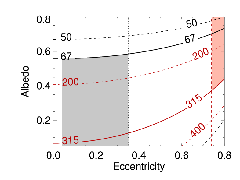
Figure 3.— The outgoing flux from two Kepler targets in terms of eccentricity and albedo. Kepler-62 f in black and KOI 5737.01 in red. The contour lines denote the outgoing flux in W/m^-2, with the solid contours representing the only limiting flux value to habitability that is appropriate for that planet. The dashed vertical lines are $e_{min}$. The dotted black line is $e_{max}$ for Kepler-62 f. KOI 5737.01’s $e_{max}$ is 1. The shading represents the portion of parameter space that is potentially habitable when eccentricity constraints are invoked.

However, the situation is markedly different if the eccentricity constraints are invoked. The values of $e_{min}$ are 0.04 and 0.74 for Kepler-62 f and KOI 5737.01, respectively. Orbital stability gives $e_{max}=0.35$ for Kepler-62 f, which has been confirmed by N-body integrations in Shields et al. (2015), but KOI 5737.01 is isolated so its maximum eccentricity is set only by orbits that intersect the host star. In Fig. 3, the vertical dashed lines represent $e_{min}$ and dotted $e_{max}$, and the shaded regions are potentially habitable. The constraints on $e$ change their likelihoods of habitability. KOI 5737.01 is habitable throughout most of the full ($A,e$) space, but in the narrow range between $e_{min}$ and 0.8, only about half of ($A,e$) pairs is habitable. Kepler-62 f’s habitable parameter space is only slightly smaller. Including $e$ constraints, the values of $H$ are 0.65 and 0.48 for Kepler-62 f and KOI 5737.01, respectively. Thus, with the eccentricity constraints, Kepler-62 f is a higher priority object. It should be noted that the large value of $e_{min}$ for KOI 5737.01 could be artificially high because long cadence Kepler data do not provide robust constraints on impact parameters (Barnes, 2015). Nonetheless, this example is illustrative of how incorporating all observational constraints could change a prioritization strategy.

3. Comparative Habitability of KOIs

In this section we consider the entire Kepler sample as of 17 Aug 2015, including confirmed and unconfirmed planets, but no false positives. If a KOI has been validated, we use the “Confirmed Planets” data instead of the original KOI data. We cut this sample by requiring the equilibrium temperature $T_{eq}$, as reported by the Kepler team (which assumed $A=0.3$), to lie between 150 and 400 K and $R_{p}$ to be less than 2.5 ${\rm\,R_{\oplus}}$. These cuts are intended to be generous and identify all KOIs with a even a small chance of habitability. These cuts leave 268 KOIs, the 10 with the highest $H^{\prime}$ values are shown in Table 1, with the full table available on-line.

Figure 4 shows the conventional approach to identifying habitable planets: the semi-major axes of the planets are compared to the star’s semi-major axis limits from 1-D photochemical-climate models. Planets in the green regions are potentially habitable; those exterior are not. In this case we have used the recent HZ limits proposed by Kopparapu et al. (2013). This representation is not fully self-consistent as the HZ limits assumed specific stellar mass-radius and mass-luminosity relationships, and the inner edge is a function of planetary radius. Nonetheless, it is clear that the Kepler spacecraft has discovered numerous planetary candidates in the classical HZ. The KOIs that pass our cuts tend to be large and interior to the HZ. These features are primarily due to the well-known biases associated with transit detection as well as our liberal upper bound on albedo. The large number of small planet candidates near the HZ motivates the creation of a comparison scheme for potential habitability.

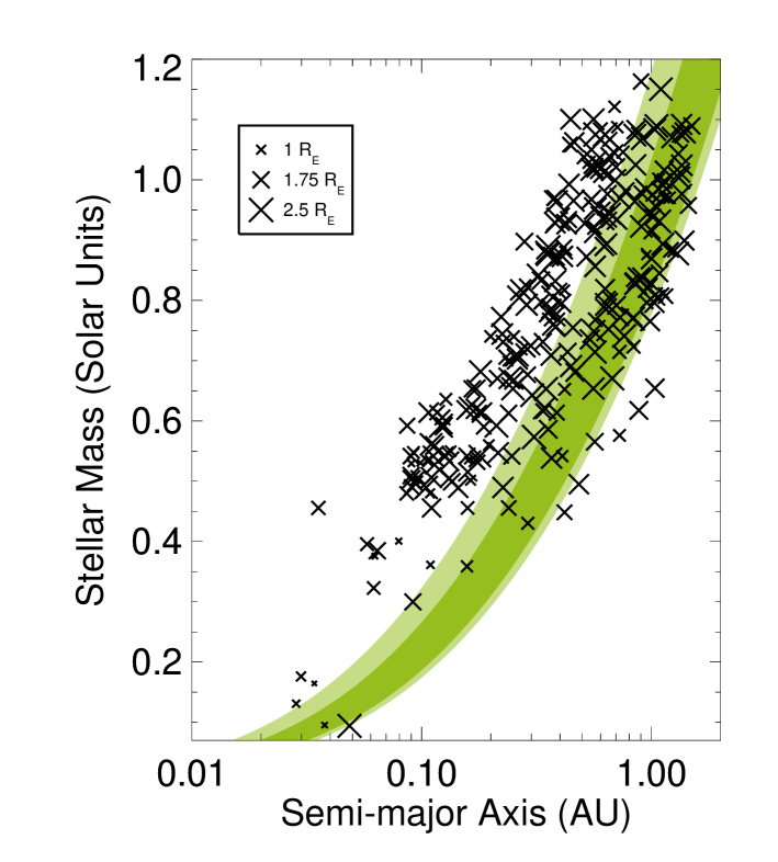
Figure 4.— Comparison of potentially habitable KOIs to the HZ. Symbol size is proportional to planetary radius as shown. Dark green is a conservative estimate of the limits of the HZ; light green optimistic (see Kopparapu et al., 2013).

Of our 268 objects, 194 had $H^{\prime}\geq 0.01$ and no object reached $H^{\prime}=1$. In Fig. 5 we plot $H^{\prime}$ against the incident stellar radiation, assuming the orbit is circular, $S_{circ}$, and scaled to the Earth’s value, $S_{\oplus}$, for all objects with $H^{\prime}>0.01$. The peak of $H^{\prime}$ occurs at $S_{circ}~{}\sim~{}0.8$, and objects near the peak should be the highest priority for follow-up, modulo observational constraints, see $\S$ 4.

Figure 5 also contains information regarding which limit is reducing $H^{\prime}$. For $0.5\leq S_{circ}\leq 1$ both flux limits can be important. In this range $H^{\prime}$ can nearly reach unity. Objects with $S_{circ}>2.5$ have less than a 20% chance of habitability by our analysis, and generally require $A~{}~{}\hbox to0.0pt{$>$\hss}{\lower 4.30554pt\hbox{$\sim$}}~{}0.7$. For individual systems the uncertainties in $S_{circ}$ can be quite large due to large uncertainties in stellar parameters (e.g.  Kane, 2014). For the planets we consider here, the average $1\sigma$ uncertainty in $S_{circ}$ is $\pm~{}36$% and so comparative habitability of KOIs is severely hampered by poor stellar characterization and one should not place too much trust in individual $H^{\prime}$ values. Figure 5 primarily shows the trend with $S_{circ}$. Presumably closer and brighter planet-hosting stars, e.g. those discovered by, e.g. TESS, will have more tightly constrained values of $S_{circ}$.

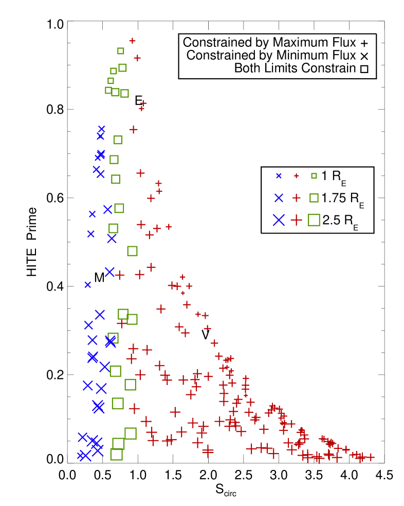
Figure 5.— $H^{\prime}$ values for KOIs as a function of the incident stellar radiation scaled to Earth’s value, and assuming a circular orbit ($S_{circ}$). Crosses indicate planets that may be uninhabitable due to too much absorbed energy, x’s too little, and open squares indicate both limiting cases are possible. Symbol size is proportional to planetary radius. The locations of Venus, Earth, and Mars are labeled with a V, E and M, respectively.

Table 1: Observed and Derived Parameters for Potentially Habitable KOIs

ID	log($g$)	$T_{eff}$	$R_{*}$	$P$	$d$	$D$	$b$	$S_{circ}$	$H$	$H^{\prime}$	$J$
	(cm/s2)	(K)	(R⊙)	(d)	(ppm)	(hr)		($S_{\oplus}$)
KOI 3456.02	4.37	6008	1.06	486.1270	120.6	9.495	0.362	0.92	0.805	0.955	11.83
KOI 7235.01	4.60	5606	0.76	299.6658	222.3	20.410	0.759	0.76	0.000	0.932	13.50
KOI 5737.01	4.46	5916	0.96	376.2425	185.7	4.064	0.328	0.99	0.480	0.916	12.61
KOI 2194.03	4.51	6038	0.92	445.2291	238.1	20.620	0.266	0.78	0.890	0.894	12.70
KOI 2626.01	4.91	3482	0.35	38.0972	1016.8	3.377	0.548	0.65	0.913	0.887	13.45
KOI 6108.01	4.39	5551	0.96	485.9230	122.9	3.756	0.452	0.61	0.000	0.865	10.90
KOI 5948.01	4.60	5776	0.76	398.5131	249.2	5.410	0.509	0.58	0.927	0.843	12.68
KOI 6425.01	4.43	5942	0.95	521.1054	231.9	14.540	0.822	0.68	0.888	0.839	13.01
Kepler-442b	4.67	4402	0.60	112.3053	614.1	5.621	0.220	0.81	0.838	0.836	13.23
Kepler-296e	4.83	3572	0.43	34.1420	852.2	3.619	0.180	1.08	0.850	0.814	13.39
…
Kepler-138d	4.89	3841	0.44	23.0881	596.7	1.946	0.924	2.25	0.000	0.233	10.29
KOI 5554.01	4.17	6113	1.28	362.2220	52.5	14.290	0.566	2.26	0.216	0.217	10.15
KOI 7587.01	4.46	5941	0.94	366.0877	494.6	11.033	0.776	1.03	0.178	0.200	10.34

The values of $H^{\prime}$ for Venus, Earth, and Mars are 0.300, 0.829, and 0.422, respectively. Several KOIs have values larger than Earth, including the confirmed planet Kepler-442 b. For reference, Kepler-62 f has $H^{\prime}=0.66$, Kepler-452 b has $H^{\prime}=0.60$, Kepler-186 f has $H^{\prime}=0.40$ and Kepler-22 b has $H^{\prime}=0.09$. Note in Table 1 that if eccentricity constraints are included, the rank of KOI 3456.02 drops significantly.

4. Future Prospects

4.1. Application to JWST

The first telescope that can measure the atmospheric composition of a terrestrial exoplanet is JWST (Deming et al., 2009; Kaltenegger & Traub, 2009; Misra et al., 2014a). Many of the details of JWST’s capabilities in regard to spectroscopic measurements of terrestrial exoplanets have been presented elsewhere (Beichman et al., 2014; Cowan et al., 2015), but have focused on the length of the observations. In other words, they assumed a target was already in hand. However, the path to discovering an appropriate target is decidedly non-trivial. The best targets will have high $H$ values, be visible year-round and have apparent brightnesses just below the saturation limit.

The first constraint we consider is apparent brightness. More photons generally means higher signal-to-noise, but below a certain apparent magnitude, the detector can saturate and invalidate the data. Beichman et al. (2014) find the minimum $J$-band magnitude is 6.9, but note that future modifications could lower it. Additional detector issues, such as the maximum number of frames that can be taken sequentially, are of second order, so we will ignore them here and refer the reader to Beichman et al. (2014). We include $J$ band magnitude in Table 1.

The second observability constraint is the total in-transit time that will be available over JWST’s lifetime. The entire sky is not always accessible, and hence higher priority should go to objects that maximize this time. The pathological case is a planet on a 1 year orbit with transits that occur when the system is occulted by the Sun. More prosaically, a system could be discovered such that during JWST’s lifetime the transits just don’t occur when the target is accessible. Thus, priority is a function of the transit ephemerides, the system’s position on the celestial sphere, and JWST’s launch date.

Without a firm launch date, it is unknown how many transits will be visible. The field of regard, or the portion of the sky that is accessible to the telescope at any given time, is limited to solar angles between $\theta_{min}=85^{\circ}$ and $\theta_{max}=135^{\circ}$, and can be computed as a function of ecliptic declination. We use the Space Telescope Science Institute’s Astronomer’s Proposal Tool to calculate the observability of potential JWST targets.

Only one confirmed planet, Kepler-138 d (KOI-314 c), has a significant $H^{\prime}$ value (0.23) and orbits a star with $J<11$. However, transit timing variations indicate a mass that is too low for a rocky composition (Kipping et al., 2014). Three Kepler planet candidates are potentially habitable, KOI 5554.01 ($H^{\prime}=0.22$), KOI 6108.01 ($H^{\prime}=0.87$) and KOI 7587.01 ($H^{\prime}=0.20$), and orbit bright stars ($J<11$). These planets are also listed in Table 1. KOI 5554.01 lies close to the maximum flux limit, but perhaps future vetting could improve its rank. We note that the Kepler team reports a stellar temperature of 6100 K, a radius of 1.3 R_⊙, but a mass of just 0.87 M_⊙. The host star has an apparent $J$ magnitude of 10.1, and is the brightest target in our list. During the 2020’s transits will occur in December and slowly slide into November at which point it is no longer accessible to JWST. Given JWST’s current configuration we find transits between 2018 and 2026 should be observable. With a 14.3 hour duration, it may be possible to acquire $\sim 125$ hours of in-transit spectroscopy of this planet, if it is validated. While a detailed study of this particular case is beyond the scope of this study, we note that at an estimated distance of 175 pc, this amount of time is unlikely to be sufficient to detect water bands with JWST (Deming et al., 2009).

KOI 7587.01 has an orbital period of 366 days and transits will occur in late June in the 2020’s. This is close to JWST observational windows, but unless modifications to the satellite’s observational constraints occur, this planet is unlikely to be observable by JWST. KOI 6108.01 has an orbital period of 486 days, which is very close to 4/3 of Earth’s orbital period. During the 2020’s transits will occur in February, June and October, but only the February transits occur in JWST’s field of regard. We conclude that KOI 5554.01 is the highest priority target for validation as it might be the only KOI that can be characterized spectroscopically with JWST.

The K2 mission has already discovered one potentially habitable super-Earth, K2-3 d (Crossfield et al., 2015). This planet has a radius of $1.5~{}{\rm\,R_{\oplus}}$ and orbits an M0V star with an orbital period of 44.6 days. We find this planet has $H^{\prime}=0.505$ and the star has a $J$ magnitude of 9.41. We include it in the online data of Table 1. Its value of $H^{\prime}$ places it 38th in terms of potential habitability, which is in the top quartile. Unfortunately due to its location on the ecliptic, K2-3 d is only accessible about 28% of the year, so although it transits 8–9 times per year, only 2–3 will be observable.

4.2. Predictions for TESS

The previous subsection highlights the challenges in detecting potentially habitable planets that are amenable to JWST spectroscopy with Kepler and K2. The TESS spacecraft (Ricker et al., 2014) has been designed explicitly to overcome these difficulties and identify habitable planets of nearby, bright stars. TESS is an all-sky transit survey with an observational footprint that mimics that of JWST, i.e. it prioritizes the ecliptic poles. In this subsection we apply our methodology to the predicted yield of TESS planets (Sullivan et al., 2015) and calculate the expected properties of its planet candidates.

For a full review of the TESS mission, consult Ricker et al. (2014). Here we review the salient points. The TESS design will favor the discovery of potentially habitable planets around early M dwarf stars with HZ orbital periods $\lesssim~{}20$ days and with photometric precision of order a few ppm. Most stars will only be monitored for 45 days, and hence earlier-type stars have HZs that are too distant for more than 2 transits to be detected, while stars later than $\approx$M4 are naturally less abundant (Henry & RECONS Team, 2009). Furthermore, the smaller relative size of M dwarfs produces deeper transits for small terrestrial planets.

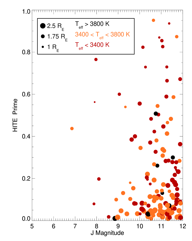
Figure 6.— Values of $H^{\prime}$ for the predicted yield of TESS planets from Sullivan et al. (2015) as a function of $J$ magnitude. Symbol size corresponds to planet size and color to the host star’s effective temperature. The colors correspond approximately to K dwarfs and earlier (black), M0–M3 dwarfs (orange), and M4 and later (red).

Recently, Sullivan et al. (2015) conducted an in-depth study to predict the exoplanet yield from TESS. They used a galactic model, the nominal TESS mission parameters, and planet occurrence rates from (Dressing & Charbonneau, 2015). They found that about 50 planets with $R<2~{}{\rm\,R_{\oplus}}$ will be discovered with $\sim 5$ in orbit around stars with $K$-band magnitudes less than 9.

Sullivan et al. (2015) also provided a complete catalog of their predicted yields with enough information to calculate $H^{\prime}$ (see their Table 6). In Fig. 6 we plot the predicted values as a function of $J$. We color code the points by $T_{eff}$ (K dwarfs in black; M0-M3 in orange; M4 and later in red), and the dot size is proportional to planetary radius. Consistent with Sullivan et al. (2015), we find 5 planets with $H^{\prime}>0.2$ and the best 2 candidates have a combined value of 1.33, suggesting if both were observed, then probably 1 would be potentially habitable, and its transmission spectrum from JWST would be very valuable.

5. Discussion

We have outlined a methodology to prioritize potentially habitable transiting exoplanets for follow-up with ground- and space-based telescopes with the explicit goal of identifying potentially habitable exoplanets amenable to transit spectroscopy. Our approach relies on published limits to habitability and assumes the bare minimum of transit and stellar data are available. The rate at which the planet’s atmosphere can cool to space, which is set by the emitted flux, has been shown to define the limits of habitability (e.g.  Kopparapu et al., 2014), and we have shown here how to calculate $F$ from the basic astronomical data.

To make our habitability comparisons, we have introduced the concept of a probabilistic $H$ that assigns a number from 0 to 1 to a planet, with larger numbers indicating a higher chance that liquid surface water is possible. This approach is markedly different from that of the classic HZ, which is essentially a binary function: potentially habitable, or not. A continuous function of habitability will become more relevant as more candidates become available. This approach is similar to that in Schulze-Makuch et al. (2011), but our method is tied directly to the observables and is based on the limits of the HZ. Torres et al. (2015) also considered the likelihood that a planet was in the HZ and that it is rocky, but they did not consider the eccentricity-albedo degeneracy, nor did they combine their probabilities into a single index. Thus, $H$ is the first physically-motivated parameter to synthesize observables into a single number that permits comparative habitability.

We have couched $H$ in terms of the absorbed (and hence emitted) flux $F$, which is a function of $e$ and $A$. The dependence on $e$ is weaker than $A$, and $e$ can often be constrained by observations, thus our results are most sensitive to our choice for the distribution of $A$. We have treated $A$ as realistically as possible, but should new insights become available, the concepts presented here should be revisited. For example, planets with high $A$ may have atmospheric properties that significantly alter the values of $F_{max}$ and/or $F_{min}$, e.g. $F_{max}=F_{max}(A)$. We encourage future work to explore the connections between $F_{max}$, $F_{min}$ and $A$.

For known KOIs we examined a wide, but plausible range of ($A,e$) combinations, ignoring limits on $e$ as the impact parameters are not well-constrained. Examination of $H^{\prime}$ and $S_{circ}$ reveals the best candidates for habitability receive 60–90% of the Earth’s solar constant, which is about the middle of the classic HZ (Kopparapu et al., 2013). Any small planet in this instellation range orbiting a bright star should immediately receive intense scrutiny for validation, stellar characterization, RV follow-up, and observations that identify the full orbital architecture of the stellar system.

We also find that KOIs with $S_{circ}~{}\geq~{}2.5$ have less than a 20% chance of being habitable and those with $S_{circ}~{}\geq~{}4$ have less than a 5% chance. Previous studies that calculated $\eta_{\oplus}$, the average number of terrestrial planets in the HZ per star, have assumed such planets are habitable (e.g.  Petigura et al., 2013). Our analysis suggests that these worlds are unlikely to be habitable unless their albedos are nearly equal to Venus’.

The continuous nature of $H$ can permit a calculation of the occurrence rate of potentially habitable planets. If we define a new parameter $\eta_{phab}$ to be the average number of “potentially habitable” planets per star, then its value is the sum of $H$ (or $H^{\prime}$) values divided by the total number of stars observed. Current technology is not sensitive enough to detect all planets of a given star, but techniques have been developed to remove the observational biases against small planets with potentially habitable orbits orbiting FGKM stars (e.g.  Catanzarite & Shao, 2011; Traub, 2012; Petigura et al., 2013; Foreman-Mackey et al., 2014). From our study, the sum of all $H^{\prime}$ values of the KOIs is 49.4, of which $\sim 10$% are likely to be false positives (Fressin et al., 2013). Our analysis suggests Kepler has discovered $\sim 45$ potentially habitable exoplanets so far. Future work could remove the observational biases and derive a value for $\eta_{phab}$.

Our approach can be applied to planets orbiting FGK dwarf stars, and many, but not late, M dwarfs. Planets orbiting late M dwarfs can have significantly more complications that impact habitability. While one can still apply our methodology to those planets, extra phenomena should be considered if possible. For example, the pre-main sequence luminosity evolution of M dwarfs can dessicate planetary surfaces (Luger & Barnes, 2015) and extreme tidal heating can trigger a runaway greenhouse (Barnes et al., 2013) or significantly alter a terrestrial planet’s evolution (Driscoll & Barnes, 2015). Tidal heating contributes to the energy budget of the atmosphere and would need to be added to Eq. (1). Expressions for tidal heating can be found in, e.g., Heller et al. (2011) and Barnes et al. (2013). Additionally, tidal circularization sculpts the $e$ distribution in the HZ for stellar masses below $\sim 0.15$ M_⊙, and hence Eq. (14) should not be used in those cases either. We note that KOI 3138.01 is a prime example of where these complications can arise. This planet candidate orbits a 0.08 M_⊙ star and has $H^{\prime}=0.74$, but it could be uninhabitable due to extreme tidal heating and/or the early super-luminous phase of its host star.

A recent study of the habitability of planets of low-mass stars explored the role of synchronous rotation and found that habitable conditions may exist at orbital distances smaller than in the traditional HZ calculations (Yang et al., 2013). That study found that a feedback can develop in which clouds form over the sub-stellar point and increase the albedo up to $\sim 0.6$. This possibility is implicitly included in our analysis as we allow for albedos larger than this value, but also reaffirms the need for better constraints on the distribution of albedos for habitable planets.

In this study we assumed flux limits based on the runaway greenhouse for planets with Earth-like inventories of water. Drier planets may remain habitable at much lower or higher fluxes. Abe et al. (2011) performed 3D models of dry planet atmospheres and found that a 1 ${\rm\,M_{\oplus}}$ planet could be habitable for $F<415$ W/m² and instellation values greater than $0.58~{}S_{\oplus}$. We did not include this possibility for three reasons. First, they did not provide flux limits at the outer edge. Second, they only considered Earth-radius planets. Third, dry planets have wider habitable limits and so we expect the peak in $H^{\prime}$ to be similar for wet planets and dry planets in terms of $S_{circ}$. Thus, the middle of the “wet” HZ of Kopparapu et al. (2013) is close to the middle of the “dry” HZ of Abe et al. (2011), and the comparative habitability of exoplanets using either method should produce similar rankings. Future work should explore a range of masses for dry planets and include the limiting flux values.

While we have focused on prioritizing targets for follow-up resources, our ranking scheme can also prioritize more in-depth theoretical analyses, such as employing 3-D global climate models (e.g.  Pierrehumbert, 2010; Wordsworth et al., 2011; Shields et al., 2015), formation models (e.g.  Raymond et al., 2004; Bond et al., 2010), and/or internal evolution (e.g.  Běhounková et al., 2011). Orbital stability should be determined through N-body simulations, especially for planets in high multiplicity systems and/or in mean motion resonances, as the Hill stability criterion does not apply in those cases and the planets can evolve chaotically for long periods of time (Barnes et al., 2015).

In this study we have explicitly assumed that the potential for habitability is purely a function of outgoing long-wavelength radiation ($\sim 1-10\micron$). This approach is the zeroeth order model for planetary habitability: Theoretical models of habitable planets must always reproduce energy balance. A thorough theoretical exploration could produce a more general “exoplanetary habitability index” that is based on the requirement of liquid surface water for a broad range of planetary compositions and structures, not emitted fluxes. Future work should develop this concept and apply it to small planets in and around the classic HZ in order to refine the priority of exoplanets for biosignature searches by future terrestrial planet characterization missions, such as LUVOIR or the High Definition Space Telescope (Dalcanton et al., 2015).

The timescale for life to arise is also important in the search for life in the unvierse. In general this timescale is unknown, but can be crudely constrained by Earth’s evolution, which included the unlikely Moon-forming impact and an orbital instability in the outer Solar System (Gomes et al., 2005). For planets in the HZs of FGK stars, the interval between the stellar birth and the last giant impact is $\sim 100$ Myr (Kokubo & Ida, 1998; Raymond et al., 2004). These events melted the entire Earth’s surface for up to several Myr (Zahnle et al., 2015) and most likely sterilized our planet. Thus, this value is a reasonable choice for the minimum age of a potentially habitable planet, and so, if available, the stellar age should be used as another data point for assessing potential habitability.

In addition to theoretical simplifications, we also do not include any uncertainties in our analysis. Stellar parameters are notoriously difficult to constrain, which can often lead to significant uncertainty in the physical and orbital properties of the planet (Gaidos, 2013; Kane, 2014). One should also propagate uncertainties when calculating $H$, possibly using a Markov chain Monte Carlo approach that produces quantified posterior distributions (e.g.  Kundurthy et al., 2011). This investigation is largely conceptual, but including uncertainties would be essential to properly allocate follow-up resources.

Planets with large values of $A$ likely have thick cloud and/or haze layers that reflect the stellar radiation. These features can make transit spectroscopy of near-surface atmospheric layers extremely difficult (e.g.  Pont et al., 2008; Misra et al., 2014b). Hence targets that require large values of $A$ may be poor JWST targets. Future research should explore the detectability of atmospheric gases of exoplanets that require high albedo in order to be habitable. Trace gas biosignatures that are confined to the troposphere may be below cloud and/or haze layers are probably undetectable with JWST.

In rare cases, the acceleration of the planet through transit can be measured and reveal the true value of $e$ (Barnes, 2007; Dawson & Johnson, 2012). For very high signal-to-noise and high cadence data, the changes in the durations and slopes of ingress and egress are detectable. When combined with $\Delta$, these features break the degeneracy between eccentricity and longitude of pericenter described in $\S$ 2.2. Barnes (2007) estimates that a Jupiter-mass planet that transits during the acceleration maximum will require $\sim 3$ ppm precision in the photometry and is thus a challenging observation to make. Nonetheless for high-priority targets that are not accessible to RV measurements, such photometric observations could be very valuable as they could also break the eccentricity-albedo degeneracy described in $\S$ 2.6.

Finally, we considered known and predicted potentially habitable exoplanets for JWST reconnaissance. The best KOI for JWST is 5554.01 with $J=10.1$. This system is probably too faint for planetary spectral measurements, but more investigations (including validation) are required to confirm this assessment. Some K2 targets have already been discovered orbiting brighter stars, but their locations on the ecliptic equator make any exoplanet in those fields unlikely to be worthy of JWST follow-up. Most likely, a proper target will be discovered by TESS, and, following up on Sullivan et al. (2015), we predict that if JWST obtains transit transmission spectroscopy of the 2 best planets, then 1 will be potentially habitable.

6. Conclusions

We have developed a simple metric, the habitability index for transiting exoplanets, to quantify the likelihood that a transiting exoplanet may possess liquid surface water. As opposed to the HZ, which is binary, this approach produces a continuum of values. $H$ can be used to prioritize follow-up efforts, whether they be observational or theoretical. Our approach to comparative habitability assessments parameterizes the eccentricity-albedo degeneracy by calculating the fraction of all possible ($A,e$) pairs that could produce a clement climate. We must also assess “rockiness” probabilistically based on inferences from the few planets with well-known masses and radii. Despite these assumptions, $H$ can provide more insight into a planet’s potential to support life than simply comparing its orbit to that of its host star’s HZ.

We ranked the known Kepler and K2 planets for habitability and found that several have larger values of $H$ than Earth. This does not mean these planets are “more habitable” than Earth – it means that an Earth twin orbiting a solar twin that is observed by Kepler would not have the highest probability of being habitable. The best candidates have incident radiation levels, assuming circular orbits, of 60–90% that of Earth’s. These levels are about in the middle of the HZ, which is not surprising as our flux limits are derived from the models that produced the HZ. Our method is grounded in the fundamental observables and can, when applicable, fold in eccentricity constraints, and is therefore more powerful than the HZ for transiting exoplanets.

As the first spacecraft capable of performing transit transmission spectroscopy is JWST, we also considered some of its features in relation to $H$. The detector capabilities and field of regard constraints could render planets with high values of $H$ unobservable. Thus, decisions on utilization of follow-up resources should also consider the design of telescopes capable of performing transmission spectroscopy. We specifically considered 4 candidates for JWST spectroscopy, KOI 5554.01, KOI 6108.01, KOI 7587.01 and K2-3 d, and find that even detection of water bands will be challenging for these objects. For now, the search continues for a suitable target for JWST.

The characterization of the atmosphere of a rocky exoplanet in the HZ will mark an important achievement in the history of exoplanetary science. In the near term, NASA and ESA have developed a sequence of missions that is capable of achieving this feat, but the resources required to realize this goal are substantial. The methodology described here can optimally focus these resources so that we can identify the best targets for transit transmission spectroscopy as quickly as possible.

We thank Pramod Gupta for designing the web interface that calculates the HITE, and Eric Agol, Kevin Zahnle, Rodrigo Luger, Abel Méndez, René Heller, Drake Deming, Mark Claire and the entire Virtual Planetary Laboratory for insightful discussions. This research has made use of the NASA Exoplanet Archive, which is operated by the California Institute of Technology, under contract with the National Aeronautics and Space Administration under the Exoplanet Exploration Program. This work was supported by the NASA Astrobiology Institute’s Virtual Planet Laboratory under Cooperative Agreement No. NNA13AA93A.

References

- Abe (1993) Abe, Y. 1993, Lithos, 30, 223
- Abe et al. (2011) Abe, Y., Abe-Ouchi, A., Sleep, N. H., & Zahnle, K. J. 2011, Astrobiology, 11, 443
- Arney et al. (2015) Arney, G., Meadows, V., Domagal-Goldman, S., Claire, M., & Schwieterman, E. 2015, in American Astronomical Society Meeting Abstracts, Vol. 225, American Astronomical Society Meeting Abstracts, # 224.02
- Ballard et al. (2011) Ballard, S., Fabrycky, D., Fressin, F., et al. 2011, ApJ, 743, 200
- Barclay et al. (2015) Barclay, T., Quintana, E. V., Adams, F. C., et al. 2015, ArXiv e-prints, arXiv:1505.01845
- Barnes (2007) Barnes, J. W. 2007, PASP, 119, 986
- Barnes (2015) Barnes, R. 2015, International Journal of Astrobiology, 14, 321
- Barnes et al. (2015) Barnes, R., Deitrick, R., Greenberg, R., Quinn, T. R., & Raymond, S. N. 2015, ApJ, 801, 101
- Barnes & Greenberg (2006) Barnes, R., & Greenberg, R. 2006, ApJ, 647, L163
- Barnes & Greenberg (2007) —. 2007, ApJ, 665, L67
- Barnes et al. (2009) Barnes, R., Jackson, B., Raymond, S. N., West, A. A., & Greenberg, R. 2009, ApJ, 695, 1006
- Barnes et al. (2013) Barnes, R., Mullins, K., Goldblatt, C., et al. 2013, Astrobiology, 13, 225
- Barnes & Quinn (2001) Barnes, R., & Quinn, T. 2001, ApJ, 550, 884
- Barnes et al. (2008) Barnes, R., Raymond, S. N., Jackson, B., & Greenberg, R. 2008, Astrobiology, 8, 557
- Batalha et al. (2011) Batalha, N. M., Borucki, W. J., Bryson, S. T., et al. 2011, ApJ, 729, 27
- Batalha et al. (2013) Batalha, N. M., Rowe, J. F., Bryson, S. T., et al. 2013, ApJS, 204, 24
- Beichman et al. (2014) Beichman, C., Benneke, B., Knutson, H., et al. 2014, PASP, 126, 1134
- Berger et al. (1993) Berger, A., Loutre, M.-F., & Tricot, C. 1993, Journal of Geophysical Research: Atmospheres, 98, 10341
- Berta et al. (2013) Berta, Z. K., Irwin, J., & Charbonneau, D. 2013, ApJ, 775, 91
- Bond et al. (2010) Bond, J. C., O’Brien, D. P., & Lauretta, D. S. 2010, Astrophys. J., 715, 1050
- Bonfils et al. (2013) Bonfils, X., Delfosse, X., Udry, S., et al. 2013, A&A, 549, A109
- Borucki et al. (2012) Borucki, W. J., Koch, D. G., Batalha, N., et al. 2012, ApJ, 745, 120
- Borucki et al. (2013) Borucki, W. J., Agol, E., Fressin, F., et al. 2013, Science, 340, 587
- Běhounková et al. (2011) Běhounková, M., Tobie, G., Choblet, G., & Čadek, O. 2011, ApJ, 728, 89
- Catanzarite & Shao (2011) Catanzarite, J., & Shao, M. 2011, ApJ, 738, 151
- Chambers et al. (1996) Chambers, J. E., Wetherill, G. W., & Boss, A. P. 1996, Icarus, 119, 261
- Cowan et al. (2015) Cowan, N. B., Greene, T., Angerhausen, D., et al. 2015, ArXiv e-prints, arXiv:1502.00004
- Crossfield et al. (2015) Crossfield, I. J. M., Petigura, E., Schlieder, J. E., et al. 2015, ApJ, 804, 10
- Dalcanton et al. (2015) Dalcanton, J., Seager, S., Aigrain, S., et al. 2015, ArXiv e-prints, arXiv:1507.04779
- Dawson & Johnson (2012) Dawson, R. I., & Johnson, J. A. 2012, ApJ, 756, 122
- Deming et al. (2009) Deming, D., Seager, S., Winn, J., et al. 2009, PASP, 121, 952
- Dressing & Charbonneau (2015) Dressing, C. D., & Charbonneau, D. 2015, ApJ, 807, 45
- Driscoll & Barnes (2015) Driscoll, P., & Barnes, R. 2015, AsBio, 15, 739
- Dumusque et al. (2014) Dumusque, X., Bonomo, A. S., Haywood, R. D., et al. 2014, ApJ, 789, 154
- Everett et al. (2013) Everett, M. E., Howell, S. B., Silva, D. R., & Szkody, P. 2013, ArXiv e-prints, arXiv:1305.0578
- Ford et al. (2008) Ford, E. B., Quinn, S. N., & Veras, D. 2008, ApJ, 678, 1407
- Foreman-Mackey et al. (2014) Foreman-Mackey, D., Hogg, D. W., & Morton, T. D. 2014, ApJ, 795, 64
- Fressin et al. (2013) Fressin, F., Torres, G., Charbonneau, D., et al. 2013, ApJ, 766, 81
- Gaidos (2013) Gaidos, E. 2013, ApJ, 770, 90
- Gaidos & Mann (2013) Gaidos, E., & Mann, A. W. 2013, ApJ, 762, 41
- Gladman (1993) Gladman, B. 1993, Icarus, 106, 247
- Goldblatt (2015) Goldblatt, C. 2015, Astrobiology, 15, 362
- Gomes et al. (2005) Gomes, R., Levison, H. F., Tsiganis, K., & Morbidelli, A. 2005, Nature, 435, 466
- Heller et al. (2011) Heller, R., Leconte, J., & Barnes, R. 2011, Astro. & Astrophys., 528, A27+
- Henry & RECONS Team (2009) Henry, T. J., & RECONS Team. 2009, in Bulletin of the American Astronomical Society, Vol. 41, American Astronomical Society Meeting Abstracts #213, #407.05
- Horner & Jones (2010) Horner, J., & Jones, B. W. 2010, International Journal of Astrobiology, 9, 273
- Howard et al. (2013) Howard, A. W., Sanchis-Ojeda, R., Marcy, G. W., et al. 2013, Nature, 503, 381
- Izon et al. (2015) Izon, G., Zerkle, A., Zhelezinskaya, Y., et al. 2015
- Jenkins et al. (2015) Jenkins, J. M., Twicken, J. D., Batalha, N. M., et al. 2015, AJ, 150, 56
- Joshi et al. (1997) Joshi, M. M., Haberle, R. M., & Reynolds, R. T. 1997, Icarus, 129, 450
- Kaltenegger & Traub (2009) Kaltenegger, L., & Traub, W. A. 2009, ApJ, 698, 519
- Kane (2014) Kane, S. R. 2014, ApJ, 782, 111
- Kasting et al. (1993) Kasting, J. F., Whitmire, D. P., & Reynolds, R. T. 1993, Icarus, 101, 108
- Kipping et al. (2014) Kipping, D. M., Nesvorný, D., Buchhave, L. A., et al. 2014, ApJ, 784, 28
- Kokubo & Ida (1998) Kokubo, E., & Ida, S. 1998, Icarus, 131, 171
- Kopparapu et al. (2014) Kopparapu, R. K., Ramirez, R. M., SchottelKotte, J., et al. 2014, ApJ, 787, L29
- Kopparapu et al. (2013) Kopparapu, R. K., Ramirez, R., Kasting, J. F., et al. 2013, ApJ, 765, 131
- Kraus et al. (2014) Kraus, A. L., Ireland, M. J., Cieza, L. A., et al. 2014, ApJ, 781, 20
- Kundurthy et al. (2011) Kundurthy, P., Agol, E., Becker, A. C., et al. 2011, ApJ, 731, 123
- Li et al. (2011) Li, L., Nixon, C. A., Achterberg, R. K., et al. 2011, Geophys. Res. Lett., 38, 23201
- Lissauer et al. (2011) Lissauer, J. J., Fabrycky, D. C., Ford, E. B., et al. 2011, Nature, 470, 53
- Lopez & Fortney (2014) Lopez, E. D., & Fortney, J. J. 2014, ApJ, 792, 1
- Luger & Barnes (2015) Luger, R., & Barnes, R. 2015, Astrobiology, 15, 119
- Marchal & Bozis (1982) Marchal, C., & Bozis, G. 1982, Celestial Mechanics, 26, 311
- Marcy et al. (2014) Marcy, G. W., Isaacson, H., Howard, A. W., et al. 2014, ApJS, 210, 20
- Misra et al. (2014a) Misra, A., Meadows, V., Claire, M., & Crisp, D. 2014a, Astrobiology, 14, 67
- Misra et al. (2014b) Misra, A., Meadows, V., & Crisp, D. 2014b, ApJ, 792, 61
- Moorhead et al. (2011) Moorhead, A. V., Ford, E. B., Morehead, R. C., et al. 2011, ApJS, 197, 1
- Moroz et al. (1985) Moroz, V. I., Ekonomov, A. P., Moshkin, B. E., et al. 1985, Advances in Space Research, 5, 197
- Nakajima et al. (1992) Nakajima, S., Hayashi, Y.-Y., & Abe, Y. 1992, J. Atmos. Sci, 49, 2256
- Pallé et al. (2004) Pallé, E., Goode, P. R., Montañés-Rodríguez, P., & Koonin, S. E. 2004, Science, 304, 1299
- Pepe et al. (2013) Pepe, F., Cameron, A. C., Latham, D. W., et al. 2013, Nature, 503, 377
- Petigura et al. (2013) Petigura, E. A., Howard, A. W., & Marcy, G. W. 2013, Proceedings of the National Academy of Science, 110, 19273
- Pierrehumbert (2010) Pierrehumbert, R. T. 2010, Principles of Planetary Climate
- Plavchan et al. (2014) Plavchan, P., Bilinski, C., & Currie, T. 2014, PASP, 126, 34
- Pont et al. (2008) Pont, F., Knutson, H., Gilliland, R. L., Moutou, C., & Charbonneau, D. 2008, MNRAS, 385, 109
- Quintana et al. (2014) Quintana, E. V., Barclay, T., Raymond, S. N., et al. 2014, Science, 344, 277
- Raymond et al. (2004) Raymond, S. N., Quinn, T., & Lunine, J. I. 2004, Icarus, 168, 1
- Ricker et al. (2014) Ricker, G. R., Winn, J. N., Vanderspek, R., et al. 2014, in Society of Photo-Optical Instrumentation Engineers (SPIE) Conference Series, Vol. 9143, Society of Photo-Optical Instrumentation Engineers (SPIE) Conference Series, 20
- Rogers (2015) Rogers, L. A. 2015, ApJ, 801, 41
- Schulze-Makuch et al. (2011) Schulze-Makuch, D., Méndez, A., Fairén, A. G., et al. 2011, Astrobiology, 11, 1041
- Selsis et al. (2007) Selsis, F., Kasting, J. F., Levrard, B., et al. 2007, Astro. & Astrophys., 476, 1373
- Sheets & Deming (2014) Sheets, H. A., & Deming, D. 2014, ApJ, 794, 133
- Shields et al. (2015) Shields, A. L., Barnes, R., Agol, E., & Meadows, V. 2015
- Shields et al. (2014) Shields, A. L., Bitz, C. M., Meadows, V. S., Joshi, M. M., & Robinson, T. D. 2014, ApJ, 785, L9
- Simpson (1927) Simpson, G. 1927, Mem. Roy. Met. Soc., 11, 69
- Sotin et al. (2007) Sotin, C., Grasset, O., & Mocquet, A. 2007, Icarus, 191, 337
- Sullivan et al. (2015) Sullivan, P. W., Winn, J. N., Berta-Thompson, Z. K., et al. 2015, ArXiv e-prints, arXiv:1506.03845
- Tomasko et al. (1980) Tomasko, M. G., Doose, L. R., Smith, P. H., & Odell, A. P. 1980, J. Geophys. Res., 85, 8167
- Torres et al. (2015) Torres, G., Kipping, D. M., Fressin, F., et al. 2015, ApJ, 800, 99
- Traub (2012) Traub, W. A. 2012, ApJ, 745, 20
- Van Eylen & Albrecht (2015) Van Eylen, V., & Albrecht, S. 2015, ApJ, 808, 126
- Weiss & Marcy (2014) Weiss, L. M., & Marcy, G. W. 2014, ApJ, 783, L6
- Williams & Pollard (2002) Williams, D. M., & Pollard, D. 2002, International Journal of Astrobiology, 1, 61
- Wordsworth et al. (2011) Wordsworth, R. D., Forget, F., Selsis, F., et al. 2011, ApJ, 733, L48
- Yang et al. (2013) Yang, J., Cowan, N. B., & Abbot, D. S. 2013, ApJ, 771, L45
- Zahnle et al. (2015) Zahnle, K. J., Lupu, R., Dobrovolskis, A., & Sleep, N. H. 2015, Earth and Planetary Science Letters, 427, 74
- Zerkle et al. (2012) Zerkle, A. L., Claire, M. W., Domagal-Goldman, S. D., Farquhar, J., & Poulton, S. W. 2012, Nature Geosciences, 5, 359