Eternal inflation in a dissipative and radiation environment: Heated demise of eternity

Abstract

Eternal inflation is studied in the context of warm inflation. We focus on different tools to analyze the effects of dissipation and the presence of a thermal radiation bath on the fluctuation-dominated regime, for which the self-reproduction of Hubble regions can take place. The tools we explore are the threshold inflaton field and threshold number of e-folds necessary to establish a self-reproduction regime and the counting of Hubble regions, using generalized conditions for the occurrence of a fluctuation-dominated regime. We obtain the functional dependence of these quantities on the dissipation and temperature. A Sturm-Liouville analysis of the Fokker-Planck equation for the probability of having eternal inflation and an analysis for the probability of having eternal points are performed. We have considered the representative cases of inflation models with monomial potentials of the form of chaotic and hilltop ones. Our results show that warm inflation tends to initially favor the onset of a self-reproduction regime for smaller values of the dissipation. As the dissipation increases, it becomes harder than in cold inflation (i.e., in the absence of dissipation) to achieve a self-reproduction regime for both types of models analyzed. The results are interpreted and explicit analytical expressions are given whenever that is possible.

I Introduction

One of the most peculiar consequences of inflation is the possibility of leading to a self-reproduction regime (SRR) of inflating Hubble regions (H regions), a phenomenon that became known as eternal inflation (for reviews, see, e.g., Refs. Guth2007 ; winitzki2009eternal ; guth2000inflation ). In eternal inflation the dynamics of the Universe during the inflationary phase is considered in a global perspective and refers to a semi-infinity (past finite, future infinity) mechanism of self-reproduction of causally disconnected H regions Vilenkin:1983xq ; Guth:1985ya ; Linde:1986fc ; Linde:1986fd . Looking at the spacetime structure as a whole, the distribution of H regions resembles much like that of a bubble foam. This scenario seems to be a generic feature present in several models of inflation. In recent years, eternal inflation attracted renewed attention due to several factors. One of them is the seemingly intrinsic connection between eternal inflation and extra dimensions theories, like string theory, and its multitude of possible solutions describing different false vacua, each one yielding its own low-energy constants vilenkin2007measure ; Guth2007 ; garriga2006probabilities , leading to what has been known by the “multiverse”, when combined with eternal inflation.

Collisions between pocket universes could upset in some level the homogeneity and isotropy of the bubble we live in and, therefore, lead to some detectable signature in the cosmic microwave background radiation (CMBR). This has then led to different proposals to test eternal inflation zhang2015testing ; wainwright2014simulating ; wainwright2014simulating2 ; feeney2011first ; feeney2011first2 ; aguirre2011status . Eternal inflation has also been recently studied in experiments involving analogue systems in condensed matter. For example, in Ref. smolyaninov2013experimental , an analogue model using magnetic particles in a cobalt-based ferrofluid system has been used to show that thermal fluctuations are capable of generating $2+1$-dimensional Minkowski-like regions inside a larger metamaterial that plays the role of the background of the multiverse. From the model building point of view, a relatively recent trend is to look for new models, or specific regimes in known models, where SRR may be suppressed. If eternal inflation does not take place, then its typical conceptual and predictive problems could be avoided, thus allowing the return of a more simple picture of universe evolution. For example, in Ref. mukhanov2014inflation , it is discussed as an extension of a cold inflationary scenario where some requirements are established such that a SRR could be suppressed. In Ref. kinney2014negative , the authors discuss the possibility of preventing a SRR given a negative running of the scalar spectral index on superhorizon scales, motivated by earlier results from Planck Planck2013 and by the BICEP2 experiment BICEP2 . In a more recent work brandenberger2015can , it is discussed how backreaction effects impact on the stochastic growth of the inflaton field. The authors in Ref. brandenberger2015can have concluded that for a power-law and Starobinsky inflation, the strength of the backreaction is too weak to avoid eternal inflation, while in cyclic Ekpyrotic scenarios, the SRR could be prevented.

In this work, we want to study and then establish the conditions for the presence of a SRR under the framework of the warm inflation picture Berera:1995ie . In the standard inflationary picture, usually known as cold inflation, it is typically assumed that the couplings of the inflaton field to other field degrees of freedom are negligible during inflation, becoming only relevant later on in order to produce a successful preheating/reheating phase, leading to a thermal radiation bath when the decay products of the inflaton field thermalize. In cold inflation, density fluctuations are mostly sourced by quantum fluctuations of the inflaton field lyth2009primordial . On the other case, in the warm inflation picture, it may happen that the couplings among the various fields are sufficiently strong to effectively generate and keep a quasiequilibrium thermal radiation bath throughout the inflationary phase. In this situation, the inflationary phase can be smoothly connected to the radiation dominated epoch, without the need, a priori, of a separate reheating period (for reviews, see, e.g., Refs. WIreviews1 ; WIreviews2 ). In warm inflation, the primary source of density fluctuations comes from thermal fluctuations, which originate in the radiation bath and are transferred to the inflaton in the form of adiabatic curvature perturbations warmpert1 ; warmpert2 .

We know from many recent studies ng1 ; ng2 ; Liu:2014ifa ; LAS2013 ; bartrum2014importance ; bastero2014cosmological ; Bastero-Gil:2014raa that dissipation and stochastic noise effects are able to strongly modify the inflationary dynamics. This in turn can lead to very different predictions for observational quantities, like for the tensor-to-scalar ratio, the spectral index, and nongaussianities, when compared to the cold inflation case. Thus, it is natural to expect that those intrinsic dynamic changes in warm inflation due to dissipation and the presence of the thermal radiation bath can and should potentially affect the predictions concerning eternal inflation as well.

Warm inflation has been studied only from the “local” perspective, where only the space-time region causally accessible from one worldline is described. On the other hand, the insertion of a warm inflation features in the context of a “global” picture, where the eternal inflation description becomes relevant, has been neglected so far. The different predictions of cold and warm inflation concerning the conditions for the establishment of a SRR regime could result in one more tool to select the most realistic model given appropriate observational constraints. The main question we aim to address in this paper is how the presence of dissipation, stochastic noise, and a thermal bath generated through dissipative effects during warm inflation will affect the global structure of the inflationary universe. For this, we develop a generalized eternal inflation model of random walk type in the context of warm inflation and use standard tools like the Sturm-Liouville analysis (SLA) of the Fokker-Planck equation associated with the random process and the analysis of the presence of eternal points, which allow us to verify the presence of a fluctuation-dominated range (FDR). In addition, we introduce the analysis of the threshold value of the inflaton field and the threshold number of e-folds for the existence of a FDR and the counting of Hubble regions produced during the global (warm) inflationary evolution in order to assess how warm inflation modifies typical measures of eternal inflation. In this work, we do not intend to address the known conceptual and prediction issues usually associated with eternal inflation (for a recent discussion of these issues and for the different point of views on these matters, see, e.g., Refs. Ijjas:2013vea ; Guth:2013sya ; Linde:2014nna ).

This paper is organized as follows. In Sec. II, we briefly review the basics of random walk eternal inflation in the cold inflation context. The different ways of characterizing eternal inflation, and those we will be using in this work are also reviewed. In Sec. III, the ideas of warm and eternal inflation are combined and a generalized model is described. The relevant results are discussed in Sec. IV and, finally, our concluding remarks are given in Sec. V. We also include two appendices where we give some of the technical details used to derive our results and also to explain the numerical analysis we have employed.

II Characterizing Eternal inflation: a brief exposition

Eternal inflation refers to the property of the inflationary regime having no end when we look at the spacetime structure as a whole. This scenario is a generic feature present in several inflation models, provided that certain conditions are met, as we will discuss below. Mathematically, the formulation that allow us to model eternal inflation is mostly conveniently expressed in terms of the Starobinsky stochastic inflation program, which describes the backreaction of the short wavelength modes, which get frozen at the horizon crossing, into the dynamics of the long wavelength inflaton modes original ; Starobinsky1994 . In this context, the standard equation of motion for the inflaton field $\varphi$ can be written as a Langevin-like equation of the form original

$$\dot{\varphi}=f(\varphi)+\sqrt{2D^{(2)}(\varphi)}\zeta\;,$$ (1)

where $f(\varphi)\equiv-V_{,\varphi}/(3H(\varphi))$ and $D^{(2)}(\varphi)=H^{3}(\varphi)/(8\pi^{2})$ are, respectively, the drift and diffusion coefficients, and $\zeta$ is a Gaussian noise term that accounts for the quantum fluctuations of the inflaton field, whose correlation function is given by $\langle\zeta(t)\zeta(t^{\prime})\rangle=\delta(t-t^{\prime})$. In de Sitter spacetime, we can show that the inflaton fluctuations grow linearly as a function of time PhysRevD.26.1231 ; Linde1982335 ; Starobinsky1982175 ,

$$\langle\varphi^{2}(t+\Delta t)\rangle-\langle\varphi^{2}(t)\rangle\sim\frac{H^{3}}{4\pi^{2}}\Delta t\;.$$ (2)

It is assumed that when subhorizon modes cross the horizon ($\sim H^{-1}$), they become classical quantities in a sufficiently small time interval. Consequently, the large-scale dynamics for the inflaton can be seen as a random walk with a typical stepsize $\sim H/(2\pi)$ in a time interval $\sim H^{-1}$. Defining $\varphi_{d}(t)$ as the deterministic dynamics for the inflaton field, we can distinguish between two typical regimes: i) if $\dot{\varphi}_{d}H^{-1}$ dominates over the fluctuations, the slow-roll evolution of the inflaton field is essentially deterministic; ii) in the opposite case, when the fluctuations dominate over the $\dot{\varphi}_{d}H^{-1}$ term, then the inflaton dynamics can be treated as a random walk and we have a FDR. In the FDR, random fluctuations of the inflaton field may advance or delay the onset of the reheating phase in different regions, avoiding global reheating. Given a value of $\varphi$ that is nearly homogeneous in a region of the order of magnitude of the horizon size (known as Hubble region or H region) and has a value that satisfies the FDR, this H region will expand, generating seeds for new H regions, and this process goes on indefinitely towards future. In a sense, one can say that a requirement for the presence of a SRR is that the inflationary dynamics goes through a FDR.

The fluctuations of the inflaton field are represented in Eq. (1) by the noise term $\sqrt{2D^{(2)}(\varphi)}\zeta$, whereas the term $f(\varphi)$ represents the deterministic evolution. Therefore, a FDR occurs when the following condition is satisfied winitzki2009eternal :

$$\frac{|f(\varphi)|}{H}\ll\sqrt{\frac{2D^{(2)}}{H}}\;.$$ (3)

More precisely, the time evolution of the inflaton field is strongly nondeterministic while the diffusion term dominates over the drift one. We call Eq. (3) the FDR condition.

The FDR condition provides the values of the inflaton field for which a FDR is set, serving as a sufficient tool to look for the presence of eternal inflation. However, we will see in the following sections that as we leave the cold inflation context and generalize the FDR condition to warm inflaton, it acquires a nontrivial dependence in the thermal bath variables, and we need to introduce additional tools in order to appreciate the presence of eternal inflation. For the sake of comparison, we perform these approaches for both cold and warm inflation.

In the following subsections, we introduce the SLA of the Fokker-Planck equation and the analysis of the presence of eternal points, which are generic for both cold and warm inflation cases.

II.1 Fokker-Planck equation

Statistical properties of $\varphi$ can be obtained through the probability density function $P(\varphi,t)d\varphi$. This is a function that describes the probability of finding the inflaton field at a value $\varphi$ at time $t$, where the values of $\varphi$ are measured in a worldline randomly chosen at constant ${\bf x}$ coordinates in a single H region. $P(\varphi,t)$ is known as the comoving probability distribution and satisfies the following Fokker-Planck equation:

$$\frac{\partial P}{\partial t}=\frac{\partial}{\partial\varphi}\left[-D^{(1)}(\varphi)P+\frac{\partial}{\partial\varphi}\left(D^{(2)}(\varphi)P\right)\right]\;.$$ (4)

However, when one is interested in the global perspective, one has to consider the volume weighted distribution, $P_{V}(\varphi,t)$, where the volume contains many H regions. The expression $P_{V}(\varphi,t)d\varphi$ is defined as the physical three-dimensional volume $\int\sqrt{-g}d^{3}{\bf x}$ of regions having the value $\varphi$ at time $t$. This distribution satisfies the equation

$$\frac{\partial P_{V}}{\partial t}=\frac{\partial}{\partial\varphi}\left[-D^{(1)}(\varphi)P_{V}+\frac{\partial}{\partial\varphi}\left(D^{(2)}(\varphi)P_{V}\right)\right]+3H(\varphi)P_{V}\;,$$ (5)

where the fundamental difference in relation to Eq. (4) is the presence of the $3H(\varphi)P_{V}$ term, which describes the exponential growth of a three-dimensional volume in regions under inflationary expansion. We can also write a Fokker-Planck equation for the distribution $P_{V}(\varphi,t)$, normalized to unity, $P_{P}(\varphi,t)\equiv P_{V}(\varphi,t)/\left\langle\exp{\left(3\int dtH\right)}\right\rangle$, but it is sufficient for our analysis to work with $P_{V}$.

To completely specify the probability distribution function, one needs to assume certain boundary conditions. Exit boundary conditions, $\frac{\partial}{\partial\varphi}\left[D^{(2)}(\varphi)P\right]_{\varphi=\varphi_{c}}=0$ and $\frac{\partial}{\partial\varphi}\left[D^{(2)}(\varphi)P_{V}\right]_{\varphi=\varphi_{c}}=0$, and/or absorbing boundary condition, $P(\varphi_{c})=0$, are typically imposed at the end of inflation (reheating boundary or surface), $\varphi_{c}=\varphi_{f}$, and at the beginning of inflation, $\varphi_{c}=\varphi_{i}$, where $\varphi_{i}$ and $\varphi_{f}$ are, respectively, the initial and final values for the inflaton field. In our analysis, we will adopt the Itô ordering and the proper-time parametrization (for discussions concerning gauge dependence and factor ordering issues, see, for example, Ref. Winitzki1996 ).

A general overdamped Langevin equation of the form

$$\dot{\varphi}=f(\varphi)+g_{1}(\varphi)\zeta_{1}(t)+g_{2}(\varphi)\zeta_{2}(t)\;,$$ (6)

with noises $\zeta_{1}$ and $\zeta_{2}$ satisfying

$$\langle\zeta_{i}(t)\rangle=0\leavevmode\nobreak\ ,$$

$$\langle\zeta_{i}(t)\zeta_{i}(t^{\prime})\rangle=\delta(t-t^{\prime})\leavevmode\nobreak\ ,$$

$$\langle\zeta_{i}(t)\zeta_{j}(t^{\prime})\rangle=\theta\delta(t-t^{\prime})\;,$$ (7)

possesses an associated Fokker-Planck equation (following the Itô prescription) given by

$$\frac{\partial}{\partial t}P(\varphi,t) =-\frac{\partial}{\partial\varphi}\left[D^{(1)}P(\varphi,t)\right]+\frac{\partial^{2}}{\partial\varphi^{2}}\left[D^{(2)}P(\varphi,t)\right]$$

$$=-\frac{\partial}{\partial\varphi}\left\{D^{(1)}P(\varphi,t)-\frac{\partial}{\partial\varphi}\left[D^{(2)}P(\varphi,t)\right]\right\}\;.$$ (8)

The drift and diffusion coefficients are given, respectively, by madureira1996giant

$$D^{(1)}=f(\varphi)\;,$$

$$D^{(2)}=\frac{g_{1}(\varphi)^{2}}{2}+\theta g_{1}(\varphi)g_{2}(\varphi)+\frac{g_{2}(\varphi)^{2}}{2}\;.$$ (9)

II.2 Sturm-Liouville analysis

Looking at the Fokker-Planck equation, Eq. (II.1), we can identify the following differential operator:

$$L_{FP} = -\frac{\partial}{\partial\varphi}D^{(1)}(\varphi)-D^{(1)}(\varphi)\frac{\partial}{\partial\varphi}$$ (10)

$$+ \frac{\partial^{2}}{\partial\varphi^{2}}D^{(2)}+\frac{\partial}{\partial\varphi}D^{(2)}\frac{\partial}{\partial\varphi}+D^{(2)}\frac{\partial^{2}}{\partial\varphi^{2}}\;,$$

which, in the light of Eq. (II.1), allow us to write the differential equation

$$L_{FP}P(\varphi,t)=-\frac{\partial}{\partial\varphi}S(\varphi,t)\;,$$ (11)

where $S(\varphi,t)=D^{(1)}P(\varphi,t)-\frac{\partial}{\partial\varphi}\left[D^{(2)}P(\varphi,t)\right]$ is called the probability current.

We can write the general solution of the Fokker-Planck equation, Eq. (11), as

$$P(\varphi,t)=\sum_{n}C_{n}P_{n}(\varphi)e^{\Lambda_{n}t}\;,$$ (12)

where $C_{n}$ are constants and the sum is performed over all eigenvalues $\Lambda_{n}$ of the operator given by Eq. (10), which in turn satisfies the following eigenvalue equation:

$$L_{FP}P_{n}(\varphi)=\Lambda_{n}P_{n}(\varphi)\;.$$ (13)

It is easy to show that the operator $L_{FP}$, Eq. (10), is not Hermitian. By redefining variables such that Winitzki1996 ; winitzki2009eternal ,

$$\varphi\rightarrow\int d\sigma\sqrt{D^{(2)}(\sigma)}\;,$$

$$\frac{\partial}{\partial\varphi}\rightarrow\frac{1}{\sqrt{D^{(2)}(\varphi)}}\frac{\partial}{\partial\sigma}\;,$$

$$P_{n}(\varphi)\rightarrow\frac{1}{D^{(2)}(\sigma)^{3/4}}\exp{\left[\frac{1}{2}\int d\sigma\frac{D^{(1)}(\sigma)}{\sqrt{D^{(2)}(\sigma)}}\right]}\psi_{n}(\sigma)\;,$$ (14)

we can transform the original Fokker-Planck equation into a Sturm-Liouville problem. The advantage of this transformation rests in the fact that the Sturm-Liouville operator is self-adjoint on the Hilbert space, and its eigenvalues $\lambda$, $L_{SL}y_{\lambda}(x)=\lambda y_{\lambda}(x)$, are real. Inserting the above transformations in Eq. (13), we obtain a new eigenvalue equation, which can be expressed as

$$\frac{\partial^{2}}{\partial\sigma^{2}}\psi_{n}(\sigma)-V_{S}(\sigma)\psi_{n}(\sigma)=\Lambda_{n}\psi_{n}(\sigma)\;,$$ (15)

where the effective potential $V_{S}$ is defined in terms of the drift $D^{(1)}(\sigma)$ and diffusion $D^{(2)}(\sigma)$ coefficients. For our purpose, we write $V_{S}$ in terms of the old variable $\varphi$, which gives

$$V_{S}(\varphi)=\frac{3}{16}\frac{(D^{(2)}_{,\varphi})^{2}}{D^{(2)}}-\frac{D^{(2)}_{,\varphi\varphi}}{4}-\frac{D^{(2)}_{,\varphi}D^{(1)}}{2D^{(2)}}+\frac{D^{(1)}_{,\varphi}}{2}+\frac{(D^{(1)})^{2}}{4D^{(2)}}\;.$$ (16)

One can interpret Eq. (15) formally as a time independent Schrödinger equation describing a particle in a potential $V_{S}$ with energy values $-\Lambda_{n}$. The same procedure can be performed for the volume weighted distribution $P_{V}(\varphi,t)$ equation, which is given by

$$\left[L_{FP}+3H\right]P_{V_{n}}(\varphi)=\Lambda^{\prime}_{n}P_{V_{n}}(\varphi)\;,$$ (17)

which adds a $-3H$ term to the effective potential, Eq. (16).

To analyze the Fokker-Planck equation, one can make use of the Sturm-Liouville theory Winitzki1996 ; winitzki2009eternal . The Schrödinger-like equation for the comoving probability distribution $P(\phi,t)$, Eq. (15), is a particular case of the general Sturm-Liouville problem. Instead of considering $P(\phi,t)$ for our analysis, it is more useful to consider the volume weighted distribution $P_{V}(\phi,t)$ due to its physical relevance. For each of these distributions, we can write the solution $\Psi(x,t)=\sum_{n}\psi_{n}(x)e^{\Lambda_{n}t}$, with energy values $E_{n}=-\Lambda_{n}$. For the distribution $P_{V}(\phi,t)$, we can write $P_{V}(\phi,t)=\sum_{n}P_{V_{n}}(x)e^{\Lambda^{\prime}_{n}t}$. If $\Lambda^{\prime}_{0}>0$ ($E^{\prime}_{0}<0$), the physical volume of the inflating regions grows with time, and eternal self-reproduction is present. Taking the boundary conditions into account, the following expression can be written for the zeroth eigenvalue Winitzki1996 ; winitzki2009eternal :

$$\Lambda_{0}=-\mbox{min}_{\psi(\sigma)}\frac{\int d\sigma\left[\left(\frac{d\psi_{n}}{d\sigma}\right)^{2}+V_{S}(\sigma)\psi_{n}^{2}\right]}{\int d\sigma\;\psi_{n}^{2}}\,.$$ (18)

From Eq. (18), we can see that the only possibility compatible with eternal self-reproduction is if there is at least a range $\sigma_{1}<\sigma<\sigma_{2}$, such that the effective potential $V_{S}(\sigma)$ is negative. Since the magnitude of the derivative term in the numerator of Eq. (18) is not determined, the SLA of the Fokker-Planck equation cannot ensure the presence of eternal inflation. However, when we analyze $V_{S}(\sigma)$ together with the FDR condition, Eq. (3), a conclusive SLA can be performed.

For the numerical analysis performed in Sec. IV, we found that it is more convenient to analyze $V_{S}(\sigma)$ in terms of the inflaton amplitude $\varphi$, instead of $\sigma$. Since inflationary dynamics is given in the variable $\varphi$, we use the functional relation between $\varphi$ and $\sigma$, given by the first expression in Eq. (II.2), to write $V_{S}$ as a function of $\varphi$.

II.3 Eternal points analysis

Finally, a third tool typically used to study the presence of eternal inflation is to look for the presence of eternal points. Eternal points are comoving worldlines x that never reach the reheating surface, i.e, are those points for which inflation ends at $t=\infty$. Therefore, if one is able to proof the existence of eternal points, eternal inflation occurs. The existence of eternal points can be addressed by solving a nonlinear diffusion equation for the complementary probability of having eternal points winitzki2009eternal

$$D^{(2)}(\varphi)\overline{X}^{\prime\prime}(\varphi)+D^{(1)}(\varphi)\overline{X}^{\prime}(\varphi)+3H(\varphi)\overline{X}(\varphi)\ln{\overline{X}(\varphi)}=0\;,$$ (19)

where prime indicates a derivative with respect to $\varphi$: ${}^{\prime}\equiv d/d\varphi$. $\overline{X}$ is related to $X$ by $X=1-\overline{X}$, where $X$ is the probability of having eternal points. Eternal points exist when there is a nontrivial solution for $X(\varphi)$. An approximate solution for Eq. (19) is obtained in the FDR neglecting the $D^{(1)}\overline{X}^{\prime}$ term when using the ansatz

$$\overline{X}(\varphi)=e^{-W(\varphi)}\;,$$ (20)

where we have assumed $W$ to be a small varying function, $W^{\prime\prime}\ll(W^{\prime})^{2}$. In terms of $W(\varphi)$, Eq. (19) takes the form

$$D^{(2)}(W^{\prime})^{2}-3HW=0\;.$$ (21)

The solution to the above equation can be formally expressed as

$$W(\varphi)=\frac{1}{4}\left(\ \int\limits_{\varphi_{\rm{th}}}^{\varphi}\sqrt{\frac{3H}{D^{(2)}}}d\varphi\right)^{2}\;,$$ (22)

where $\varphi_{\rm{th}}$ is the threshold amplitude value for the inflaton field, obtained from Eq. (3) and represents the boundary of the fluctuation-dominated range of $\varphi$ where eternal inflation ends.

III Generalizing eternal inflation in the context of warm inflation dynamics

In the first-principles approach to warm inflation, we start by integrating over field degrees of freedom other than the inflaton field. The resulting effective equation for the inflaton field turns out to be a Langevin-like equation with dissipative and stochastic noise terms. An archetypal equation of motion for the inflaton field can be written as WIreviews1 ; Berera:2007qm

$$\ddot{\Phi}({\bf x},t)+\left[3H+\Upsilon\right]\dot{\Phi}({\bf x},t)-\frac{1}{a^{2}}\nabla^{2}\Phi({\bf x},t)+V_{,\Phi}(\Phi)=\xi_{T}({\bf x},t)\;,$$ (23)

where $\Upsilon=\Upsilon(\Phi,T)$ is the dissipation coefficient, whose functional form depends on the specifics of the microphysical approach (see, e.g., Refs. Bastero-Gil2011 ; BasteroGil:2012cm for details), and $\xi_{T}({\bf x},t)$ is a thermal noise term coming from the explicit derivation of Eq. (23) and that satisfies the fluctuation-dissipation relation,

$$\langle\xi_{T}({\bf x},t)\xi_{T}({\bf x}^{\prime},t^{\prime})\rangle=2\Upsilon Ta^{-3}\delta^{(3)}({\bf x}-{\bf x}^{\prime})\delta(t-t^{\prime}).$$ (24)

Following the Starobinsky stochastic program, we perform a coarse graining of the quantum inflaton field $\Phi$, by decomposing it into short and long wavelength parts, $\Phi_{<}$ and $\Phi_{>}$, respectively,

$$\Phi({\bf x},t)=\Phi_{<}({\bf x},t)+\Phi_{>}({\bf x},t).$$ (25)

In order to define $\Phi_{<}$, a filter function $W(k,t)$ is introduced such that it eliminates the long wavelength modes ($k<aH$), resulting in

$$\Phi_{<}({\bf x},t)\equiv\phi_{q}({\bf x},t)=\int\frac{d^{3}k}{(2\pi)^{3/2}}W(k,t)\left[\phi_{\bf k}(t)e^{-i{\bf k}\cdot{\bf x}}\hat{a}_{\bf k}+\phi_{\bf k}^{*}(t)e^{i{\bf k}\cdot{\bf x}}\hat{a}^{\dagger}_{\bf k}\right]\;,$$ (26)

where $\phi_{\bf k}(t)$ are the field modes in momentum space, and $\hat{a}^{\dagger}_{\bf k}$ and $\hat{a}_{\bf k}$ are the creation and annihilation operators, respectively. The simplest filter function that is usually assumed in the literature has the form of a Heaviside function, $W(k,t)=\Theta(k-\epsilon a(t)H)$, where $\epsilon$ is a small number.

Using the field decomposition defined in Eq. (25), we obtain the following equation for the long wavelength modes:

$$\ddot{\Phi}_{>}({\bf x},t)+3H\left(1+Q\right)\dot{\Phi}_{>}({\bf x},t)-\frac{1}{a^{2}}\nabla^{2}\Phi_{>}({\bf x},t)+V_{,\phi}(\Phi_{>})=\xi_{q}({\bf x},t)+\xi_{T}({\bf x},t)\;,$$ (27)

where the quantum noise is given by

$$\xi_{q}({\bf x},t)=-\left[\frac{\partial^{2}}{\partial t^{2}}+3H\left(1+Q\right)\frac{\partial}{\partial t}-\frac{1}{a^{2}}\nabla^{2}+V_{,\phi\phi}(\Phi_{>})\right]\Phi_{<}({\bf x},t),\;$$ (28)

and $Q=\Upsilon/3H$ is the dissipative ratio. The two-point correlation function satisfied by the quantum noise is given in the Appendix A.

We are interested in a field that is nearly homogeneous inside a H region, then we can consider the approximation $\Phi_{>}({\bf x},t)\approx\varphi(t)$. In addition, we consider the slow-roll approximation to obtain a Langevin-like equation of the form of Eq. (6). From these requirements, Eq (27) gives

$$\dot{\varphi}=f(\varphi)+\sqrt{2D^{(2)}_{\rm{(vac)}}}\;\zeta_{q}(t)+\sqrt{2D^{(2)}_{\rm{(diss)}}}\;\zeta_{T}(t)\;,$$ (29)

where $\langle\zeta_{i}(t)\zeta_{i}(t^{\prime})\rangle=\delta(t-t^{\prime})$ for $i=q,T$, for the quantum and dissipative noises, respectively. In Eq. (29), the drift term is given by

$$f(\varphi)=-\frac{V_{,\varphi}(\varphi)}{3H(1+Q)},$$ (30)

while the diffusion coefficients are given by (see Appendix A, for details)

$$D^{(2)}_{\rm{(vac)}} =\frac{H^{3}}{8\pi^{2}}\left(1+2n_{\tilde{k}}\right),$$ (31)

$$D^{(2)}_{\rm{(diss)}} =\frac{H^{2}T}{80\pi}\frac{Q}{(1+Q)^{2}},$$ (32)

where $n_{\tilde{k}}$ is the statistical occupation number for the inflaton field when in a thermal bath LAS2013 , which is evaluated at the lower limit scale separating the quantum and thermal fluctuations, chosen as ${\tilde{k}}/a\approx T_{H}$, where $T_{H}=H/(2\pi)$ is the Gibbons-Hawking temperature.

Equation (29) is the warm inflationary analogous to the Starobinsky cold inflation one, Eq. (1), now accounting for the backreaction of both quantum and thermal noises (see, e.g., Ref. LAS2013 , where these equations are explicitly derived in the context of warm inflation for more details).

Equation (29) reduces to Eq. (1) in the cold inflation limit, where $Q\to 0,T\to 0,n_{\tilde{k}}\to 0$. Some other useful limiting cases of Eq. (29) are: i) the weak warm inflation (WWI) limit $Q\ll 1,\ T/H\ll 1$; ii) the weak dissipative warm inflation (WDWI) limit $Q\ll 1,\ T/H\gg 1$; and iii) the strong dissipative warm inflation (SDWI) limit $Q\gg 1,\ T/H\gg 1$. For example, writing $n_{\tilde{k}}=1/[\exp(T_{H}/T)-1]$, in the WDWI limit, we have that

$$\dot{\varphi}\approx-\frac{V_{,\varphi}(\varphi)}{3H}+\frac{H^{3/2}}{2\pi}\sqrt{2\frac{T}{T_{H}}}\zeta_{q}(t)\;,$$ (33)

while in the SDWI limit, we obtain that

$$\dot{\varphi}\approx-\frac{V_{,\varphi}(\varphi)}{3HQ}+\frac{H^{3/2}}{2\pi}\sqrt{2\frac{T}{T_{H}}}\zeta_{q}(t)\;.$$ (34)

From Eqs. (33) and (34), one notices that the drift coefficient is attenuated due to the presence of dissipation, whereas dissipation plays no significant role for diffusion in both $Q\ll 1$ and $Q\gg 1$ limits. The opposite situation happens when accounting for the effect of the temperature, which always tends to enhance the diffusion coefficient in warm inflation, while its effects on the drift term is only manifest through the dependence of the dissipation coefficient on the temperature.

The homogeneous background inflaton field is defined as the coarse-grained field integrated in a H region volume: $\phi(t)=(1/V_{H})\int d^{3}{\bf x}\ \Phi({\bf x},t)$, where $V_{H}=\frac{4\pi}{3H^{3}}$. The background equation of motion for $\phi(t)$ becomes

$$\ddot{\phi}(t)+3H(1+Q)\dot{\phi}(t)+V_{,\phi}=0\;.$$ (35)

The radiation energy density produced during warm inflation is described by the evolution equation

$$\dot{\rho}_{R}+4H\rho_{R}=\Upsilon\dot{\phi}^{2}\;,$$ (36)

where $\rho_{R}=C_{R}T^{4}$, $C_{R}=\pi^{2}g_{*}/30$ and $g_{*}$ is the effective number of light degrees of freedom. In the slow-roll regime, Eqs. (35) and (36) can be approximated to

$$3H(1+Q)\dot{\phi} \simeq-V_{,\phi}\;,$$ (37)

$$\rho_{R} \simeq\frac{3}{4}Q\dot{\phi}^{2}\;,$$ (38)

while the slow-roll conditions in the warm inflation case are given by

$$\varepsilon =\frac{1}{16\pi G}\left(\frac{V_{,\varphi}}{V}\right)^{2}<1+Q\;,$$ (39)

$$\eta =\frac{1}{8\pi G}\frac{V_{,\varphi\varphi}}{V}<1+Q\;,$$ (40)

$$\beta =\frac{1}{8\pi G}\frac{\Upsilon_{,\varphi}V_{,\varphi}}{\Upsilon V}<1+Q\;,$$ (41)

where $G=1/(8\pi M_{p}^{2}$) is the Newtonian gravitational constant and $M_{p}=m_{\rm{p}}/\sqrt{8\pi}$ is the reduced Planck mass.

In this work, we will be using in our analysis monomial forms for the inflaton, which are the chaoticlike and hilltoplike potentials. The chaoticlike potentials are defined as

$$V(\varphi)=V_{0}\left(\frac{\varphi}{M_{p}}\right)^{2n}\;,$$ (42)

where $n$ is a positive integer. The other class of potentials are the hilltop ones boubekeur2005hilltop , with potential defined as

$$V(\varphi)=V_{0}\left[1-\frac{|\gamma|}{2n}\left(\frac{\varphi}{M_{p}}\right)^{2n}\right]\;.$$ (43)

In Eqs. (42) and (43), $V_{0}=\lambda M_{p}^{4}/(2n)$ and $\gamma$ is a free parameter. Here, we will consider the cases for $n=1$ (quadratic), $n=2$ (quartic), and $n=3$ (sextic) chaotic potentials, whereas for the hilltop potential, we will study the cases for $n=1$ (quadratic) and $n=2$ (quartic), for some values of the constant $\gamma$ motivated by the recent Planck analysis for these type of potentials Planck2015 . Note that the hilltop potential, Eq. (43), is usually written in the literature as $V=\Lambda^{4}\left(1-\varphi^{p}/\mu^{p}\right)$. Thus, we identify $V_{0}=\Lambda^{4}$, $p=2n$ and $\mu^{2n}=(2n/|\gamma|)M_{p}^{2n}$ for comparison. Note that chaotic monomial potentials for the inflaton, in the cold inflation picture, are highly (for the quartic and sextic cases) or marginally (for the quadratic case) disfavored by the Planck data. However, they are still in agreement with the Planck data in the context of warm inflation (see, e.g., Ref. LAS2013 and, in particular, Ref. bartrum2014importance for a detailed analysis for the case of the quartic chaotic potential in warm inflation). This is why we have included the potentials of the form of Eq. (42) in our analysis. On the other hand, hilltop potentials are found to be in agreement with the Planck data in both cold and warm inflation pictures. Both chaotic and hilltop potentials are also representative examples of large field (chaotic) and small field (hilltop) models of inflation. We thus expect that other forms of potentials that fall into those categories should also have similar results to the ones we have obtained using the above form of potentials.

For the dissipation coefficient $\Upsilon$ appearing in the inflaton effective equation of motion, we will consider the microscopically motivated form, that is a function of the temperature and the inflaton amplitude, given by WIreviews1 ; Bastero-Gil2011 ; BasteroGil:2012cm

$$\Upsilon=C_{\varphi}\frac{T^{3}}{\varphi^{2}}\;,$$ (44)

where $C_{\varphi}$ is a dimensionless dissipation parameter that depends on the specifics of the interactions in warm inflation. The dissipation coefficient Eq. (44) is obtained in the so-called low temperature regime for warm inflation. For example, this form of dissipation can be derived for the case of a supersymmetric model for the inflaton and the interactions, whose superpotential is of the form, $W=g\Phi X^{2}/2+hXY_{i}^{2}/2$, with chiral superfields $\Phi$, $X$, and $Y_{i}$, $i=1,...,N_{Y}$. In the regime where the $X$ fields have masses larger than the temperature and $Y_{i}$ are light fields, $m_{Y}\ll T$, we have that BasteroGil:2012cm : $C_{\varphi}\simeq 0.02h^{2}N_{Y}$.

It is worth to call attention to the fact that depending on the chosen initial conditions for $\varphi$ and $Q$, inflation can begin in some dissipative regime and end in another one. In chaotic inflation, $Q$ is a quantity that always increases with time. If one starts at the WWI or WDWI regimes, it is possible to occur a dynamical transition to the SDWI regime as the dynamics proceeds. For example, if the system starts in the WDWI regime, there are two possibilities: the system remains in the WDWI regime until the end of inflation, or it enters in the SDWI regime before its end. Therefore, if these dissipative dynamical transitions occur, the only natural direction is WWI$\rightarrow$WDWI$\rightarrow$ SDWI. On the other hand, in the case of hilltop inflation, it can happen that $Q$ decreases with time. Thus, transitions between regimes can occur in the opposite direction to that in the case of chaotic inflation: SDWI$\rightarrow$WDWI$\rightarrow$ WWI.

In warm inflation, dissipation and temperature effects can enhance or suppress eternal inflation depending on the regime we are analyzing. On one hand, we expect that thermal fluctuations, similar to the role played by quantum fluctuations in cold inflation, should enhance eternal inflation. But dissipation can act in the opposite direction, by damping the fluctuations and regulating the rate at which energy from the inflaton field is transferred to the radiation bath, acting as a suppressor of eternal inflation. In our numerical results, we will see the nontrivial effects from these two opposite quantities, which can be expressed in terms of the dissipation ratio $Q=\Upsilon/(3H)$ and the temperature ratio $T/H$. For convenience, these quantities are expressed in terms of their values at a horizon crossing, since this is the point we can make contact with observational constraints. For instance, the primordial power spectrum at a horizon crossing can be written as bartrum2014importance ; LAS2013

$$\Delta_{{\cal R}}^{(\rm{tot})}=\Delta^{(\rm{vac})}_{\rm{T}}+\Delta^{(\rm{diss})}=\left(\frac{H_{*}}{\dot{\phi}}\right)^{2}\left(\frac{H_{*}}{2\pi}\right)^{2}\left[1+2n_{*}+\left(\frac{T_{*}}{H_{*}}\right)\frac{2\sqrt{3}\pi Q_{*}}{\sqrt{3+4\pi Q_{*}}}\right]\;,$$ (45)

where $\Delta^{(\rm{vac})}_{\rm{T}}=\Delta^{(\rm{vac})}\left(1+2n_{*}\right)$ is the vacuum power spectrum of cold inflation $\Delta^{(\rm{vac})}$ with the enhancement due to a nonvanishing statistical distribution for the inflaton field in the thermal bath, $n_{*}\equiv n_{k_{*}}$. The term $\Delta^{(\rm{diss})}$ is the contribution to the power spectrum due to dissipation. All quantities in Eq. (45) are evaluated at the scale of a horizon crossing, with $k_{*}=a_{*}H_{*}$. We will assume that the distribution function $n_{k_{*}}$ for the inflaton is that of thermal equilibrium and, thus, is given by the Bose-Einstein distribution form, $n_{k_{*}}=1/[\exp(H_{*}/T_{*})-1]$. This assumption obviously depends on the details of the microphysics involved during warm inflation. Some physically well motivated interactions of the inflaton field with other degrees of freedom during warm inflation, that are able to bring the inflaton to thermal equilibrium with the radiation bath, have been discussed in Refs. BasteroGil:2012cm ; bartrum2014importance . In this work we will not consider further these possible details involving model building in warm inflation, but we will consider both possibilities, of an inflaton in thermal equilibrium, thus with a Bose-Einstein distribution form, and also the case where the inflaton might not be in thermal equilibrium with the radiation bath, in which case, it might have a negligible statistical distribution $n_{k}\approx 0$. Note that in the limit $(Q_{*},T_{*},n_{*})\rightarrow 0$, one recovers the standard cold inflation primordial spectrum as expected, $\Delta_{{\cal R}}=H^{4}/(4\pi^{2}\dot{\phi}^{2})$.

Recently bastero2014cosmological , it was also shown that by accounting for noise effects in the radiation bath in the perturbation expressions, there can be an additional enhancement of the spectrum in the dissipation term in Eq. (45) by a factor of ${\cal O}(40)$, giving

$$\Delta^{(\rm{diss})}\to\Delta^{(\rm{diss})}_{\rm{RN}}\approx\left(\frac{H_{*}}{\dot{\phi}}\right)^{2}\left(\frac{H_{*}}{2\pi}\right)^{2}\frac{T_{*}}{H_{*}}\frac{80\sqrt{3}\pi Q_{*}}{\sqrt{3+4\pi Q_{*}}}\;.$$ (46)

For the numerical analysis shown in the next section, we will consider the power spectrum given by Eq. (45), but we also consider the correction (46) due to the possibility of extra random terms in the full perturbation equations. This, together with the considerations on $n_{k}$ explained above, will help us to better assess the effects that these contributions have on the emergence of eternal inflation in warm inflation.

The expression for the primordial spectrum given above, Eq. (45), or with the correction given by Eq. (46) is a good fit for the complete numerical result obtained from the complete set of perturbation equations in warm inflation bastero2014cosmological for small values of $Q_{*}\lesssim 0.1$. In our numerical studies, we will restrict the analysis up to this value of dissipation ratio, though it could be extended to larger values of $Q_{*}$ by coupling the equations to those of the full perturbation equations, but we refrain to do this given the numerical time consuming involved. Besides, the analysis for $Q_{*}\lesssim 0.1$ will already suffice to make conclusions on the nontrivial effects that dissipation, noise, and the thermal radiation bath will have in the emergence of a SRR in warm inflation.

Given the primordial spectrum, the model parameters, including those for the inflaton potentials we consider in this work, Eqs. (42) and (43), are then constrained such that they satisfy the amplitude of scalar perturbations, $\Delta_{{\cal R}}\simeq 2.25\times 10^{-9}$, in accordance to the recent data from Planck Planck2015 .

Note that from the evolution equations, Eqs. (35) and (36), with $\Upsilon$ defined by Eq. (44), and the constraint on the inflaton potential given by the normalization on the amplitude of the primordial spectrum, one obtains a functional relation between $Q_{*}$ and $T_{*}/H_{*}$. In Fig. 1, we plot the functional relation between $T_{*}/H_{*}$ and $Q_{*}$. In this figure, we also consider the cases where the particle distribution is given by $n_{k}=0$ and where radiation noise contribution to the power spectrum is taken into account, for future reference. It is important to highlight that the curves $T_{*}/H_{*}\times Q_{*}$ are approximately potential independent and they are also only mildly dependent on $g_{*}$. Thus, Fig. 1 also represents the functional relation for the hilltop potentials used in the analysis done in the next section.

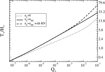
Figure 1: $T_{*}/H_{*}$ as a function of $Q_{*}$. The results are shown for two particular choices of the particle distribution, $n_{k}=0$ and for $n_{k}=n_{\rm{BE}}$, and by also accounting for the effects of the radiation noise correction in the power spectrum, Eq. (46) and in the absence of these effects, Eq. (45).

Given the relation between $T_{*}/H_{*}$ and $Q_{*}$, we are free to choose one of these variables when presenting our analysis. We choose $Q_{*}$, since it is the most transparent one, and for the corresponding values of $T_{*}/H_{*}$ for each value of $Q_{*}$ in the analysis, the reader is referred to consult the results of Fig. 1. Thus, the effects of $Q$ and $T$ on the establishment of a SRR can be adequately addressed and contrasted with the cold inflation case. Further details about the way we perform the numerical analysis are also explained in Appendix B.

In the particular case of Eq. (29), we consider the thermal and quantum noises as uncorrelated ones, since they have distinct origins (see, e.g., Ref. LAS2013 ). This corresponds to assume that the noises in Eq. (6) are uncorrelated, i.e, $\theta=0$. Then, comparing the Langevin equations given by Eq. (6) with Eq. (29) and the coefficients given by Eq. (II.1) with Eqs. (30) and (31), the drift and diffusion Fokker-Planck coefficients are, respectively, given as follows:

$$D^{(1)}=-\frac{V_{,\varphi}(\varphi)}{3H(1+Q)}\;,$$ (47)

$$D^{(2)}=\frac{H^{3}}{8\pi^{2}}\left[1+2n_{\tilde{k}}+\left(\frac{T}{H}\right)\frac{\pi Q}{10(1+Q)^{2}}\right]\;.$$ (48)

Then, starting from Eq. (29), it is possible to derive a Fokker-Planck equation that preserves the form of the original model given by Eq. (4).

IV Results

To assess the effects of dissipation and thermal fluctuations on the presence or absence of a SRR, we consider the tools described in the previous section. Thus, we will be making use of the effective potential $V_{S}$, the counting of H regions, the threshold inflaton field $\phi_{\rm{th}}$, and the threshold number of e-folds $N_{\rm{th}}$ in terms of the dissipation ratio $Q$ and $T/H$. The analysis of $V_{S}$ and of the counting of H regions produced in the SRR are presented in parallel as complementary, as well as the analysis of $\varphi_{\rm{th}}$ and $N_{\rm{th}}$.

For the whole analysis, we have used the FDR condition, Eq. (3), to determine the regions of parameters for which eternal inflation occurs. This condition is our main tool of analysis, which will become more transparent represented graphically by the aforementioned variables.

In warm inflation, the analysis of $V_{S}$ and the counting of H regions are performed in the case where inflaton particles rapidly thermalize and are given by a Bose-Einstein distribution, $n_{k}=n_{\rm{BE}}$. The analysis of $\varphi_{\rm{th}}$ and $N_{\rm{th}}$, additionally consider the possibility where the inflaton particle distribution is negligible, $n_{k}=0$. It is also analyzed the case where we consider the radiation noise (RN) contribution to the power spectrum, represented by the enhancement given in Eq. (46).

It is useful to write Eq. (29) and all related quantities in terms of dimensionless variables. We introduce the following set of transformations that we will be considering throughout this work:

$$\varphi=M_{p}x,\;\;\;\;V=\lambda M_{p}^{4}v/(2n),\;\;\;\;H=\lambda^{1/2}M_{p}L/(\sqrt{6n}),$$

$$T=\lambda^{1/2}M_{p}T^{\prime}/(\sqrt{6n}),\;\;\;\;\Upsilon=\lambda^{1/2}M_{p}\Upsilon^{\prime}/\sqrt{6n},$$

$$\zeta_{T}=(6n)^{1/4}\lambda^{1/4}M_{p}^{1/2}\zeta_{T}^{\prime}/\sqrt{3},\;\;\;\;\zeta_{q}=(6n)^{1/4}\lambda^{1/4}M_{p}^{1/2}\zeta_{q}^{\prime}/\sqrt{3},$$

$$t=3t^{\prime}/(\sqrt{6n}\lambda^{1/2}M_{p}).$$ (49)

For example, in terms of the dimensionless variables defined above, the dissipation coefficient $\Upsilon$, Eq. (44) is written as

$$\Upsilon^{\prime}=\frac{C_{\varphi}\lambda}{6n}\frac{T^{\prime 3}}{x^{2}}\;.$$ (50)

The evolution of the inflaton field, Eq. (29), expressed in terms of the drift and diffusion coefficients, Eqs. (47) and (48), in terms of the dimensionless variables (49) becomes

$$\frac{\partial x}{\partial t^{\prime}}=-\frac{v_{,x}}{2nL(1+Q)}+\frac{\sqrt{3\lambda}}{6n}\frac{L^{3/2}}{2\pi}\left(1+2n_{\tilde{k}}\right)\zeta_{q}^{\prime}+\frac{\sqrt{3\lambda}}{6n}\frac{L^{3/2}}{2\pi}\left(\frac{T^{\prime}}{L}\right)\frac{\pi Q}{10(1+Q)^{2}}\zeta_{T}^{\prime}\;.$$ (51)

From Eq. (51), we find that the volume weighted probability distribution is the solution of the following dimensionless Fokker-Planck equation:

$$\frac{\partial}{\partial t^{\prime}}P_{V}(x,t^{\prime}) = \frac{\partial}{\partial x}\left[\frac{v_{,x}}{2nL(1+Q)}P_{V}(x,t^{\prime})\right]$$ (52)

$$+ \frac{\partial^{2}}{\partial x^{2}}\left\{\frac{\lambda}{12n^{2}}\frac{L^{3}}{8\pi^{2}}\left[1+2n_{\tilde{k}}+\left(\frac{T^{\prime}}{L}\right)\frac{\pi Q}{10(1+Q)^{2}}\right]P_{V}(x,t^{\prime})\right\}$$

$$+ \frac{3L}{2n}P_{V}(x,t^{\prime})\;.$$

Using the dimensionless variables introduced in Eq. (II.2) into Eq. (52), it is possible to rewrite the Fokker-Planck equation (52) into a Schrödinger-like equation, whose effective potential is given by

$$V_{S}(\sigma)=\frac{3}{16}\frac{(D^{(2)}_{,x})^{2}}{D^{(2)}}-\frac{D^{(2)}_{,xx}}{4}-\frac{D^{(2)}_{,x}D^{(1)}}{2D^{(2)}}+\frac{D^{(1)}_{,x}}{2}+\frac{(D^{(1)})^{2}}{4D^{(2)}}-\frac{3L}{2n}\;.$$ (53)

In all situations, we take into account the field backreaction on geometry, since we are primarily interested in studying the global structure of the inflationary universe.

In the next subsections, we use the SLA to extract the relevant information from the above effective potential $V_{S}$, in the cold and warm inflation cases, and for both types of inflaton potentials considered in this work, given by Eqs. (42) and (43). The analysis of $V_{S}$ is performed comparatively with the number of H regions, $\exp{(3)}\times(N_{e}-N_{\rm{th}})$, for a total number of e-folds $N_{e}>N_{\rm{th}}$, which gives the counting of H regions produced in the FDR.

We will omit the analysis of $\bar{X}$ in the warm inflation case because, as we will see in the following, this analysis is qualitatively equivalent to the one provided by $V_{S}$, while in cold inflation, we present both for the sake of completeness.

In the following, we present results for the cold inflation scenario, for each inflaton potential model considered. Thereafter, we will extend these results to include the effects of dissipation and thermal radiation in order to establish whether they can enhance or suppress eternal inflation.

IV.1 Chaotic and hilltop models in the cold inflation case

As a warm up, let us apply the methods described in Sec. II to characterize eternal inflation for the case of cold inflation, i.e., initially in the case of absence of thermal and dissipative effects. In the cold inflation case, the evolution of the inflaton field, Eq.(51) is given by

$$\frac{\partial x}{\partial t^{\prime}}=-x^{n-1}+\frac{\sqrt{3\lambda}}{6n}\frac{x^{3n/2}}{2\pi}\zeta_{q}^{\prime}\;,$$ (54)

where the dimensionless variables (49) were used. Then, the volume weighted probability distribution is the solution of the following Fokker-Planck equation:

$$\frac{\partial}{\partial t^{\prime}}P_{V}(x,t^{\prime})=\frac{\partial}{\partial x}\left[x^{n-1}P_{V}(x,t^{\prime})\right]+\frac{\partial^{2}}{\partial x^{2}}\left[\frac{\lambda}{12n^{2}}\frac{x^{3n}}{8\pi^{2}}P_{V}(x,t^{\prime})\right]+\frac{3x^{n}}{2n}P_{V}(x,t^{\prime})\;,$$ (55)

which is a particular case of Eq. (52). Using the drift and diffusion coefficients of Eq. (55) in Eq. (53), the explicit form of the effective potential $V_{S}$ is promptly obtained, for both the chaotic and the hilltop potentials.

For the chaotic model, the effective potentials for $n=1$, $n=2$, and $n=3$ become, respectively,

$$V_{S,\rm{chaotic}}^{n=1}=-\frac{3}{2}x+\frac{\lambda}{512\pi^{2}}x+\frac{3}{2}x^{-1}+\frac{24\pi^{2}}{\lambda}x^{-3}\;,$$

$$V_{S,\rm{chaotic}}^{n=2}=-\frac{\lambda}{512\pi^{2}}x^{4}-\frac{3}{4}x^{2}+\frac{5}{2}+\frac{96\pi^{2}}{\lambda}x^{-4}\;,$$

$$V_{S,\rm{chaotic}}^{n=3}=-\frac{5\lambda}{1536\pi^{2}}x^{7}-\frac{1}{2}x^{3}+\frac{7}{2}x+\frac{216\pi^{2}}{\lambda}x^{-5}\;.$$ (56)

For the hilltop model, we obtain that

$$V_{S,\rm{hillop}}^{n=1}=-\frac{3\sqrt{v}}{2}+{\frac{\gamma}{4\sqrt{v}}}+{\frac{\lambda\gamma\sqrt{v}}{256{\pi}^{2}}}+\left({\frac{5\lambda}{2048\pi^{2}\sqrt{v}}}+{\frac{1}{2{v}^{3/2}}}+{\frac{6\pi^{2}}{\lambda{v}^{5/2}}}\right)\gamma^{2}{x}^{2}\;,$$

$$V_{S,\rm{hillop}}^{n=2}=-\frac{3\sqrt{v}}{4}+\frac{3}{8}\left({\frac{\lambda\sqrt{v}}{128{\pi}^{2}}}+{\frac{1}{\sqrt{v}}}\right)\gamma{x}^{2}+\left({\frac{5\lambda}{8192{\pi}^{2}\sqrt{v}}}+{\frac{1}{4{v}^{3/2}}}+{\frac{6{\pi}^{2}}{\lambda{v}^{5/2}}}\right){\gamma}^{2}{x}^{6}\;,$$ (57)

where $v$ is typically $v\lesssim 1$ during the FDR.

From Eqs. (IV.1) and (IV.1), due to the typical smallness of $\lambda$ and $\gamma$, one observes that in both effective potentials the negative terms are dominant for high (low) values of $x$ in chaotic (hilltop) inflation. Since high (low) $x_{0}$ are the typical initial values for chaotic (hilltop) inflation, these negative terms dominate for adequate suitable values of $x_{0}$. For chaotic inflation, as inflation evolves from high $x=x_{0}$ values to smaller $x$, the positive terms of order $\mathcal{O}(\lambda^{-1})$ increase and tend to become more relevant, whereas for hilltop inflation, the terms of order $\mathcal{O}(\gamma)$ and $\mathcal{O}(\lambda^{-1}\gamma^{2})$ tend to increase as inflation evolves from small $x=x_{0}$ values to higher $x$. These positive terms continuously increase the values of $V_{S}$ to less negative ones during inflation, which proceeds until $V_{S}>0$ at the end of inflation. From Eq. (18), we have discussed that eternal inflation is possible to occur if there is an interval of $\varphi$ (i.e., $\sigma$) where $V_{S}<0$, which can be achieved for these different forms of effective potentials. For inflation beginning at an initial field configuration that respects the FDR condition, Eq. (3), we obtain a sufficiently negative $V_{S}$ for eternal inflation to occur and, as the effective potential becomes less negative, eternal inflation eventually ceases for some less negative $V_{S}$, when the FDR condition is no longer satisfied, i.e., $\left(d\psi_{n}/d\sigma\right)^{2}$ dominates over $V_{S}$ in Eq. (18).

Together with the obtained effective potentials, we use the dimensionless version of the FDR condition, Eq. (3), to obtain $x_{\rm{th}}$, which is the (threshold) value of $x$ for which the FDR ends. If the condition Eq. (3) gives a $x_{\rm{th}}$ between $x_{\rm{0}}$ and $x_{\rm{f}}$, it means that a FDR is present. In addition, for the value of $x_{\rm{th}}$ for each potential, we can obtain the respective threshold number of e-folds $N_{\rm{th}}$.

     

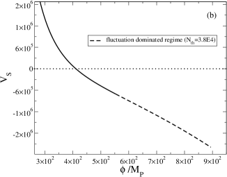
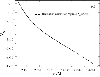
Figure 2: The effective potential $V_{S}$ for: (a) quadratic, (b) quartic, and (c) sextic chaotic inflation, respectively. The dashed curves show the fluctuation-dominated range. The values of $N_{e}$ chosen for each panel are given, respectively, by (a) $10^{7}$, (b) $10^{5}$, and (c) $10^{4}$.

     

     

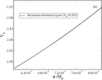
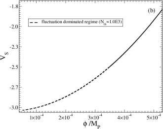
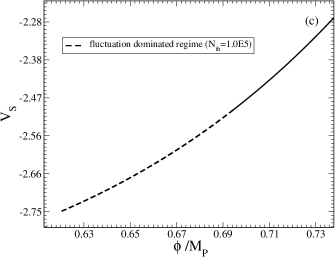
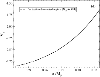
Figure 3: The effective potential $V_{S}$ for quadratic [panels (a) and (b)] and quartic [panels (c) and (d)] hilltop inflation for some representative values of $\gamma$. The dashed curves show the fluctuation-dominated range. The chosen values of $\gamma$ and $N_{e}$ for each panel are given, respectively, by (a) $10^{-3}$ and $8.4\times 10^{3}$, (b) $10^{-2}$ and $1.2\times 10^{3}$, (c) $10^{-5}$ and $1.3\times 10^{5}$, and (d) $10^{-4}$ and $10^{5}$.

In Figs. 2 and  3, we show the behavior of the effective potential $V_{S}$ for the chaotic and hilltop inflation cases, respectively. Each curve represents an inflationary evolution where we choose some $N_{e}>N_{\rm{th}}$, which means that eternal inflation occurs, and is separated in dashed and solid lines segments, which represent two distinct regimes. The dashed segment of the negative part of $V_{S}$ corresponds to the FDR, which begins at the lowermost points (the beginning of inflation and SRR, at $x=x_{0}$) and ends at where dashed and solid line segments encounter (the end of FDR, at $x=x_{\rm{th}}$). The remaining part of the curves correspond to the deterministic regime, which begins at $x=x_{\rm{th}}$ for $V_{S}<0$ and ends in the topmost point at $x=x_{\rm{f}}$, where inflation ends and $V_{S}>0$. Particularly, in Fig 2, the initial point $[x_{0},V_{S}(x_{0})]$ is always the rightmost point on the curve (recalling that $x$ decreases during the chaotic evolution), and in Fig 3, it is the leftmost point (recalling that $x$ increases during the hilltop evolution). In both cases, the vertical axis is constrained for a matter of scale, thus omitting the final value $[x_{f},V_{S}(x_{f})]$.

The dashed curves in Figs. 2 and 3 represent the $N_{e}$-$N_{\rm{th}}$ e-folds of eternal inflation where a SRR occurs, which means that for eternal inflation to happen, inflation needs to begin at an initial inflaton field value adequate to provide the sufficient number of e-folds $N_{e}>N_{\rm{th}}$. The greater the length of the dashed curves, the greater is the difference $N_{e}$-$N_{\rm{th}}$, indicating a stronger SRR. In the opposite case, the smaller we choose $N_{e}$-$N_{\rm{th}}$ the dashed line becomes smaller till it disappears for $N_{e}\leq N_{\rm{th}}$, remaining the solid curve. For eternal inflation to occur for the case of the chaotic inflation, the initial value for the inflaton field, $\varphi_{0}$, needs to be sufficiently large ($\varphi_{0}\gg M_{P}$), whereas for hilltop inflation it needs to be sufficiently small ($\varphi_{0}\ll M_{P}$), i.e., very close to the top of the potential at the origin.

The values of $x_{\rm{th}}$ given by the FDR condition (related to each $N_{\rm{th}}$ shown in the figures) are $x_{\rm{th}}=2.0\times 10^{3},\;5.5\times 10^{2},\;3.0\times 10^{2}$ in the chaotic cases (Fig. 2) for $n=1,2,3$, respectively, and in the hilltop cases (Fig. 3) by $x_{\rm{th}}=7.0\times 10^{-3}$ ($\gamma=10^{-3}$) and $x_{\rm{th}}=3.5\times 10^{-4}$ ($\gamma=10^{-2}$) for $n=1$, and $x_{\rm{th}}=0.698$ ($\gamma=10^{-5}$) and $x_{\rm{th}}=0.276$ ($\gamma=10^{-4}$) for $n=2$. In each case, we have set a value of $N_{e}$ such that a SRR is viable, i.e., $V_{S}$ exhibits a negative interval that contains a FDR.

     

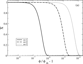
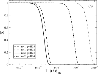
Figure 4: The probability of finding no eternal points in the chaotic [panel (a)) and hilltop (panel (b)] cold inflation cases. The chosen values of $N_{e}$ are the same ones of the previous figures for each inflation case ($n=1,2,3$) and $\gamma$.

In the Fig. 4, we show the behavior of the probability of having no eternal points for the chaotic [panel (a)] and hilltop [panel (b)] potentials. In the horizontal axis, we plot values of $x$ between $x_{\rm{0}}$ and $x_{\rm{th}}$ (FDR range), suitably parametrized by the variable $x/x_{\rm{th}}-1$ in the chaotic case and $1-x/x_{\rm{th}}$, in the hilltop case. The initial points are at the rightmost ones of the curves, indicating that eternal points are initially present ($\bar{X}\approx 0$) and vanish at the end of FDR ($\bar{X}\approx 1$).

As expected, we observe that both tools we have used to assess the presence of a SRR produce results that are compatible between them. Due to this compatibility, in the following analysis, extended to the case of warm inflation, we omit the study of eternal points for the reason of not being repetitive in performing both qualitative $V_{S}$ and eternal points analysis. In its place, we introduce the counting of H regions versus dissipation in parallel to the analysis for $V_{S}$, which is a quantitative tool and more adequate for describing the emergence of eternal inflation when considering now the effects of dissipation and radiation.

IV.2 Chaotic warm inflation

Let us initially study the case of warm inflation with the chaotic type of potentials. For the polynomial potential in the warm inflation case, the evolution of the inflaton field, Eq. (51), is given by

$$\frac{\partial x}{\partial t^{\prime}}=-\frac{x^{n-1}}{1+Q}+\frac{\sqrt{3\lambda}}{6n}\frac{x^{3n/2}}{2\pi}\left(1+2n_{\tilde{k}}\right)\zeta_{q}^{\prime}+\frac{\sqrt{3\lambda}}{6n}\frac{x^{3n/2}}{2\pi}\left(\frac{T^{\prime}}{x^{n}}\right)\frac{\pi Q}{10(1+Q)^{2}}\zeta_{T}^{\prime}\;.$$ (58)

The volume weighted probability distribution is the solution of the Fokker-Planck equation, Eq. (52), given by

$$\frac{\partial}{\partial t^{\prime}}P_{V}(x,t^{\prime}) = \frac{\partial}{\partial x}\left[\frac{x^{n-1}}{\left(1+Q\right)}P_{V}(x,t^{\prime})\right]$$ (59)

$$+ \frac{\partial^{2}}{\partial x^{2}}\left\{\frac{\lambda}{12n^{2}}\frac{x^{3n}}{8\pi^{2}}\left[1+2n_{\tilde{k}}+\left(\frac{T^{\prime}}{x^{n}}\right)\frac{\pi Q}{10(1+Q)^{2}}\right]P_{V}(x,t^{\prime})\right\}$$

$$+ \frac{3x^{n}}{2n}P_{V}(x,t^{\prime})\;.$$

From the Fokker-Planck equation, we can obtain the effective potential using Eq. (16). The expression for $V_{S}$ is too large to be presented in the text; thus, we chose to present some suitable representative results by numerical integration.

     

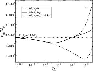
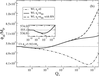
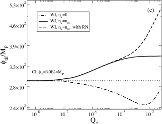
Figure 5: The threshold values of $\phi_{\rm{th}}$ versus $Q_{*}$ for the: (a) quadratic, (b) quartic, and (c) sextic chaotic inflation cases, respectively. The solid (dash-dot) curves correspond to thermal (negligible) inflaton distribution $n_{k}$ while the dashed curve corresponds to the thermal inflaton distribution and also by accounting for radiation noise effects, given according to Eq. (46).

In Fig. 5, we present the functional relation between the threshold values of the inflaton field $\varphi_{\rm{th}}$ and dissipation ratio $Q_{*}$. As expected, in all panels, we recover the cold inflation values for sufficiently small $Q_{*}$. The solid curves in the panels represent the cases where the inflaton particle distribution is given by the Bose-Einstein one. The additional dash-dotted and dashed curves represent the cases for which the inflaton particle distribution is negligible and for which the radiation noise contribution to the power spectrum is taken into account, respectively.

For the quadratic potential ($n=1$), shown in panel (a) of Fig. 5, as we increase the value of $Q_{*}$, a notable nonlinear behavior emerges: for $Q_{*}$ approximately between $10^{-12}$ and $7\times 10^{-5}$, the condition for the presence of a FDR is alleviated, since the threshold value $\varphi_{\rm{th}}$ in this interval becomes smaller than the cold inflation value (dotted curve). However, for $Q_{*}\gtrsim 7\times 10^{-5}$, the behavior is reversed and then it is noted that the establishment of a FDR is unfavored in comparison to the cold inflation case, since higher values of $\varphi_{\rm{th}}$ demand a higher initial condition for inflaton field, $\varphi_{0}$, for eternal inflation to occur.

When we account for the radiation noise effect (dashed curve), it becomes relevant only for $Q_{*}\gtrsim 2\times 10^{-4}$ and acts by increasing even more the value of $\varphi_{\rm{th}}$ in comparison to the solid curves, thus turning the FDR suppression tendency of warm inflation stronger. A simple reasoning about this behavior can be obtained analyzing Eqs. (45) and (46). Since the radiation noise contributes with a multiplicative factor $\mathcal{O}(40)$ to the dissipative power spectrum, the effects inherent to warm inflation (FDR suppression which manifests at larger values for the dissipation and thus, damping effects are stronger) are expected to be enhanced. On the other hand, in the case where $n_{k}$ is negligible (dash-dotted curve), for $Q_{*}\gtrsim 10^{-12}$ a FDR is more favored than in cold inflation, being more prominent at $Q_{*}\approx 10^{-2}$. Therefore, comparing the results shown by the dash-dotted and solid curves, one notices the deleterious role of the inflaton thermalization to the establishment of a FDR.

For the quartic potential ($n=2$), shown in panel (b) of Fig. 5, one observes the same qualitative behavior of the quadratic case. For $Q_{*}$ approximately between $10^{-10}$ and $1\times 10^{-6}$ (inset plot), a FDR is favored in comparison to cold inflation, whereas for higher values of $Q_{*}$ the presence of a FDR is harder to be achieved. Like in the quadratic case, the effect of the radiation noise on the power spectrum makes a FDR even harder to be achieved when $Q_{*}\gtrsim 10^{-4}$ and the effect of a negligible $n_{k}$ has the same FDR favoring behavior.

The sextic potential ($n=3$) case, shown in panel (c) of Fig. 5, does not favor a FDR for very small $Q_{*}$ like we have seen for the quadratic and quartic cases. The occurrence of a FDR is always disfavored for $Q_{*}\gtrsim 10^{-8}$, whereas for lower $Q_{*}$ the values of $\varphi_{\rm{th}}$ does not fall bellow the cold inflation one. However, the qualitative behavior of $\varphi_{\rm{th}}$ due to the effects of radiation noise and negligible $n_{k}$ are exactly the same of the aforementioned potentials.

Due to the qualitative similarity of the dependencies of $\varphi_{\rm{th}}$ and $N_{\rm{th}}$ on $Q_{*}$, we choose to present plots only for the former and obtain a semianalytic approximation for the functional dependence of $N_{\rm{th}}$ on $\varphi_{\rm{th}}$, which can be found to be well approximated by the expression

$$N_{\rm{th}}=\frac{1}{4n}\left(\frac{\varphi_{\rm{th}}}{M_{p}}\right)^{2}\;.$$ (60)

This solution was obtained by integrating Eqs. (80) and (81) analytically and inspecting the dominant terms. This result shows that $N_{\rm{th}}$ possesses the same qualitative behavior of $\varphi_{\rm{th}}$ with respect to making a FDR easier or harder to be achieved due to the combined effects of dissipation and thermal radiation. This means that the higher the value of $\varphi_{\rm{th}}$ we need for eternal inflation to occur, the larger is the number of e-folds of inflation required to accomplish it and vice versa. Although Eq. (60) does not contain any explicit dissipative or thermal variable, the calculation of the values of $\varphi_{\rm{th}}$ already incorporate these effects.

     

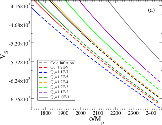
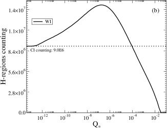
Figure 6: The effective potential $V_{S}$ as a function of $x=\phi/M_{p}$, panel (a), for some representative values of $Q_{*}$ and the counting of H regions versus $Q_{*}$, panel (b), for the quadratic chaotic inflation potential. It was taken $N_{e}=1.5\times{10}^{6}$ for the cold inflation case ($Q=0$).

     

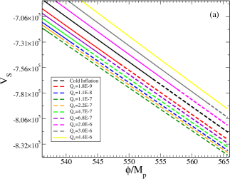
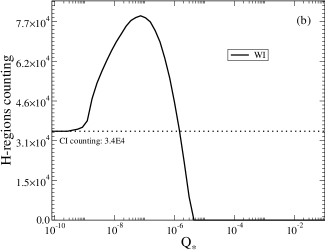
Figure 7: The effective potential $V_{S}$ as a function of $x=\phi/M_{p}$, panel (a), for some representative values of $Q_{*}$ and the counting of H regions versus $Q_{*}$, panel (b), for the quartic chaotic inflation potential. It was taken $N_{e}=4\times{10}^{4}$ for the cold inflation case ($Q=0$).

     

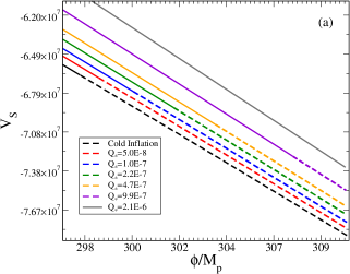
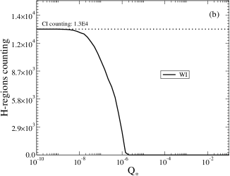
Figure 8: The effective potential $V_{S}$ as a function of $x=\phi/M_{p}$, panel (a), for some representative values of $Q_{*}$ and the counting of H regions versus $Q_{*}$, panel (b), for the sextic chaotic inflation potential. It was taken $N_{e}=8\times{10}^{3}$ for the cold inflation case ($Q=0$).

Next, we present in Figs. 6, 7, and 8, the results for the effective potential $V_{S}$ as a function of the dimensionless inflaton field [panel (a) in each of the figures] for some representative values of $Q_{*}$. We also show in parallel [panel (b) in each of the figures], the corresponding counting of H regions as a function of $Q_{*}$, for each of the chaotic inflation potential models considered. For each pair of plots for $V_{S}$ and H regions counting, we have set up an adequate initial condition $\varphi_{0}$ for the cold inflation case such that a FDR is present. This same initial condition $\varphi_{0}$ was then used to obtain all warm inflation curves of $V_{S}$ and for each point of the plots of counting of H regions. From this perspective, of same value for $\varphi_{0}$ for both cold and warm inflation cases, one can inspect whether the FDR generated in the cold inflation case is still sustained or becomes suppressed when dissipative effects are present. In the plots of $V_{S}$, the curves are separated in FDR and deterministic parts as described in the previous subsection for the cold inflation situation. One notices that the lengths of the parts corresponding to FDR increase or decrease due to the dependence of $\varphi_{\rm{th}}$ on dissipation and temperature [see Figs. (1] and (5)), thus revealing the enhancement or suppression of the FDR for each representative value of $Q_{*}$. In turn, the plots of H regions counting exhibit the number of H regions produced in the FDR parts shown in the plots for $V_{S}$.

For the quadratic potential case, shown in Fig. (6), we observe in panel (a) that the FDR dash-dotted lines increase until $Q_{*}\approx 1.1\times 10^{-7}$, which reveals a favoring tendency to eternal inflation in comparison to cold inflation. Increasing $Q_{*}$, this behavior is reversed and for $Q_{*}\gtrsim 1\times 10^{-4}$, eternal inflation is disfavored. Panel (b) corroborates this behavior in terms of the increase and subsequent decrease of the production of H regions. The corresponding value of temperature (at that particular time) for which the production of H regions decreases, i.e., eternal inflation gets disfavored, is $T_{\rm{th}}\gtrsim 1.6\times 10^{7}$ GeV. One also notes that the counting of H regions falls to zero for $Q_{*}\gtrsim 3\times 10^{-2}$. The solid grey curve in panel (a) shows an example where no FDR is present. This fall means that the chosen $\varphi_{0}$ of cold inflation is not above the threshold value to produce a FDR in warm inflation with such values of $Q_{*}$. This result is in complete consistency with the ones shown in Fig. 5(a).

The quartic potential case, shown in Fig. (7), is qualitatively similar to the quadratic case. Panel (a) shows that a FDR is more favored than in cold inflation for values $Q_{*}$ between $1.8\times 10^{-9}$ and $6.8\times 10^{-7}$, but for higher values of $Q_{*}$ the tendency is the suppression of the FDR. In panel (b), we ignore the mentioned negligible FDR favoring for very low $Q_{*}$ (no inset plot) and reiterate that for $Q_{*}\gtrsim 1\times 10^{-6}$ eternal inflation is disfavored in comparison to cold inflation as the solid curve drops below cold inflation dotted one. The corresponding value of temperature in this case is $T_{\rm{th}}\gtrsim 9.1\times 10^{10}$ GeV. For the chosen value of $\varphi_{0}$, for $Q_{*}\gtrsim 4\times 10^{-6}$, eternal inflation is completely suppressed. This result also corroborates the one shown in Fig. 5(b).

The case of a sextic potential, shown in Fig. (8), panel (a) shows that the FDR is always disfavored as we increase $Q_{*}$. For $Q_{*}\gtrsim 5\times 10^{-8}$, the lengths of the FDR curves becomes smaller in comparison to the cold inflation case until it disappears for $Q_{*}\approx 2\times 10^{-6}$. The exactly same behavior is shown in panel (b), where the production of H regions falls below the cold inflation value for corresponding values of temperature of $T_{\rm{th}}\gtrsim 3.9\times 10^{12}$ GeV, and eventually is totally suppressed. These results are again consistent to those shown in Fig. 5(c).

With the assistance of Fig. (1), we notice that the FDR favoring intervals of $Q_{*}$ obtained in the quadratic and quartic cases occur for $T/H\lesssim 1$, which is a regime between cold and warm inflation regimes, which we called WWI. For the typical warm inflation picture (where $T/H\gtrsim 1$), one observes that dissipation has the tendency to suppress the establishment of a SRR for the case of the chaotic potential models in warm inflation, in comparison to the cold inflation case.

IV.3 Hilltop warm inflation case

We now discuss and present our results for the hilltop potential case, given by Eq. (43). Equation (51) can be specialized in order to describe the inflaton dynamics under this potential

$$\frac{\partial x}{\partial t^{\prime}} = \frac{|\gamma|}{2n}\frac{x^{2n-1}}{\sqrt{1-\left(|\gamma|/2n\right)x^{2n}}(1+Q)}$$ (61)

$$+ \frac{\sqrt{3\lambda}}{6n}\frac{\left[1-\left(|\gamma|/2n\right)x^{2n}\right]^{3/4}}{2\pi}\left(1+2n_{\tilde{k}}\right)\zeta_{q}^{\prime}$$

$$+ \frac{\sqrt{3\lambda}}{6n}\frac{\left[1-\left(|\gamma|/2n\right)x^{2n}\right]^{3/4}}{2\pi}\left\{\frac{T^{\prime}}{\left[1-\left(|\gamma|/2n\right)x^{2n}\right]^{1/4}}\right\}\frac{\pi Q}{10(1+Q)^{2}}\zeta_{T}^{\prime}\;.$$

The modified Fokker-Planck equation for the volume distribution $P_{V}$, Eq. (52), can be written as

$$\frac{\partial}{\partial t^{\prime}}P_{V}(x,t^{\prime})=-\frac{\partial}{\partial x}\left[\frac{|\gamma|}{2n}\frac{x^{2n-1}}{\sqrt{1-\left(|\gamma|/2n\right)x^{2n}}(1+Q)}P_{V}(x,t^{\prime})\right]$$ (62)

$$+ \frac{\partial^{2}}{\partial x^{2}}\left\{\frac{\lambda}{12n^{2}}\frac{\left[1-\left(|\gamma|/2n\right)x^{2n}\right]^{3/2}}{8\pi^{2}}\left[1+2n_{\tilde{k}}+\left(\frac{T^{\prime}}{\sqrt{1-\left(|\gamma|/2n\right)x^{2n}}}\right)\frac{\pi Q}{10(1+Q)^{2}}\right]P_{V}(x,t^{\prime})\right\}$$

$$+ \frac{3}{2n}\sqrt{1-\left(|\gamma|/2n\right)x^{2n}}P_{V}(x,t^{\prime})\;.$$

For the analysis of the hilltop case, we set two values of $\gamma$ for each fixed $n$. Namely, we set $\gamma=10^{-3}$ and $\gamma=10^{-2}$ for $n=1$, and $\gamma=10^{-5}$ and $\gamma=10^{-4}$ for $n=2$. These values of $\gamma$ are motivated by those values considered in the recent Planck’s observational constraints on inflation based on the hilltop potential Planck2015 [note also that in Planck2015 , these values were given in terms of $\log{(\mu/M_{p})}$ instead].

     

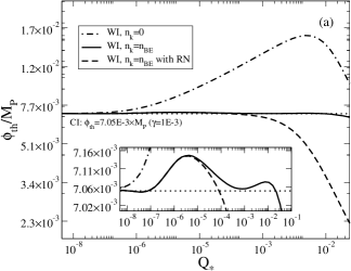
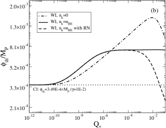
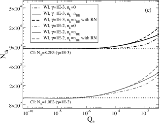
Figure 9: The threshold values of $\phi_{\rm{th}}$ [panels (a) and (b)] and $N_{\rm{th}}$ [panel (c)] versus $Q_{*}$ for the quadratic hilltop inflation potential case. Panels (a) and (b) correspond to the representative choices $\gamma=10^{-3}$ and $\gamma=10^{-2}$, respectively, whereas panel (c) covers both $\gamma=10^{-3}$ (black dashed curves) and $\gamma=10^{-2}$ (gray dashed curves) choices. The solid (dash-dot) curves correspond to thermal (negligible) inflaton distribution $n_{k}$, while the dashed curve corresponds to thermal inflaton distribution accounting for radiation noise contribution.

     

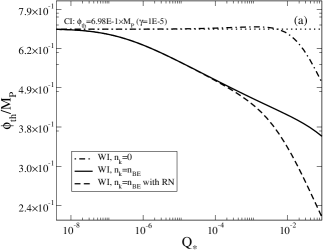
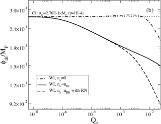
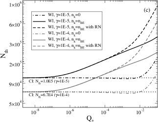
Figure 10: The same as in Fig. 9, but for the quartic hilltop inflation potential case. Panels (a) and (b) correspond to the representative choices $\gamma=10^{-5}$ and $\gamma=10^{-4}$, respectively, whereas panel (c) covers both $\gamma=10^{-5}$ (black curves) and $\gamma=10^{-4}$ (gray curves) choices. The solid (dash-dot) curves correspond to thermal (negligible) inflaton distribution $n_{k}$, while the dashed curve corresponds to thermal inflaton distribution accounting for radiation noise contribution.

In Figs. 9 and 10, we present the functional dependence of $\varphi_{\rm{th}}$ and $N_{\rm{th}}$ on the dissipation ratio $Q_{*}$ for the hilltop potential model cases. Differently to what we have seen in the chaotic potential case, for hilltop inflation the relation between $\varphi_{\rm{th}}$ and $N_{\rm{th}}$ is much more involved. Thus, we show the numerical results for both in this case. The numerical results for $\varphi_{\rm{th}}$ and $N_{\rm{th}}$ as a function of $Q_{*}$ are shown in Figs. 9 and 10 for the quadratic and for the quartic hilltop inflation potential cases, respectively. Panels (a) and (b) of each figure show the functional dependence of $\varphi_{\rm{th}}$ on $Q_{*}$ for each aforementioned choice of $\gamma$, whereas panel (c) shows the functional dependence of $N_{\rm{th}}$ on $Q_{*}$. Note that for sufficiently small values for $Q_{*}$, the cold inflation limit is recovered in all panels, as expected.

The quadratic inflation case for $\gamma=10^{-3}$ is shown in panel (a) of Fig. 9. One observes that as we increase $Q_{*}$, the value of $\varphi_{\rm{th}}$ is larger than in the cold inflation case (which is better seen in the inset plot). For hilltop inflation potential this means that the SRR is favored. In other words, since for given values of $Q_{*}$ the amplitude of the inflaton increases, i.e., moves away from the top of the potential, the region of field values between cold and warm inflation values of $\varphi_{\rm{th}}$ become now available for the SRR. Consequently, we see that a larger region of field values in warm inflation becomes suitable for leading to eternal inflation than in the cold inflation case. This favoring occurs for $Q_{*}\gtrsim 10^{-7}$ and is more pronounced at $Q_{*}\approx 4\times 10^{-6}$ and $Q_{*}\approx 10^{-2}$. However, for $Q_{*}\gtrsim 10^{-2}$, the behavior is reversed and the FDR tends to be unfavored for $Q_{*}\gtrsim 2\times 10^{-2}$. This same FDR friendly behavior happens for the quadratic case with $\gamma=10^{-2}$, shown in panel (b), which occurs for $Q_{*}\gtrsim 4\times 10^{-11}$ and stabilizes for $Q_{*}\gtrsim 5\times 10^{-5}$. In contrast, panel (c) reveals that the threshold number of e-folds $N_{\rm{th}}$ increases with dissipation for both choices of $\gamma$, which indicates that the establishment of a SRR is harder to be achieved for higher values of $Q_{*}$. These results involving $\varphi_{\rm{th}}$ and $N_{\rm{th}}$ seem contradictory to the ones seen for the chaotic inflation potential cases, where we would expect growing $\varphi_{\rm{th}}$ for growing $N_{\rm{th}}$ and vice versa. However, this apparent contradiction can be dissolved when we realize that at the same time that dissipative effects become sufficiently significant at the threshold instant to increase the values of $\varphi_{\rm{th}}$, the inflaton field value at the end of inflation, $\varphi_{\rm{f}}$, becomes smaller due to dissipation, thus increasing $N_{\rm{th}}$.

The quartic inflation cases for $\gamma=10^{-5}$ and $\gamma=10^{-4}$ are shown in panel (a) and (b) of Fig. 10, respectively. For both cases, eternal inflation is continuously suppressed as we increase $Q_{*}$ from approximately $10^{-8}$ to greater values. These behaviors are in agreement with the respective results of $N_{\rm{th}}$ given in panel (c), since we now expect that in the hilltop inflation potential lower values of $\varphi_{\rm{th}}$ will disfavor a FDR, which corresponds to greater values of $N_{\rm{th}}$.

In both Figs. 9 and 10, we also analyze the effect of a negligible inflaton particle distribution $n_{k}\approx 0$. In Figs. 9 and 10, this case is represented by dash-dotted lines in all panels. The behavior is similar to the chaotic inflation case; the curves ascend in comparison to the $n_{k}=n_{\rm{BE}}$ cases (solid curves), which again reinforces the importance of the thermalized inflation particles in the suppression of eternal inflation. In the quadratic inflation case, the establishment of a SRR is always favored, whereas in the quartic case eternal inflation is negligibly favored for very low values of $Q_{*}$ and becomes significantly suppressed for $Q_{*}\gtrsim 10^{-2}$. In both figures, we also see the effect of radiation noise contribution to the power spectrum, given according to Eq. (46). Its effect is opposite to that of negligible $n_{k}$; in the quadratic case with $\gamma=10^{-3}$, the curves descend from $n_{k}=n_{\rm{BE}}$ case for $Q_{*}\gtrsim 5\times 10^{-5}$, whereas for the quadratic case with $\gamma=10^{-2}$ and for both quartic values of $\gamma$ in the quartic potential the descent happens for $Q_{*}\gtrsim 10^{-4}$. In the quadratic case with $\gamma=10^{-3}$ ($\gamma=10^{-2}$), eternal inflation is favored for $Q_{*}\gtrsim 10^{-4}$ ($Q_{*}\gtrsim 3\times 10^{-2}$), whereas in the quartic case eternal inflation is always favored for $Q_{*}\gtrsim 10^{-4}$. This effect of the radiation noise is consistent to what we expected before in the chaotic inflation potential cases. The effect of the radiation noise is more pronounced at larger dissipation. These larger values of dissipation imply in a larger damping of fluctuations that might otherwise lead to a SRR.

     

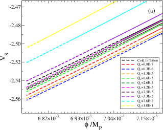
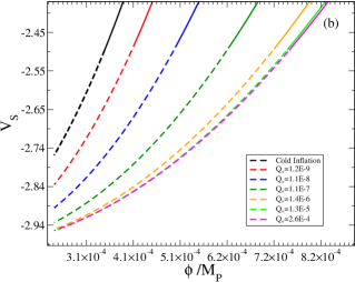
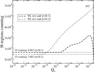
Figure 11: The effective potential $V_{S}$ as a function of $\phi$ for some representative values of $Q_{*}$ [panels (a) and (b)] and the counting of H regions versus $Q_{*}$ [panel (c)], for the quadratic hilltop inflation potential case. Panels (a) and (b) correspond to the representative choices of $\gamma=10^{-3}$ and $\gamma=10^{-2}$, respectively, whereas panel (c) covers both $\gamma=10^{-3}$ (black curve) and $\gamma=10^{-2}$ (gray curve) choices. We have chosen $N_{e}=8300$ ($\gamma=10^{-3}$) and $N_{e}=1050$ ($\gamma=10^{-2}$) for cold inflation cases.

     

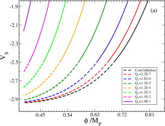
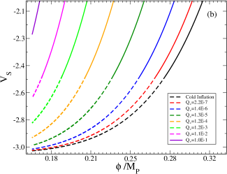
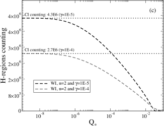
Figure 12: The same as in Fig. 11, but for the quartic hilltop inflation potential case. Panels (a) and (b) correspond to the representative choices $\gamma=10^{-5}$ and $\gamma=10^{-4}$, respectively, whereas panel (c) covers both $\gamma=10^{-5}$ (black curve) and $\gamma=10^{-4}$ (gray curve) choices. We have chosen $N_{e}=3.2\times 10^{5}$ ($\gamma=10^{-5}$) and $N_{e}=2.0\times 10^{5}$ ($\gamma=10^{-4}$) for cold inflation cases.

Finally, in Figs. 11 and 12, we present the effective potential $V_{S}$ as a function of the (dimensionless) inflaton field for some representative values of $Q_{*}$ [panels (a) and (b)] and the functional dependence of the counting of H regions on $Q_{*}$ [panel (c)], for the quadratic and quartic hilltop potentials, respectively. Panels (a) and (b) of each figure show the plots of $V_{S}$ for each choice of $\gamma$, whereas panels (c) exhibit the counting of H regions for both choices of $\gamma$. As in the chaotic inflation case, we choose suitable values of $\varphi_{0}$ for the cold inflation cases such that a FDR is present and use it to obtain the warm inflation results. We can now contrast the panel (a) of Fig. 11 with the corresponding panel (a) of Fig. 9. Observing both panels, one notes that the FDR is favored in the range $10^{-7}\lesssim Q_{*}\lesssim 2\times 10^{-2}$ in comparison to the cold inflation case and unfavored outside this range. Quantitatively, the region of the potential that corresponds to the FDR (i) increases for $10^{-7}\lesssim Q_{*}\lesssim 4\times 10^{-6}$, (ii) decreases in the range $4\times 10^{-6}\lesssim Q_{*}\lesssim 8\times 10^{-4}$, (iii) increases for $8\times 10^{-4}\lesssim Q_{*}\lesssim 8\times 10^{-3}$, and (iv) decreases for $Q_{*}\gtrsim 8\times 10^{-3}$, getting shorter than the cold inflation case for $Q_{*}\gtrsim 2\times 10^{-2}$. Analogously, we perform a joint analysis of panels (b) of Figs. 9 and 11. For $Q_{*}\gtrsim 4\times 10^{-11}$ in both panels (b), one observes that the FDR abruptly increases for increasing $Q_{*}$ until $Q_{*}\approx 10^{-6}$, where FDR continuous to increase but in a small rate. These minor details involving representative values of $Q_{*}$ are important only to contrast the corresponding panels of Figs. 9 and 11, but the main interest is in the FDR-favoring behavior that we observe for the quadratic hilltop potential case. Analogously, we contrast panels (a) and (b) of Fig. 12 to the respective panels (a) and (b) from Fig. 10. One notices that for both cases the lengths of the FDR curves decrease until it disappear for sufficiently high value of $Q_{*}$, which corresponds to the decrease of the values of $\varphi_{\rm{th}}$. The plots of the counting of H regions, given in the panels (c) of Figs. 11 and  12, mimic the results of panels (a) and (b) like in the chaotic inflation case; the amount of H regions increases when FDR is favored, decreases when it is unfavored, and falls to zero when the chosen $\varphi_{0}$ is smaller than $\varphi_{\rm{th}}$ for the specific value of $Q_{*}$. Like in the cases of the monomial chaotic potential, the corresponding values of temperature for which eternal inflation gets disfavored in comparison to cold inflation are $T_{\rm{th}}\gtrsim 4.0\times 10^{12}$ GeV for the quadratic case with $\gamma=10^{-3}$ and $T_{\rm{th}}\gtrsim 2.6\times 10^{7}$ GeV ($T_{\rm{th}}\gtrsim 1.6\times 10^{7}$ GeV) for the quartic case with $\gamma=10^{-5}$ ($\gamma=10^{-4}$), whereas for the quadratic hilltop case with $\gamma=10^{-2}$ eternal inflation is favored for the entire range of $Q_{*}$ analyzed. Once again, these plots reveal the deleterious behavior of warm inflation to the establishment of the SRR in the quartic hilltop potential case. In the quadratic hilltop potential case, however, warm inflation enhances the eternal inflation mechanism from the point of view of a fixed $\varphi_{0}$.

V Conclusions and final remarks

In this work, we have developed a generalized approach to eternal inflation of the random walk type under the framework of warm inflation. Thus, the combined effects of dissipation, the corresponding stochastic term, and the presence of a thermal radiation bath are accounted for. To understand the influence of these effects on the self-reproduction regime of the inflationary universe, we have performed a comprehensive numerical analysis of how relevant quantities that characterizes eternal inflation in the cold inflation case are modified due to the presence of dissipation and a thermal radiation bath. Since eternal inflation is mainly characterized by the presence of a FDR, the main tool we have used was a generalized condition for the occurrence of a FDR, which is used for obtaining and interpreting the results.

Taking cold inflation as a reference, within the context of the warm inflation picture we have obtained information about the functional relation between the threshold inflaton field $\varphi_{\rm{th}}$ and also for the threshold number of e-folds $N_{\rm{th}}$, in terms of the dissipation ratio $Q$ (where we used its value at the moment of horizon crossing as a reference). In addition to the usual case where the statistical occupation number is given by the Bose-Einstein distribution, i.e., assuming a thermal equilibrium distribution for the inflaton, we have also presented the cases where its particle distribution is negligible and where the dissipative power spectrum might get additional contributions due to radiation noise effects, as recently studied in Ref. bastero2014cosmological . Using the model independent relation between $Q_{*}$ and $T_{*}/H_{*}$, we were able to focus the analysis only as a function of $Q_{*}$, but always concomitantly keeping track of the influence of the temperature of the thermal bath.

In addition to the analysis of $\varphi_{\rm{th}}$ and $N_{\rm{th}}$, we have performed a SLA of the corresponding Fokker-Planck equation for the probability of having eternal inflation, translated in terms of the effective potential $V_{S}$. In parallel to the analysis of $V_{S}$, we have also analyzed the dependence of the number of H regions produced in the FDR as a function of $Q_{*}$.

We have considered as examples of inflation models, the cases of monomial potentials of the chaotic type (quadratic, quartic, and sextic chaotic inflation potentials) and hilltoplike (quadratic and quartic hilltop potentials). To study how the typical dynamics displayed in warm inflation affects eternal inflation, we have performed our analysis in a range of values for the dissipation ratio $Q_{*}$ varying from very low values (reaching the cold inflation limit) up to $Q_{*}=0.1$, where the analytical expression for the primordial spectrum is found to be in good agreement with full numerical calculations of the perturbations in warm inflation bastero2014cosmological .

For the chaotic potential cases, the dependence of both $\varphi_{\rm{th}}$ and $N_{\rm{th}}$ on $Q_{*}$ reveals that in the typical warm inflation regime dissipation and thermal fluctuations have the tendency of suppressing eternal inflation in comparison to the cold inflation case, whereas in the WWI regime, eternal inflation is slightly favored for the quadratic potential case. When we account for the radiation noise contribution to the power spectrum, the suppression tendency becomes even stronger for typical warm inflation values. This is expected because, as shown in Ref. bastero2014cosmological , these effects become more relevant for larger values of the dissipation. But this is when dissipation damps more efficiently the fluctuations that might otherwise favor eternal inflation to appear. However, in the case where the particle distribution function is negligible, eternal inflation effects becomes enhanced for the whole interval of $Q_{*}$. This can be traced to the fact that the quantum noise effects have a larger amplitude, thus favoring the conditions for the emergence of eternal inflation.

For the hilltop potential cases, the dependence of $\varphi_{\rm{th}}$ on $Q_{*}$ reveals that eternal inflation is favored for the quadratic potential and unfavored for the quartic potential. In the case of the quadratic potential, both $\varphi_{\rm{th}}$ and $N_{\rm{th}}$ grows for increasing $Q_{*}$, which means that at the same time dissipation and thermal fluctuations demand a less restricted value of $\varphi_{\rm{th}}$ for eternal inflation to happen but, on the other hand, requires a larger amount of e-folds for it to take place. Therefore, depending on the point of view of fixed $\varphi_{0}$ or fixed number of e-folds, eternal inflation is favored or unfavored, respectively. In the case of the quartic potential, $\varphi_{\rm{th}}$ decreases for increasing $Q_{*}$, while $N_{\rm{th}}$ increases, which means that for both point of views described for the quadratic case, both dissipation and thermal radiation tend to suppress eternal inflation. When we account for the radiation noise contribution to the power spectrum, the FDR favoring tendency in the quadratic potential is attenuated whereas for the quartic potential it turns the suppression tendency stronger for sufficiently large values of $Q_{*}$, which are responsible for fluctuation damping. When one considers a negligible particle distribution for the inflaton field, the establishment of a SRR is favored for the whole interval of $Q_{*}$ in the quadratic potential case, whereas for the quartic case, FDR is negligibly enhanced for very small $Q_{*}$ and becomes significantly suppressed for higher $Q_{*}$.

In summary, our results show that in the chaotic inflation case, dissipation and thermal fluctuations tend to suppress eternal inflation in the typical warm inflation dynamics. This suppression is more pronounced when radiation noise effects on the power spectrum are accounted for (which, as already mentioned above, happens for larger values of dissipation) and eternal inflation is alleviated when the statistical distribution of the inflaton is neglected. On the other hand, in the hilltop inflation case, for the quadratic potential, the main tendency is to favor eternal inflation when we depart from the same $\varphi_{0}$, but to disfavor it when we analyze the case where a fixed number of e-folds is assumed. In the quartic case, however, warm inflation effects tend to suppress the SRR for the whole interval of $Q_{*}$, which happens for both fixed $\varphi_{0}$ or number of e-folds. When radiation noise is included, eternal inflation is even more suppressed for typical warm inflation values and also suppressed for negligible $n_{k}$ at sufficiently high $Q_{*}$.

Based on the analysis performed, the introduction of warm inflation effects in the eternal inflation scenario seems to be deleterious to the establishment of a self-reproduction regime, although for some particular choices of potential and parameters, it is possible to have exceptions where eternal inflation is enhanced. This happens particularly for small values of the dissipation term, in which case, the fluctuations favoring the presence of a eternal inflation regime might even be enhanced compared to cold inflation. Our results show the nontrivial effects that dissipation, stochastic noises, and the presence of a thermal radiation bath, hallmarks of the warm inflation picture, can have in the global dynamics of inflation and, as studied in this paper, on one of the most peculiar predictions of the inflationary scenario, eternal inflation.

Appendix A Derivation of $D^{(2)}$

The stochastic equation of motion for the inflaton field that involves both quantum (vacuum) and thermal (dissipative) noises, Eq. (29), can be rewritten as

$$\dot{\varphi}=-\frac{V_{,\varphi}}{3H(1+Q)}+\eta_{q}(t)+\eta_{T}(t)\leavevmode\nobreak\ ,$$ (63)

where the two-point correlation function for the thermal noise WIreviews1 ; WIreviews2 is given by

$$\langle\eta_{T}({\bf x},t)\eta_{T}({\bf x}^{\prime},t^{\prime})\rangle=\frac{2Q}{3(1+Q)^{2}}\left(\frac{T}{H}\right)a^{-3}\delta^{3}({\bf x}-{\bf x}^{\prime})\delta(t-t^{\prime})\leavevmode\nobreak\ ,$$ (64)

where the thermal noise has been rescaled to $\eta_{T}=\zeta_{T}/[3H(1+Q)]$ from Eq. (23), after we take the slow-roll approximation.

In the case of the quantum noise, we can perform the two-point correlation function for Eq. (28) in the slow-roll approximation:

$$\xi_{q}({\bf x},t)\approx-3H\left(1+Q\right)\frac{\partial}{\partial t}\Phi_{<}({\bf x},t).\;$$ (65)

The correlation function for the quantum noise is given by Eq. (2.12) in Ref. LAS2013 in the absence of a thermal bath. This expression can be generalized for the case of warm inflation, which is given by Eq. (4.7) in Ref. LAS2013 , although obtained for a different coarse graining of the inflaton field. From Eq. (28), but in momenta space and expressing that equation in the conformal time variable, $\tau=-[a(t)H]^{-1}$, we obtain that

$$\langle\xi_{q}({\bf k},t)\xi_{q}({\bf k}^{\prime},t^{\prime})\rangle=\delta({\bf k+k^{\prime}})(\tau\tau^{\prime})^{2}H^{4}(1+2n_{k})\left[f_{k}(\tau)f_{k}^{*}(\tau^{\prime})(1+n_{k})+f_{k}^{*}(\tau)f_{k}(\tau^{\prime})n_{k}\right]\leavevmode\nobreak\ .$$ (66)

For the quantum noise in the slow-roll approximation, Eq. (65), one obtains

$$f_{k}(\tau)=-\frac{3\left(1+Q\right)}{\tau}\frac{\partial W(k,\tau)}{\partial\tau}\phi_{k}(\tau)\;,$$ (67)

with

$$\phi_{k}(\tau)=\frac{H\sqrt{\pi}}{2}(|\tau|)^{3/2}H_{\mu}^{(1)}(k|\tau|)\;,$$ (68)

where $H_{\mu}^{(1)}(k|\tau|)$ is the Hankel function of the first kind and $\mu=\sqrt{9/4-3\eta}$, where $\eta$ is the slow-roll coefficient given in Eq. (39).

Using the step filter function $W(k,\tau)=W(k+\epsilon\tau)$ and performing the inverse space-Fourier transform of Eq. (66), one obtains that

$$\langle\xi_{q}({\bf x},t)\xi_{q}({\bf x}^{\prime},t^{\prime})\rangle=\frac{H^{3}\epsilon^{3}}{16\pi}|H_{\mu}^{(1)}(\epsilon)|^{2}\left(1+2n_{\tilde{k}}\right)\frac{\sin[\epsilon a(t)H|{\bf x-x^{\prime}}|]}{\epsilon a(t)H|{\bf x-x^{\prime}}|}\delta(t-t^{\prime})\leavevmode\nobreak\ ,$$ (69)

where

$$n_{\tilde{k}}=\frac{1}{\exp{(\epsilon H/T)}-1}\leavevmode\nobreak\ .$$ (70)

One particularly convenient choice for $\epsilon$ is $\epsilon=1/(2\pi)$, which introduces the ratio $T_{H}/T$ in the particle distribution, where $T_{H}=H/(2\pi)$ is the Gibbons-Hawking temperature, and warm and cold inflation regimes can be naturally defined in terms of $T_{H}$, $T>T_{H}$ and $T<T_{H}$, respectively. For this choice of $\epsilon$ and due to the fact that the slow-roll coefficient $\eta$ is very small during inflation, one can approximate Eq. (69) to

$$\langle\xi_{q}({\bf x},t)\xi_{q}({\bf x}^{\prime},t^{\prime})\rangle=\frac{H^{3}}{4\pi^{2}}(1+2n_{\tilde{k}})\frac{\sin[a(t)T_{H}|{\bf x-x^{\prime}}|]}{a(t)T_{H}|{\bf x-x^{\prime}}|}\delta(t-t^{\prime})\leavevmode\nobreak\ .$$ (71)

To obtain the Fokker-Planck diffusion coefficient, we need to rewrite Eq. (63) in the form of Eq. (29). The coefficients are obtained by multiplying the noises, whose correlation function are given by $\delta(t-t^{\prime})$ (with the proper normalizations considered). In addition, we take the limit of one worldline ${\bf x}={\bf x^{\prime}}$. In this case, the quantum noise becomes simply

$$\eta_{q}=\frac{H^{3/2}}{2\pi}\sqrt{1+2n_{\tilde{k}}}\;\zeta_{q}\leavevmode\nobreak\ ,$$ (72)

and we obtain $\langle\zeta_{q}(t)\zeta_{q}(t^{\prime})\rangle=\delta(t-t^{\prime})$. On the other hand, the thermal correlation Eq. (64) involves a spatial Dirac-delta function, $\delta^{3}({\bf x}-{\bf x}^{\prime})$, and a $a^{-3}$ factor. Since we want the correlation function accumulated in one Hubble time, $\Delta t\approx H^{-1}$, one obtains $a^{-3}=\exp{(-3H\Delta t)}\approx 20$. On the other hand, one notice that $\delta^{3}({\bf x}-{\bf x}^{\prime})$ corresponds to an inverse volume factor. The natural volume to be taken is the de Sitter volume of the horizon, $V_{H}$, which we obtain using the length scale $\approx H^{-1}$, and associate it with the spatial Dirac delta, $\delta({\bf x}-{\bf x}^{\prime})\to 1/V_{H}=1/(\frac{4\pi}{3H^{3}})$. Therefore, one can approximate the correlation function for the thermal noise $\eta_{T}$, Eq. (64), as

$$\langle\eta_{T}(t)\eta_{T}(t^{\prime})\rangle =\frac{H^{3}}{4\pi^{2}}\frac{\pi Q}{10(1+Q)^{2}}\left(\frac{T}{H}\right)\delta(t-t^{\prime})\;.$$ (73)

From this result, we can rewrite

$$\eta_{T}=\frac{H^{3/2}}{2\pi}\sqrt{\frac{\pi Q}{10(1+Q)^{2}}\left(\frac{T}{H}\right)}\;\zeta_{T}\;,$$ (74)

and where $\langle\zeta_{T}(t)\zeta_{T}(t^{\prime})\rangle=\delta(t-t^{\prime})$.

From Eqs. (63), (72) and (74), one obtains

$$\dot{\varphi} =-\frac{V_{,\varphi}}{3H(1+Q)}+\frac{H^{3/2}}{2\pi}\sqrt{1+2n_{k}}\zeta_{q}+\frac{H^{3/2}}{2\pi}\sqrt{\left(\frac{T}{H}\right)\frac{\pi Q}{10(1+Q)^{2}}}\zeta_{T}\;,$$ (75)

which, compared to Eq. (29), finally gives

$$D^{(2)}=D^{(2)}_{\rm{(vac)}}+D^{(2)}_{\rm{(diss)}}=\frac{H^{3}}{8\pi^{2}}\left[1+2n_{k}+\frac{\pi Q}{10(1+Q)^{2}}\left(\frac{T}{H}\right)\right]\leavevmode\nobreak\ .$$ (76)

Appendix B Numerical Analysis

In order to perform the numerical analysis, we have integrated the background equations along with the Fokker-Planck coefficients. The background equations of warm inflation in the slow-roll approximation (SRA), Eqs. (37) and (38), can be suitably rewritten in terms of the number of e-folds $N_{e}$ as

$$\frac{d\phi/M_{P}}{dN_{e}} =-\left(\frac{\phi}{M_{P}}\right)\frac{\kappa}{(1+Q)}\;,$$ (77)

$$\frac{d\ln Q}{dN_{e}} =\frac{1}{(1+7Q)}(10\epsilon-6\eta+8\kappa)\;,$$ (78)

$$\frac{d\ln(T/H)}{dN_{e}} =\frac{2}{(1+7Q)}\left(\frac{2+4Q}{1+Q}\epsilon-\eta+\frac{1-Q}{1+Q}\kappa\right)\;,$$ (79)

where $\kappa=M_{P}^{2}\left(\frac{V_{,\phi}/\phi}{V}\right)$. From these equations, the second and third ones are given specifically for the dissipation term $\Upsilon$ considered in this work, Eq. (44).

These SRA equations for the chaotic potential, Eq. (42), are given by

$$\frac{d\phi/M_{P}}{dN_{e}} =-\frac{2n}{1+Q}\left(\frac{\phi}{M_{P}}\right)^{-1}\;,$$ (80)

$$\frac{d\ln Q}{dN_{e}} =\frac{4n(7-n)}{1+7Q}\left(\frac{\phi}{M_{P}}\right)^{-2}\;,$$ (81)

$$\frac{d\ln(T/H)}{dN_{e}} =\frac{8n(1+nQ)}{(1+Q)(1+7Q)}\left(\frac{\phi}{M_{P}}\right)^{-2}\;,$$ (82)

while for the hilltop potential, Eq. (43), these are given by

$$\frac{d\ln\phi/M_{P}}{dN_{e}} =\frac{\left|\gamma\right|}{1+Q}\frac{\left(\frac{\phi}{M_{P}}\right)^{2n-2}}{1-\frac{\left|\gamma\right|}{2n}\left(\frac{\phi}{M_{P}}\right)^{2n}}\;,$$ (83)

$$\frac{d\ln Q}{dN_{e}} =-\frac{\gamma}{1+7Q}\frac{\left(\frac{\phi}{M_{P}}\right)^{2n-2}}{1-\frac{\left|\gamma\right|}{2n}\left(\frac{\phi}{M_{P}}\right)^{2n}}\left[14-12n-\frac{5\left|\gamma\right|\left(\frac{\phi}{M_{P}}\right)^{2n}}{1-\frac{\left|\gamma\right|}{2n}\left(\frac{\phi}{M_{P}}\right)^{2n}}\right]\;,$$ (84)

$$\frac{d\ln(T/H)}{dN_{e}} =-\frac{2\left|\gamma\right|}{1+7Q}\frac{\left(\frac{\phi}{M_{P}}\right)^{2n-2}}{1-\frac{\left|\gamma\right|}{2n}\left(\frac{\phi}{M_{P}}\right)^{2n}}\left[\frac{2}{1+Q}-2n-\frac{1+2Q}{1+Q}\frac{\left|\gamma\right|\left(\frac{\phi}{M_{P}}\right)^{2n}}{1-\frac{\left|\gamma\right|}{2n}\left(\frac{\phi}{M_{P}}\right)^{2n}}\right]\;.$$ (85)

In terms of the dimensionless variables,

$$L = v,$$ (86)

$$Q = \Upsilon^{\prime}/3L,$$ (87)

$$\epsilon = \frac{1}{2}\left(V_{,x}/V\right)^{2},$$ (88)

$$\eta = V_{,xx}/V,$$ (89)

$$\kappa = (V_{,x}/x)/V\leavevmode\nobreak\ ,$$ (90)

the dimensionless versions of the SRA equations presented above keep their forms, except for the identification of the dimensionless inflaton field $x=\phi/M_{P}$. In terms of these variables, the dimensionless Fokker-Planck coefficients $D^{(1)}$ and $D^{(2)}$, Eqs. (47) and (48), are given, respectively, by

$$d^{(1)} = -\frac{v_{,x}}{2nL(1+Q)},$$ (91)

$$d^{(2)} = \frac{\lambda}{12n^{2}}\frac{L^{3}}{8\pi^{2}}\left[1+\frac{2}{e^{L/T^{\prime}}-1}+\left(\frac{T^{\prime}}{L}\right)\frac{\pi Q}{10(1+Q)^{2}}\right],$$ (92)

where

$$D^{(1)} = \sqrt{\frac{\lambda}{6n}}M_{p}^{2}d^{(1)},$$ (93)

$$D^{(2)} = \sqrt{\frac{2n\lambda}{3}}M_{p}^{3}d^{(2)}.$$ (94)

The FDR condition given in the main text, Eq. (3), in terms of the dimensionless variables becomes

$$\frac{v^{\prime}(x)}{L^{2}(1+Q)}\ll\sqrt{\frac{\lambda}{6n}}\frac{L}{2\pi}\left[1+\frac{2}{e^{L/T^{\prime}}-1}+\left(\frac{T^{\prime}}{L}\right)\frac{\pi Q}{10(1+Q)^{2}}\right]^{1/2}.$$ (95)

The FDR ends when this equation becomes an equality, which provides us with the value $x=x_{\rm{th}}$ for which this regime ends. This is the dimensionless version of $\varphi=\varphi_{\rm{th}}$, $x=x_{\rm{th}}$ that we have used in our results.

We have analyzed eternal inflation with the concomitant study of $\varphi_{\rm{th}}$ and $N_{\rm{th}}$ when varying the dissipation ratio $Q_{*}$. This has been done by integrating the background SRA equations backwards from the end of inflation (given by the slow-roll parameters) for our chosen $Q_{*}$ interval (by choosing a suitable $Q_{f}$ value). Since eternal inflation occurs from the beginning of inflation until some $x=x_{\rm{th}}$, we perform a backwards loop on the number of e-folds for Eq. (95) from $x_{f}$ (where the FRD condition is not satisfied) until the FDR condition becomes an equality, obtaining $x=x_{\rm{th}}$. Finally, the value of the number of e-folds at $x=x_{\rm{th}}$ gives us $N_{\rm{th}}$. This procedure is repeated for each value of $Q_{*}$ and we obtain the functional relations $\varphi=\varphi_{\rm{th}}(Q_{*})$, and $N=N_{\rm{th}}(Q_{*})$.

- (1) A. H. Guth, J. Phys. A 40, 6811 (2007).
- (2) S. Winitzki, Eternal Inflation, (World Scientific Publishing, Singapore, 2009).
- (3) A. H. Guth, Phys. Rep. 333, 555 (2000).
- (4) A. Vilenkin, Phys. Rev. D 27, 2848 (1983).
- (5) A. H. Guth and S. Y. Pi, Phys. Rev. D 32, 1899 (1985).
- (6) A. D. Linde, Mod. Phys. Lett. A 1, 81 (1986).
- (7) A. D. Linde, Phys. Lett. B 175, 395 (1986).
- (8) A. Vilenkin, J. Phys. A 40, 6777 (2007).
- (9) J. Garriga, D. Schwartz-Perlov, A. Vilenkin and S. Winitzki, J. Cosmol. Astropart. Phys. 01 (2006) 017.
- (10) P. Zhang and M. C. Johnson, J. Cosmol. Astropart. Phys. 06, (2015) 046.
- (11) C. L. Wainwright, M. C. Johnson, H. V. Peiris, A. Aguirre, L. Lehner and S. L. Liebling, J. Cosmol. Astropart. Phys. 1403, 030 (2014).
- (12) C. L. Wainwright, M. C. Johnson, A. Aguirre and H. V. Peiris, J. Cosmol. Astropart. Phys. 1410, 024 (2014).
- (13) S. M. Feeney, M. C. Johnson, D. J. Mortlock and H. V. Peiris, Phys. Rev. Lett. 107, 071301 (2011).
- (14) S. M. Feeney, M. C. Johnson, D. J. Mortlock and H. V. Peiris, Phys. Rev. D 84, 043507 (2011).
- (15) A. Aguirre and M. C. Johnson, Rept. Prog. Phys. 74, 074901 (2011).
- (16) I. I. Smolyaninov, B. Yost, E. Bates and V. N. Smolyaninova, Opt. Express 21, 14918 (2013).
- (17) V. Mukhanov, Fortsch. Phys. 63, 36 (2015).
- (18) W. H. Kinney and K. Freese, J. Cosmol. Astropart. Phys. 1501, 040 (2015).
- (19) P. A. R. Ade et al. [Planck Collaboration], Astron. Astrophys. 571, A22 (2014).
- (20) P. A. R. Ade et al. [BICEP2 Collaboration], Phys. Rev. Lett. 112, 241101 (2014).
- (21) R. Brandenberger, R. Costa and G. Franzmann, arXiv:1504.00867 [hep-th].
- (22) A. Berera, Phys. Rev. Lett. 75, 3218 (1995).
- (23) D. Lyth and A. Liddle, The Primordial Density Perturbation: Cosmology, Inflation and the Origin of Structure. Cambridge University Press, (2009).
- (24) A. Berera, I. G. Moss and R. O. Ramos, Rept. Prog. Phys. 72, 026901 (2009).
- (25) M. Bastero-Gil and A. Berera, Int. J. Mod. Phys. A 24, 2207 (2009).
- (26) A. N. Taylor and A. Berera, Phys. Rev. D 62, 083517 (2000).
- (27) L. M. H. Hall, I. G. Moss and A. Berera, Phys. Rev. D 69, 083525 (2004).
- (28) C. -H. Wu, K. -W. Ng, W. Lee, D. -S. Lee and Y. -Y. Charng, J. Cosmol. Astropart. Phys. 0702, 006 (2007).
- (29) W. Lee, K. -W. Ng, I-C. Wang and C. -H. Wu, Trapping effects on inflation, Phys. Rev. D 84, 063527 (2011).
- (30) G. C. Liu, K. W. Ng and I. C. Wang, Phys. Rev. D 90, 103531 (2014).
- (31) R. O. Ramos and L. A. da Silva, J. Cosmol. Astropart. Phys. 1303, 032 (2013).
- (32) S. Bartrum, M. Bastero-Gil, A. Berera, R. Cerezo, R. O. Ramos and J. G. Rosa, Phys. Lett. B 732, 116 (2014).
- (33) M. Bastero-Gil, A. Berera, I. G. Moss and R. O. Ramos, J. Cosmol. Astropart. Phys. 1405, 004 (2014).
- (34) M. Bastero-Gil, A. Berera, I. G. Moss and R. O. Ramos, J. Cosmol. Astropart. Phys. 1412, 008 (2014)
- (35) A. Ijjas, P. J. Steinhardt and A. Loeb, Phys. Lett. B 723, 261 (2013).
- (36) A. H. Guth, D. I. Kaiser and Y. Nomura, Phys. Lett. B 733, 112 (2014).
- (37) A. Linde, arXiv:1402.0526 [hep-th].
- (38) A. A. Starobinsky, Lect. Notes Phys. 246, 107 (1986).
- (39) A. A. Starobinsky and J. Yokoyama, Phys. Rev. D 50, 6357 (1994).
- (40) A. Vilenkin and L. H. Ford, Phys. Rev. D 26, 1231 (1982).
- (41) A. D. Linde, Phys. Lett. B 116, 335 (1982).
- (42) A. A. Starobinsky, Phys. Lett. B 117, 175 (1982).
- (43) S. Winitzki and A. Vilenkin, Phys. Rev. D 53, 4298 (1996).
- (44) A. J. R. Madureira, P. Hänggi, H. S. Wio, Phys. Lett. A 217, 248 (1996).
- (45) A. Berera, I. G. Moss and R. O. Ramos, Phys. Rev. D 76, 083520 (2007).
- (46) M. Bastero-Gil, A. Berera and R. O. Ramos, J. Cosmol. Astropart. Phys. 1109, 033 (2011).
- (47) M. Bastero-Gil, A. Berera, R. O. Ramos and J. G. Rosa, J. Cosmol. Astropart. Phys. 1301, 016 (2013).
- (48) L. Boubekeur and D. H. Lyth, J. Cosmol. Astropart. Phys. 0507, 010 (2005).
- (49) P. A. R. Ade et al. [Planck Collaboration], arXiv:1502.02114 [astro-ph.CO].