Measurement of the CP violating phase $\phi_{s}$
with CMS and ATLAS

Paolo Ronchese

Dipartimento di Fisica e Astronomia
Università di Padova and INFN, I-35131 Padova, ITALY

The phase $\phi_{s}$ is the key parameter for the CP-violation of the $B^{0}_{s}$-$\overline{B^{0}_{s}}$ system. An angular and proper decay time analysis is applied to the $B^{0}_{s}\rightarrow{J/\psi}\phi$ events. Using a data sample collected by the CMS and ATLAS experiments in LHC Run1, the $B^{0}_{s}$ signal candidates are reconstructed and are used to extract the phase $\phi_{s}$. We present the latest update on the results in this decay channel.

PRESENTED AT

Twelfth Conference on the Intersections
of Particle and Nuclear Physics
Vail, Colorado (USA), May 19-24, 2015

1 Introduction

The motivations to study CP violation in $B^{0}_{s}$ decay to ${J/\psi}\phi$ is the look for indirect evidence, or constraints, of new physics beyond the standard model.

In the $B^{0}_{s}\rightarrow{J/\psi}\phi$ decay the flavoured initial state is an admixture of two mass eigenstates $B^{0}_{L}$ and $B^{0}_{H}$, while the final state is unflavoured, so an interference arises between the direct and mixing-mediated decays.

The mixing process is described by a box diagram, and it is affected by the presence of new particles circulating in the loop. In particular, the decay $B^{0}_{s}\rightarrow{J/\psi}\phi$ is theoretically clean, having a vanishing phase in the quark-level decay $b\rightarrow c\overline{c}s$. On the other side this decay has important differences when compared to the corresponding decay $B^{0}_{d}\rightarrow{J/\psi}K^{0}_{s}$. As for $B^{0}_{d}$ the initial state is actually an admixture of two mass eigenstates with different masses and lifetimes, but compared to $B^{0}_{d}$ the mass difference is much bigger so the oscillation is much faster, and the width difference is no more negligible. Another important difference, the final state does not have a definite CP, being an admixture of odd and even CP eigenstates, that must be disentangled performing a time-dependent angular analysis.

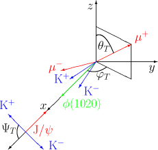
Figure 1: Decay angles in $B^{0}_{s}\rightarrow{J/\psi}\phi$.

The interference phase in the standard model is predicted to be $\phi_{s}\simeq-2\beta_{s}$, where $\beta_{s}=\mathrm{arg}(-(V_{ts}V_{tb}^{*})/(V_{cs}V_{cb}^{*}))$. The latest prediction [1] for $\beta_{s}$ is

$$2\beta_{s(\mathrm{SM})}=0.0363^{+0.0016}_{-0.0015}~{}\mathrm{rad}.$$

Very small deviations from the standard model expectation are also predicted by new physics models with minimal flavour violation, $|\phi_{s}|<0.05$, so that any observation of a large CP violation phase would rule out those models [2]. The analysis allows also a determination of the decay width difference, predicted by the standard model to be

$$\Delta\Gamma_{s(\mathrm{SM})}=0.087\pm 0.021~{}\mathrm{ps}^{-1},$$

but this quantity is expected having a reduced sensitivity to new physics processes [3].

2 Data samples and selections

The results obtained from the analysis of data collected in 2011 at $\sqrt{s}=7~{}\mathrm{TeV}$ by ATLAS, corresponding to an integrated luminosity ${\cal L}\sim 5~{}\mathrm{fb}^{-1}$, and in 2012 at $\sqrt{s}=8~{}\mathrm{TeV}$ by CMS, corresponding to an integrated luminosity ${\cal L}\sim 20~{}\mathrm{fb}^{-1}$, will be shown in the following.

Dedicated triggers have been developed for the analyses, requiring the presence of two muons forming a secondary vertex displaced from the primary interaction point, to achieve a sustainable trigger rate when collecting data at the very high luminosities provided by LHC. Events have been selected requiring two opposite charge muons and two other opposite charge tracks assumed to be kaons, forming a ${J/\psi}$ and a $\phi$ candidate respectively, with a common vertex.

3 Data analysis

The differential decay width is expressed as the sum of 10 functions of the time and the angles $\Theta=\theta_{T},\varphi_{T},\psi_{T}$, as defined in fig.1:

$$\frac{d^{4}\Gamma(B^{0}_{s}(t))}{d\Theta dt}=f(\Theta,\alpha,ct)\propto\sum_{i=1}^{10}O_{i}(\alpha,ct)\cdot g_{i}(\Theta)$$

$$\begin{array}[]{l}O_{i}(\alpha,ct)=N_{i}e^{-t/\tau}\left[a_{i}\cosh\left(\frac{1}{2}\Delta\Gamma_{s}ct\right)+b_{i}\sinh\left(\frac{1}{2}\Delta\Gamma_{s}ct\right)\right.\\ \rule{97.0pt}{0.0pt}\pm\left.c_{i}\cos\left(\Delta m_{s}ct\right)\pm d_{i}\sin\left(\Delta m_{s}ct\right)\makebox[0.0pt][l]{\rule{0.0pt}{0.0pt}}\right]\end{array}$$

$i$	$g_{i}(\theta_{T},\varphi_{T},\psi_{T})$	$N_{i}$	$a_{i}$	$b_{i}$	$c_{i}$	$d_{i}$
1	$2\cos^{2}\psi_{T}(1-\sin^{2}\theta_{T}\cos^{2}\varphi_{T})$	$|A_{0}|^{2}$	$1$	$D$	$C$	$-S$
2	$\sin^{2}\psi_{T}(1-\sin^{2}\theta_{T}\sin^{2}\varphi_{T})$	$|A_{\|}|^{2}$	$1$	$D$	$C$	$-S$
3	$\sin^{2}\psi_{T}\sin^{2}\theta_{T}$	$|A_{\bot}|^{2}$	$1$	$-D$	$C$	$S$
4	$-\sin^{2}\psi_{T}\sin 2\theta_{T}\sin\varphi_{T}$	$|A_{0}||A_{\bot}|$	$C\sin(\delta_{\bot}-\delta_{\|})$	$S\cos(\delta_{\bot}-\delta_{\|})$	$\sin(\delta_{\bot}-\delta_{\|})$	$D\cos(\delta_{\bot}-\delta_{\|})$
5	$\frac{1}{\sqrt{2}}\sin 2\psi_{T}\sin^{2}\theta_{T}\sin 2\varphi_{T}$	$|A_{0}||A_{\|}|$	$\cos(\delta_{\|}-\delta_{0})$	$D\cos(\delta_{\|}-\delta_{0})$	$C\cos(\delta_{\|}-\delta_{0})$	$-S\cos(\delta_{\|}-\delta_{0})$
6	$\frac{1}{\sqrt{2}}\sin 2\psi_{T}\sin 2\theta_{T}\sin\varphi_{T}$	$|A_{0}||A_{\bot}|$	$C\sin(\delta_{\bot}-\delta_{0})$	$S\cos(\delta_{\bot}-\delta_{0})$	$\sin(\delta_{\bot}-\delta_{0})$	$D\cos(\delta_{\bot}-\delta_{0})$
7	$\frac{2}{3}(1-\sin^{2}\theta_{T}\cos^{2}\varphi_{T})$	$|A_{S}|^{2}$	$1$	$-D$	$C$	$S$
8	$\frac{1}{3}\sqrt{6}\sin\psi_{T}\sin^{2}\theta_{T}\sin 2\varphi_{T}$	$|A_{S}||A_{\|}|$	$C\cos(\delta_{\|}-\delta_{S})$	$S\sin(\delta_{\|}-\delta_{S})$	$\cos(\delta_{\|}-\delta_{S})$	$D\sin(\delta_{\|}-\delta_{S})$
9	$\frac{1}{3}\sqrt{6}\sin\psi_{T}\sin 2\theta_{T}\cos\varphi_{T}$	$|A_{S}||A_{\bot}|$	$\sin(\delta_{\bot}-\delta_{S})$	$-D\sin(\delta_{\bot}-\delta_{S})$	$C\sin(\delta_{\bot}-\delta_{S})$	$S\sin(\delta_{\bot}-\delta_{S})$
10	$\frac{4}{3}\sqrt{3}(1-\sin^{2}\theta_{T}\cos^{2}\varphi_{T})$	$|A_{S}||A_{0}|$	$C\cos(\delta_{0}-\delta_{S})$	$S\sin(\delta_{0}-\delta_{S})$	$\cos(\delta_{0}-\delta_{S})$	$D\sin(\delta_{0}-\delta_{S})$

$$C=\frac{1-|\lambda|^{2}}{1+|\lambda|^{2}}\rule{28.45274pt}{0.0pt}S=-\frac{2|\lambda|\sin\phi_{s}}{1+|\lambda|^{2}}\rule{28.45274pt}{0.0pt}D=-\frac{2|\lambda|\cos\phi_{s}}{1+|\lambda|^{2}}.$$

The amplitudes $A_{\bot}$, $A_{0}$, $A_{\|}$, $A_{S}$ correspond to the $P$-wave and $S$-wave components, with their phases $\delta_{\bot}$, $\delta_{0}$, $\delta_{\|}$, $\delta_{S}$; $|\lambda|$ describes the direct CP violation. In the expression the signs of $c_{i}$ and $d_{i}$ coefficients are positive or negative for the decay of an initial $B^{0}_{s}$ or $\overline{B}^{0}_{s}$ respectively.

The differential width depends only on the differences among the phases $\delta$, so in the fit $\delta_{0}=0$ was assumed, and the difference $\delta_{S\bot}$ between $\delta_{\bot}$ and $\delta_{S}$ was fitted as an unique variable to reduce the correlation among the parameters. No direct violation was assumed in the measurement, therefore $|\lambda|=1$ was fixed.

The discrimination between the positive or negative initial flavour is obtained looking for a second $B$ produced in the event and inferring its flavour looking at the charge of its decay products; of course the charge-flavour correlation is diluted due to the presence of cascade decays and oscillations of the other $b$ hadron itself.

In ATLAS analysis [4] of $\sqrt{s}=7~{}\mathrm{TeV}$ data the flavour was tagged looking at the charge of particles contained in a cone around a muon, assumed to come from the semileptonic decay of a $b$; muons were classified according to their reconstruction class, combined or segment; if no muon was found the particles in a $b$-tagged jets were used. A “cone charge” was defined as

$$Q=\frac{\sum_{i}^{N_{\mathrm{tracks}}}q^{i}\cdot(p_{T,i})^{j}}{\sum_{i}^{N_{\mathrm{tracks}}}(p_{T,i})^{j}}$$

where $j=1.1$ and the sum was performed over the reconstructed tracks within a cone size of $\Delta R=0.5$. Charge distributions for $B^{+}$ and $B^{-}$ are shown in fig.2 and tagging performances are summarized in tab.1

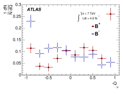
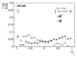
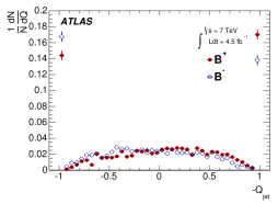
Figure 2: Opposite-side charge for $B^{+}$ and $B^{-}$, for segmented muons (left), combined muons (middle) and jets (right) in ATLAS analysis.

In CMS analysis [5] of $\sqrt{s}=8~{}\mathrm{TeV}$ data only semileptonic decays were used to tag the flavour, looking to both electrons and muons; in fig.3 the mistag fraction versus transverse momentum is shown.

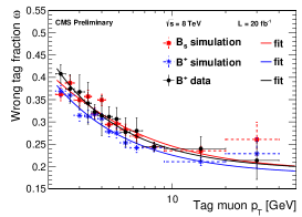
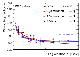
Figure 3: Mistag fraction versus transverse momentum for muons (left) and electrons (right) in CMS analysis.

The performance of the methods were measured with events containing the self-tagging decay $B^{+}\rightarrow{J/\psi}K^{+}$. The efficiency and tagging power of the algorithms are reported in tab.1 for ATLAS and tab.2 for CMS.

	Muons (c)	Muons (s)	$b$-jet
Efficiency [%]	$3.37\pm 0.04$	$1.08\pm 0.02$	$27.7\pm 0.1$
Dilution [%]	$50.6\pm 0.5$	$36.7\pm 0.7$	$12.68\pm 0.06$
Tagging power [%]	$0.86\pm 0.04$	$0.15\pm 0.02$	$0.45\pm 0.03$

Table 1: Performance of flavour tagging algorithm in ATLAS analysis; errors are statistical only.

	Muons	Electrons
Efficiency [%]	$4.55\pm 0.03\pm 0.08$	$3.26\pm 0.02\pm 0.01$
Mistag fraction [%]	$30.7\pm 0.4\pm 0.7$	$34.8\pm 0.3\pm 1.0$
Tagging power [%]	$0.68\pm 0.03\pm 0.05$	$0.30\pm 0.02\pm 0.04$

Table 2: Performance of flavour tagging algorithm in CMS analysis; errors are statistical only.

Efficiency and background have been estimated using simulation; background is made essentially by decay of other $B$ hadrons as $B^{0}_{d}$ , $B^{+}$ , $\Lambda_{b}$ and $B_{c}$. Efficiency have been estimated comparing the fully simulated signal sample, including detector response, with generator level information and computing the efficiency as a function of the three angles.

An unbinned maximum likelihood fit has been performed, including per-event resolution and tagging probability terms. The likelihood function is a sum of signal and background terms, with model functions for the three angles and the invariant mass, decay time and tagging information. The fitted distributions of invariant mass and proper time, or length, are shown in fig.4 for ATLAS and .fig.5 for CMS.

 

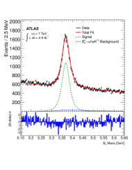
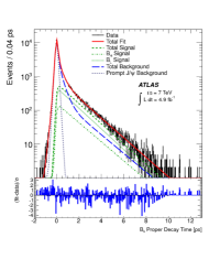
Figure 4: Invariant mass (left) and proper decay length (right) distributions in ATLAS fit.

 

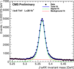
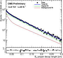
Figure 5: Invariant mass (left) and proper decay time (right) distributions in CMS fit.

Systematic uncertainties arise from efficiency and background estimation, from resolution and model functions. Potential biases have been estimated by pseudo-esperiments and included in the systematic error.

4 Results and expectations

The results of the fit are shown in tab.3 and fig.6; both experiments found a result in agreement with the prediction, but a significant test will require a smaller uncertainty, so further investigations are required.

	ATLAS	CMS
$\phi_{s}[\mathrm{rad}]$	$0.12\pm 0.25\pm 0.05$	$-0.03\pm 0.11\pm 0.03$
$\Delta\Gamma_{s}[\mathrm{ps}^{-1}]$	$0.053\pm 0.021\pm 0.010$	$0.096\pm 0.014\pm 0.007$

Table 3: Final results of CP violating phase and decay width difference measurements.

 

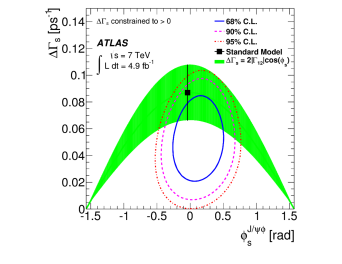
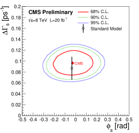
Figure 6: Likelihood contours in the $\phi_{s}-\Delta\Gamma_{s}$ plane in ATLAS (left) and CMS (right) measurements.

ATLAS made a study to estimate the measurement potential with new runs; more data will be available with the new run and increased luminosity, but this will correspond to a more difficult environment. ATLAS will have an improved pixel tracker, with a fourth layer, for Run2, and a new tracker with reduced pixel size for HL-LHC. The need to stay inside a necessarily limited trigger bandwidth will require harder cuts on muon $p_{T}$; two possible cuts have been considered, at $6~{}\mathrm{GeV}$ for Phase-1 and $11~{}\mathrm{GeV}$ for Phase-2 [6]. The upgraded tracker will allow a better vertex reconstruction and an improvement of 30% in proper decay time resolution, as shown in fig.7 (left). In principle this could be affected by the higher pileup, but a dedicated study showed that even in the hypothesis that the number of interaction could reach $N=200$, no significant effect appears visible, as shown in fig.7 (right).

 

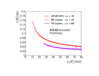
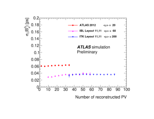
Figure 7: Proper decay time resolution in ATLAS against the $B^{0}_{s}$ transverse momentum (left) and the number of reconstructed primary vertices (right) in simulated $B^{0}_{s}\rightarrow{J/\psi}\phi$ events.

Estimating the signal yields applying the harder muon $p_{T}$ cuts to 2012 data and rescaling with efficiencies and luminosities the results shown in tab.4 are obtained.

${\cal L}(\mathrm{fb}^{-1})$	$p_{T\mu}$ cut $[\mathrm{GeV}]$	$\sigma(\phi_{s})$(stat)$[\mathrm{rad}]$
100	6	0.054
100	11	0.10
250	11	0.064
3000	11	0.022

Table 4: Estimated ATLAS statistical precisions of $\phi_{s}$ measurement for considered LHC periods.

5 Conclusions

The measurement of the CP violating phase $\phi_{s}$ can give hints or constraints of new physics beyond the standard model.

ATLAS and CMS performed a measurement by mean of an angular analysis of the decay $B^{0}_{s}\rightarrow{J/\psi}\phi$ using an initial flavour tagging to increase sensitivity. Results are compatible with previous result and SM expectations, but the uncertainty is currently much bigger than the theoretical error. More stringent tests will be obtained with more precise measurement to be done in the future LHC runs.

References

- [1] J.Charles et al., Predictions of selected flavor observables within the standard model, Phys. Rev. D 84, 033005 (2011). doi: 10.1103/PhysRevD.84.033005
- [2] G.Isidori, Flavor physics and CP violation, arXiv:1302.0661. url: http://arxiv.org/pdf/1302.0661v1.pdf
- [3] A.Lenz and U.Nierste, Numerical updates of lifetimes and mixing parameters of B mesons, arXiv:1102.4274. url: http://arxiv.org/pdf/1102.4274v1.pdf
- [4] ATLAS Collaboration, Flavor tagged time-dependent angular analysis of the decay and extraction of and the weak phase in ATLAS, Phys. Rev. D 90, 052007 (2014). doi: 10.1103/PhysRevD.90.052007
- [5] CMS Collaboration, Measurement of the CP-violating weak phase and the decay width difference using the decay channel, CMS-PAS-BPH-13-012. url: http://cds.cern.ch/record/1744869/files/BPH-13-012-pas.pdf
- [6] ATLAS Collaboration, ATLAS B-physics studies at increased LHC luminosity, potential for CP-violation measurement in the decay, ATL-PHYS-PUB-2013-010. url: http://cds.cern.ch/record/1604429/files/ATL-PHYS-PUB-2013-010.pdf