Data-based stochastic model reduction for the Kuramoto–Sivashinsky equation

Abstract

The problem of constructing data-based, predictive, reduced models for the Kuramoto-Sivashinsky equation is considered, under circumstances where one has observation data only for a small subset of the dynamical variables. Accurate prediction is achieved by developing a discrete-time stochastic reduced system, based on a NARMAX (Nonlinear Autoregressive Moving Average with eXogenous input) representation. The practical issue, with the NARMAX representation as with any other, is to identify an efficient structure, i.e., one with a small number of terms and coefficients. This is accomplished here by estimating coefficients for an approximate inertial form. The broader significance of the results is discussed.

Keywords: stochastic parametrization; NARMAX; Kuramoto-Sivashinsky equation; approximate inertial manifold.

1 Introduction

There are many high-dimensional dynamical systems in science and engineering that are too complex or computationally expensive to solve in full, and where only a relatively small subset of the degrees of freedom are observable and of direct interest. Under these conditions, it is useful to derive low-dimensional models that can predict the evolution of the variables of interest without reference to the remaining degrees of freedom, and reproduce their statistics at an acceptable cost.

We assume here that the variables of interest have been observed in the past, and we consider the problem of deriving low-dimensional models on the basis of such prior observations. We do the analysis in the case of the Kuramoto–Sivashinsky equation (KSE):

$$\frac{\partial v}{\partial t}+v\frac{\partial v}{\partial x}+\frac{\partial^{2}v}{\partial x^{2}}+\frac{\partial^{4}v}{\partial x^{4}}=0\,,x\in\mathbb{R},t>0;$$ (1)

$$v(x,t)=v(x+L,t);\,\,\,v(x,0)=v_{0}(x),$$

where $t$ is time, $x$ is space, $v$ is the solution of the equation, $L$ is an assumed spatial period, and $v_{0}$ is the initial datum. We pick a small integer $K$, and assume that one can observe only the Fourier modes of the solution with wave numbers $k=1,\dots K$ at a discrete sequence of points in time. To model the usual situation where the observed modes are not sufficient to determine a solution of the differential equations without additional input, we pick $K$ small enough so that the dynamics of a Galerkin-Fourier representation of the solution, truncated so that it contains only $K$ modes, are far from the dynamics of the full system. The goal is to account for the effects of “model error”, i.e. for the effects of the missing “unresolved” modes on the “resolved” modes, by suitable terms in reduced equations for the resolved modes, using the information contained in the observations of the resolved modes; we are not interested in the unresolved modes per se. In the present paper the observations are obtained by a solution of the full system; we hope that our methods are applicable to problems where the data come from physical measurements, including problems where a full model is not known.

We start from the truncated equations for the resolved modes, and solve an inverse problem where the data are used to estimate the effects of model error, i.e., what needs to be added to the truncated equations for the solution of the truncated equations to agree with the data. Once these effects are estimated, they need to be identified, i.e., summarized by expressions that can be readily used in computation. In our problem the added terms can take a range of values for each value of the resolved variables, and therefore a stochastic model is a better choice than a deterministic model. We solve the inverse problem within a discrete-time setting (see [9]), and then identify the needed terms within a NARMAX (Nonlinear Autoregression with Moving Average and eXogenous input) representation of discrete time series. The determination of missing terms from data is often called a “parametrization”; what we are presenting is a discrete stochastic parametrization. The main difficulty in stochastic parametrization, as in non-parametric statistical inference problems, is making the identified representation efficient, i.e., with a small number of terms and coefficients. We accomplish this by a semi-parametric approach: we propose terms for the NARMAX representation from an approximate “inertial form” [25], i.e., a system of ordinary differential equations that describes the motion of the system on a finite-dimensional, globally attracting manifold called an “inertial manifold”. (Relevant facts from inertial manifold theory are reviewed later.)

A number of stochastic parametrization methods have been proposed in recent years, often in the context of weather and climate prediction. In [35, 47, 1], model error is represented as the sum of an approximating polynomial in the resolved variables, obtained by regression, and a one-step autoregression. The shortcomings of this representation as a general tool are that it does not allow the model error to depend sufficiently on the past values of the solution, that the model error is calculated inaccurately, especially when the data are sparse, and that the autoregression term is not necessarily small, making it difficult to solve the resulting stochastic equations accurately. Detailed comparisons between this approach and a discrete-time NARMAX approach can be found in [9]. In [12, 31] the model error is represented as a conditional Markov chain that depends on both current and past values of the solution; the Markov chain is deduced from data by binning and counting, assuming that exact observations of the model error are available, i.e., that the inverse problem has been solved perfectly. It should be noted that the Markov chain representation is intrinsically discrete, making this work close to ours in spirit. In [32] the noise is treated as continuous and represented by a hypo-elliptic system that is partly analogous to the NARMAX representation, once translated from the continuum to the grid. An earlier construction of a reduced approximation can be found in [7], where the approach was not yet fully discrete. Other interesting related work can be found in [5, 15, 14, 23, 30]. The present authors’ previous work on the discrete-time approach to stochastic parametrization and the use of NARMAX representations can be found in [9].

The KSE is a prototypical model of spatiotemporal chaos. As a nonlinear PDE, it has features found in more complex models of continuum mechanics, yet its analysis and numerical solution are fairly well understood because of its relatively simple structure. There is a lot of previous work on stochastic model reduction for the KSE. Yakhot[48] developed a dynamic renormalization group method for reducing the KSE, and showed that the model error generates a random force and a positive viscosity. Recent development of this method can be found in [41, 42]. Toh [46] studied the statistical properties of the KSE, and constructed a statistical model to reproduce the energy spectrum. Rost and Krug [39] presented a model of interacting particles on the line which exhibits spatiotemporal chaos, and made a connection with the stochastic Burgers equation and the KPZ equation.

Stinis [43] addressed the problem of reducing the KSE as an under-resolved computation problem with missing initial data, and used the Mori-Zwanzig (MZ) formalism [50] in the finite memory approximation [8, 6] to produce a reduced system that can make short-time predictions. Full-system solutions were used to compute the conditional means used in the reduced system. As discussed in [9], the NARMAX representation can be thought of as both a generalization and an implementation of the MZ formalism, and the full-system solutions used by Stinis can be viewed as data, so that the pioneering work of Stinis is close in spirit to our work. We provide below a comparison of our work with that of Stinis.

The paper is organized as follows. In section 2, we introduce the Kuramoto–Sivashinsky equation, the dynamics of its solutions, and its numerical solution by spectral methods. In section 3 we apply the discrete approach for the determination of reduced systems to the KSE, and discuss the NARMAX representation of time series. In section 4 we use an inertial form to determine the structure of a NARMAX representation for the KSE, and estimate its coefficients. Numerical results are presented in section 5. Conclusions and the broader significance of the work, as well as its limitations, are discussed in a concluding section.

2 The Kuramoto-Sivashinsky equation

We begin with basic observations: in Eq. (1), the term ${\partial^{2}v}/{\partial x^{2}}$ is responsible for instability at large scales, the dissipative term ${\partial^{4}v}/{\partial x^{4}}$ provides damping at small scales, and the non-linear term $v{\partial v}/{\partial x}$ stabilizes the system by transferring energy between large and small scales. To see this, first write the KSE in terms of Fourier modes:

$$\frac{d}{dt}v_{k}=(q_{k}^{2}-q_{k}^{4})v_{k}-\frac{iq_{k}}{2}\sum_{l=-\infty}^{\infty}v_{l}v_{k-l},$$ (2)

where the $v_{k}(t)$ are the Fourier coefficients

$$v_{k}(t)~{}:=~{}\mathcal{F}[v(\cdot,t)]_{k}~{}:=~{}\frac{1}{L}\int_{0}^{L}v(x,t)e^{-iq_{k}x}dx,$$ (3)

where $q_{k}=\frac{2\pi k}{L}$, $k\in{\mathbb{Z}}$, and ${\mathcal{F}}$ denotes the Fourier transform, so that

$$v(x,t)=\mathcal{F}^{-1}[v_{\cdot}(t)]=\sum_{k=-\infty}^{+\infty}v_{k}(t)e^{iq_{k}x}.$$ (4)

Since $v$ is real, the Fourier modes satisfy $v_{-k}=v_{k}^{\ast}$, where $v_{k}^{\ast}$ is the complex conjugate of $v_{k}$. We refer to $|v_{k}(t)|^{2}$ as the “energy” of the $k$th mode at time $t$.

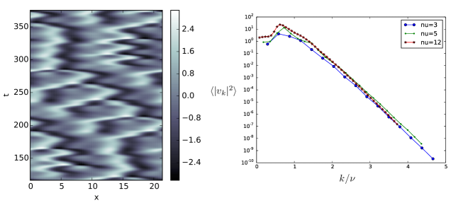
Figure 1: Solutions of the KSE. Left: a sample solution of the KSE. Right: Mean energy $\langle|v_{k}|^{2}\rangle$ as a function of $k/\nu$, where $\nu=L/2\pi$ is the number of unstable modes, for a number of different values of $L$.

Next, we consider the linearization of the KSE about the zero solution. In the linearized equations, the Fourier modes are uncoupled, each represented by a first-order scalar ODE with eigenvalue $q_{k}^{2}-q_{k}^{4}$. Modes with $|q_{k}|>1$ are linearly stable; modes with $|q_{k}|\leq 1$ are not. The linearly unstable modes, of which there are $\nu={\lfloor{L/2\pi}\rfloor}$, are coupled to each other and to the damped modes through the nonlinear term. Observe that if the nonlinear terms were not present, most initial conditions would lead to solutions whose energies blow up exponentially in time. The KSE is, however, well-posed (see, e.g., [10]), and it can be shown that solutions remain globally bounded in time (in suitable function spaces) [19, 4]. The solutions of Eq. (1) do not grow exponentially because the quadratic nonlinearities, which formally conserve the $L^{2}$ norm, serve to transport energy from low to high modes. Figure 1 shows an example solution, as well as the energy spectrum $\langle|v_{k}|^{2}\rangle,$ where $\langle\phi\rangle$ denotes the limit of $\frac{1}{T}\int_{0}^{T}\phi(v(t))dt$ as $T\to\infty~{}.$ The energy spectrum has a characteristic “plateau” for small wave numbers, which gives way to rapid, exponential decay as $k$ increases, see Figure 1(right). This concentration of energy in the low-wavenumber modes is reflected in the cellular character of the solution in Figure 1(left), where the length scale of the cells is determined by the modes carrying the most energy.

Another feature of the nonlinear energy transfer is that the KSE possesses an inertial manifold $M$. When the KSE is viewed as an infinite-dimensional dynamical system on a suitable function space $B$, there exists a finite-dimensional submanifold $M\subset B$ such that all solutions of the KSE tend asymptotically to $M$ (see e.g. [10]). The long-time dynamics of the KSE are thus essentially finite-dimensional. Moreover, it can be shown that for sufficiently large $N$ ($N>\mbox{dim}(M)$ at the very minimum), an inertial manifold $M$ can be written in the form

$$M=\{x+\psi(x)|x\in\pi_{N}(B)\}$$ (5)

where $\pi_{N}$ is the projection onto the span of $\{e^{ikx},k=1,\cdots,N\}$, and $\psi:\pi_{N}(B)\to(\pi_{N}(B))^{\perp}$ is a Lipschitz-continuous map. That is to say, for trajectories lying on the inertial manifold $M$, the high-wavenumber modes are completely determined by the low-wavenumber modes. Inertial manifolds will be useful in Section 4, and we say more about them there.

The KSE system is Galilean invariant; if $v(x,t)$ is a solution, then $v(x-ct,t)+c$, with $c$ an arbitrary constant velocity, is also a solution. Without loss of generality, we set $\int v(x,0)dx=0$, which implies that $v_{0}(0)=0$. From (2), we see that $v_{0}(t)\equiv 0$ for all $t$ and $\int v(x,t)dx\equiv 0$. In physical terms, solutions $v(x,t)$ of the KSE can be interpreted as the velocity of a propagating “front,” for example as in flame propagation, and this decoupling of the $v_{0}$ equation from $v_{k}$ for $k\neq 0$ means the mean velocity is conserved.

Chaotic dynamics and statistical assumptions. Numerous studies have shown that the KSE exhibits chaotic dynamics, as characterized by a positive Lyapunov exponent, exponentially decaying time correlations, and other signatures of chaos (see, e.g., [24] and references therein). Roughly speaking, this means that nearby trajectories tend to separate exponentially fast in time, and that, though the KSE is a deterministic equation, its solutions are unpredictable in the long run as small errors in initial conditions are amplified. Chaos also means that a statistical modeling approach is natural. In what follows, we assume our system is in a chaotic regime, characterized by a translation-invariant physical invariant probability measure (see, e.g., [16, 49] for the notion of physical invariant measures and their connections to chaotic dynamics). That is, we assume that numerical solutions of the KSE, sampled at regular space and time intervals, form (modulo transients) multidimensional time series that are stationary in time and homogeneous in space, and that the resulting statistics are insensitive to the exact choice of initial conditions. Except where noted, this assumption is consistent with numerical observations. Hereafter we will refer to this as “the” ergodicity assumption, as this is the assumption of ergodicity needed in the present paper.

The translation-invariance part of our ergodicity assumption has the consequence, the Fourier coefficients cannot have a preferred phase in steady state, i.e., the physical invariant measure has the property that if we write the $k$th Fourier coefficient $v_{k}$ (see below) as $a_{k}e^{i\theta_{k}}$, then the $\theta_{k}$ are uniformly distributed. The theory of stationary stochastic processes also tells us that distinct Fourier modes are uncorrelated [6], though they are generally not independent: one can readily show this by, e.g., checking that ${\rm cov}(|v_{k}|^{2},|v_{\ell}|^{2})\neq 0$ numerically. (Such energy correlations are yet another consequence of the nonlinear term acting to transfer energy between modes.)

Numerical solution. For purposes of numerical approximation, the system can be truncated as follows: the function $v(x,t)$ is sampled at the grid points $x_{n}=nL/N,n=0,\dots,N-1$, so that $v^{N}=\left(v(x_{0},t),\dots,v(x_{N-1},t)\right)$, where the superscript $N$ in $v^{N}$ is a reminder that the sampled $v$ varies as $N$ changes. The Fourier transform $\mathcal{F}$ is replaced by the discrete Fourier transform ${\mathcal{F}}_{N}$ (assuming $N$ is even):

$$v_{k}^{N}={\mathcal{F}}_{N}[v(\cdot,t)]_{k}=\sum_{n=0}^{N-1}v^{N}(x_{n},t)e^{-iq_{k}x_{n}},\,$$

and

$$\,v^{N}(x_{n},t)={\mathcal{F}}_{N}^{-1}[v_{\cdot}^{N}(t)]=\frac{1}{N}\sum_{k=-N/2+1}^{N/2}v_{k}^{N}(t)e^{iq_{k}x_{n}}.$$

Noting that $\hat{v}_{0}^{N}=0$ due to Galilean invariance, and setting $\hat{v}_{N/2}^{N}=0$, we obtain a truncated system

$$\frac{d}{dt}v_{k}^{N}=(q_{k}^{2}-q_{k}^{4})v_{k}^{N}-\frac{iq_{k}}{2}\sum_{\begin{subarray}{c}1\leq|l|\leq N,\\ 1\leq\left|k-l\right|\leq N\end{subarray}}v_{l}^{N}v_{k-l}^{N},~{}$$ (6)

with $k=-N/2+1,\dots,N/2$. This is a system of ODE (of the real and imaginary parts of $v_{k}^{N}$) in $\mathbb{R}^{N-2}$, since $v_{-k}^{N}=v_{k}^{N,\ast}$ and $v_{N/2}^{N}=$ $v_{0}^{N}\equiv 0$.

Fourier modes with large wave numbers are typically small and can be neglected, as can be seen from a linear analysis: $v_{k}$ decreases at approximately the rate $e^{(q_{k}^{2}-q_{k}^{4})t}$, where $q_{k}={kL}/{2\pi}$ (see Figure 1(right)). A truncation with $N\geq 8\nu=8{\lfloor{L/2\pi}\rfloor}$ can be considered accurate. In the following, a truncated system with $N=32\nu=32{\lfloor{L/2\pi}\rfloor}$ is considered to be the “full” system, and we aim to construct reduced models for $K<2\nu\approx L/\pi$. Except when $N$ is small, the system (6) is stiff (since $q_{k}$ grows rapidly with $k$). To handle this stiffness and maintain reasonable accuracy, we generate data by solving the truncated KSE by an exponential time difference fourth order Runge-Kutta method (ETDRK4) [11, 28] with standard $3/2$ de-aliasing (see, e.g., [34, 20]). We solve the full system with a small step size $dt$, and then make observations of the modes with wave numbers $k=1,\dots,K$ at a times separated by a larger time interval $\delta>dt$, and denote the observed data by

$$\left\{v_{k}(t_{n}),k=1,\dots,K,n=0,\dots,T\right\},$$

where $t_{n}=n\delta$.

To predict the evolution of $K$ observed modes with wave numbers $k=1,\dots,K$, it is natural to start from the truncated system that includes only these modes, i.e., the system (6) with $N=2(K+1)$. However, when one takes $K$ to be relatively small (as we do in the present paper), large truncation errors are present, and the dynamics of the truncated system are very different from those of the full system.

3 A discrete-time approach to stochastic parametrization and the NARMAX representation

Suppose one is given a dynamical system

$$\frac{d\phi}{dt}=F(\phi)$$ (7)

where the variables are partitioned as $\phi=(u,w)$, with $u$ representing a (possibly quite small) subset of variables of direct interest. The problem of model reduction is to develop a reduced dynamical system for predicting the evolution of $u$ alone. That is, one wishes to find an equation for $u$ that has the form

$$\frac{du}{dt}=R({u})+z(t),$$ (8)

where $R(u)$ is a function of $u$ only, and $z(t)$ represents the model error, i.e., the quantity one should add to $R(u)$ to obtain the correct evolution. For example, if $\phi$ represents the full state $(v_{k},k\in\mathbb{Z})$ of a KSE solution and $u$ represents the low-wavenumber modes $(v_{-K},v_{-K+1},\cdots,v_{K})$, then $R$ can correspond to a $K$-mode truncation of the KSE. In general, the model error $z$ must depend on $u$, since the resolved variables $u$ and unresolved variables $w$ typically interact.

The usual approach to stochastic parametrization and model reduction as formulated above is to identify $z$ as a stochastic process in the differential equation (8) from data (see [35, 47, 12, 32] and references therein). This approach has major difficulties. First, it leads to the challenging problem of statistical inference for a continuous-time nonlinear stochastic system from partial discrete observations [36, 40]. The data are measurements of $u$, not of $z$; to find values of $z$ one has to use equation (8) and differentiate $x$ numerically, which may be inaccurate because $z$ may have high-frequency components or fail to be sufficiently smooth, and because the data may not be available at sufficiently small time intervals. Then, if one can successfully estimate values of $z$ and then identify it, equation (8) becomes a nonlinear stochastic differential system, which may be hard to solve with sufficient accuracy (see e.g [29, 33]).

To avoid these difficulties, a purely discrete-time approach to stochastic parametrization was proposed in [9]. This approach avoids the difficult detour through a continuous-time stochastic system followed by its discretization, by working entirely in a discrete-time setting. It starts from the truncated equation

$$\frac{dy}{dt}=R({y}).$$

($y$ differs from $u$ in that its evolution equation is missing the information represented by the model error $z(t)$ in Eq. (8), and so is not up to the task of computing $u$.) Fix a step size $\delta>0$, and choose a method of time-discretization, for example fourth-order Runge-Kutta. Then discretize the truncated equation above to obtain a discrete-time approximation of the form

$$y^{n+1}=y^{n}+\delta R^{\delta}(y^{n}).$$

(The function $R^{\delta}$ depends on the numerical time-stepping scheme used.) To estimate the model error, write a discrete analog of equation (8):

$$u^{n+1}=u^{n}+\delta R^{\delta}(u^{n})+\delta z^{n+1}.$$ (9)

Note that a sequence of values of $z^{n+1}$ can be computed from data using

$$z^{n+1}=\frac{u^{n+1}-u^{n}}{\delta}-R^{\delta}(u^{n}),$$ (10)

where the values of $u$ are the observed values; the resulting values of $z$ account for both the model error in (8) and the numerical error in the discretization $R^{\delta}(u^{n})$. The task at hand is to identify the time series $\left\{z^{n}\right\}$ as a discrete stochastic process which depends on $u$. Once this is done, equation (9) will be used to predict the evolution of $u$. There is no need to approximate or differentiate, and there is no stochastic differential equations to solve. Note that the $z^{n}$ depend on the numerical error as well as on the model error, and may not be good representations of the continuum model error; we are not interested in the latter, we are only interested in modeling the solution $u$.

The sequence $\left\{z^{n}\right\}$ is a stationary time series, which we represent via a NARMAX representation, with $u$ as an exogenous input. This representation makes it possible to take into account efficiently the non-Markovian features of the reduced system as well as model and numerical errors. The NARMAX representation is versatile, easy to implement and reliable. The model inferred from data is exactly the same as the one used for prediction, which is not the case for a continuous-time system because of numerical approximations. The disadvantage of the discrete approach is that the discrete system depends on both the spacing of the observed data and the method of time-discretization, so that data sets with different spacing lead to different discrete systems.

The NARMAX representation has the form:

$$u^{n+1} = u^{n}+\delta R^{\delta}(u^{n})+\delta z^{n+1},$$

$$z^{n} = \Phi^{n}+\xi^{n},$$ (11)

for $n=1,2,\dots$, where $\left\{\xi^{n}\right\}$ is a sequence of independent identically distributed random variables, the first equation repeats equation (9), and $\Phi^{n}$ is a functional of current and past values of $\left(u,z,\xi\right)$, of the parametrized form:

$$\Phi^{n}=\mu+\sum_{j=1}^{p}A_{j}z^{n-j}+\sum_{j=1}^{r}B_{j}Q_{j}({u}^{n-j})+\sum_{j=1}^{q}C_{j}\xi^{n-j},$$ (12)

where $\left(Q_{j},\ i=1,\dots,r\right)$ are functions to be chosen appropriately and $\left(\mu,A_{j},B_{j},C_{j}\right)$ are constant parameters to be inferred from data. Here we assume that the real and complex parts of $\xi^{n}$ are independent and have Gaussian distributions with mean zero and diagonal covariance matrix $\sigma^{2}$.

We call the above equations a NARMAX representation because the time series $\{z^{n}\}$ in equations (11)–(12) resemble the nonlinear autoregression moving average with exogenous input (NARMAX) model in e.g., [2, 22, 17]. In (12), the terms in $z$ are the autoregression part of order $p$, the terms in $\xi$ are the moving average part of order $q$, and the terms $Q_{j}$ which depend on $u$ are the exogenous input terms. One should note that our representation is not quite a NARMAX model in the usual sense, because the exogenous input in NARMAX is supposed to be independent of the output $z$, while here it is not. The system (11)–(12) is a nonlinear autoregression moving average (NARMA) representation of the time series $\left\{u^{n}\right\}$: by substituting (10) into (12) we obtain a closed system for $u:$

$$u^{n+1}=u^{n}+\delta R^{\delta}(u^{n})+\delta\Psi^{n}+\delta\xi^{n+1},$$ (13)

where $\Psi^{n}$ is a functional of the past values of $u$ and $\xi$.

The form of the system (11)–(12) is quite general. $\Phi^{n}$ can be a more general nonlinear functional of the past values of $\left(u,z,\xi\right)$ than the one in (12). The additive noise $\xi$ can be replaced by a multiplicative noise. We leave these further generalizations to future work. The main task in identification of a NARMAX representation is to determine the structure of the functional $\Phi^{n}$, that is, determine the terms that are needed, then determine the orders $(p,r,q)$ in (12) and estimate the parameters.

4 Determination of the NARMAX representation

To apply NARMAX to the KSE, one must first decide on the structure of the model for $z^{n}$. In particular, one must decide which nonlinear terms to include in the ansatz. We note that a priori, it is clear that some nonlinear terms are necessary, as a simple linear ansatz is very unlikely to be able to capture the dynamics of the KSE. This is because distinct modes are uncorrelated (see section 2), so that if the ansatz for $z^{n}$ contains only linear terms, then the different components of our stochastic model for $z^{n}$ would be independent, and one would not expect such a model to capture the energy balance between the unresolved modes (see e.g. [32]).

But the question remains: which nonlinear terms? One option is to include all nonlinear terms up to some order. This leads to a difficult parameter estimation problems because of the large numbers of parameters involved. Moreover, a model with many terms is likely to overfit, which complicates the model and leads to poor predictive performance (see e.g. [2]). What we do here instead is use inertial manifolds as a guide to selecting suitable nonlinear terms. We note that our construction satisfies the physical realizability constraints discussed in [32].

4.1 Approximate inertial manifolds

We begin with a quick review of approximate inertial manifolds, following [25]. Write the KSE (1) in the form

$$\frac{dv}{dt}=Av+f(v),\ \ v(x,0)=v_{0}\in H,$$

where the linear operator $A$ is the fourth derivative operator $-{\partial^{4}}/{\partial x^{4}}$ or, in Fourier variables, the infinite-dimensional diagonal matrix with entries $-q_{k}^{4}$ in (2), and where $f(v)=-v{\partial v}/{\partial x}-{\partial^{2}v}/{\partial x^{2}}$ or its spectral analog, and where $H=\left\{v\in L^{2}[0,L]|v(x)=v(x+L),x\in\mathbb{R}\right\}$. An inertial manifold is a positively-invariant finite-dimensional manifold that attracts all trajectories exponentially; see e.g. [10, 37] for its existence, and see e.g. [45, 27] for estimates of its dimension. It can be shown that inertial manifolds for the KSE are realizable as graphs of functions $\psi:PH\rightarrow QH$, where $P$ is a suitable finite-dimensional projection (see below), and $Q=I-P$. The inertial form (the ordinary differential equation that describes motion restricted to the inertial manifold) can be expressed in terms of the projected variable $u$ by

$$\frac{du}{dt}=PAu+Pf(u+\psi(u)),$$ (14)

where $u=Pv$. Different methods for the approximation of inertial manifolds have been proposed [25, 26, 38]. These methods approximate the function $w=\psi(u)$ by approximating the projected system on $QH$,

$$\frac{dw}{dt}=QAw+Qf(u+w),\ \ \ w(0)=Qv_{0}.$$ (15)

In practice, $P$ is typically taken to be the projection onto the span of the first $m$ eigenfunctions of $A$, for example, one can set $u=Pv=(v_{-m},v_{-m+1},\dots,v_{m})$, the first $2m$ Fourier modes. The dimension of the inertial manifold is generally not known a priori [27], so $m$ is usually taken to be a large integer. It is shown in [18] that for large enough $m$ and for $v=u+w$ on the inertial manifold, ${dw}/{dt}$ is relatively small. Neglecting ${dw}/{dt}$ in (15) we obtain an approximate equation for $w$:

$$w=-A^{-1}Qf(u+w).$$ (16)

Approximations of $\psi$ can then be obtained by setting up fixed point iterations,

$$\psi_{0}=0,\,\,\,\psi_{n+1}=-A^{-1}Qf(u+\psi_{n}).$$ (17)

and stopping at a particular finite value of $n$, which yields an “approximate inertial manifold” (AIM). The accuracy of AIM improves as its dimension $m$ increases, in the sense that the distance between the AIM and the global attractor of the KSE decreases at the rate $|q_{m}|^{-\gamma}$ for some $\gamma>0$ [25].

In the application to our reduced KSE equation, one may try to set $m=K$. However, our cutoff $K<2\nu\approx\frac{L}{\pi}$ is too small for there to be a well-defined inertial form, since this is relatively close to the number $\nu={\lfloor{L/2\pi}\rfloor}$ of linearly unstable modes, and we generally expect any inertial manifold to have dimension much large than $2\nu$. Nevertheless, we will see that the above procedure for constructing AIMs provides a useful guide for selecting nonlinear terms for NARMAX. This is unsurprising, since inertial manifolds arise from the nonlinear energy transfer between low and high modes and the strong dissipation at high modes, which is exactly what we hope to capture.

4.2 Structure selection

We now determine the structure of the NARMAX model, i.e., decide what terms should appear in (12). These terms should correctly reflect how $z$ depends on $u$ and $\xi$. Once the terms are determined, parameter estimation is relatively easy, as we see in the next subsection. The number of terms should be as small as possible, to save computing effort and to reduce the statistical error in the estimate of the coefficients. One could try to determine the terms to be kept by looking for the terms that contribute most to the output variance, see [2, Chapter 3] and the references there. This approach fails to identify the right terms for strongly nonlinear systems such as the one we have. Other ideas based on a purely statistical approach have been explored e.g. in [2, Chapter 9]. In the present paper, we design the nonlinear terms in (12) in the NARMAX model, which represents the model error in the $K$-mode truncation of the KSE, using the theory of inertial manifolds sketched above.

In our setting, $u=\left(v_{-K},\dots,v_{K}\right)$. Because of the quadratic nonlinearity, only the modes with wave number $|k|=K+1,K+2,\dots,2K$ interact directly with the observed modes in $u$; hence we set $w=\left(v_{-2K},\dots v_{-K-1},v_{K+1},\dots v_{2K}\right)$ in Eq. (16). Using the result of a one-step iteration $\psi_{1}=-A^{-1}Qf(u)$ in (17) we obtain an expression for the high mode $v_{k}$ as a function of the low modes $u$:

$$\psi_{1,k}=-\left(A^{-1}Qf(u)\right)_{k}=-\frac{i}{2}q_{k}^{-4}\sum_{1\leq|l|\leq K,1\leq\left|k-l\right|\leq K}v_{l}v_{k-l},$$

for $\left|k\right|=K+1,K+2,\dots,2K$.

Our goal is to approximate the model error of the $K$-mode Galerkin truncation, $Pf(u+\psi(u))-Pf(u)$, so that the reduced model is closer to the attractor than the Galerkin truncation. In standard approximate inertial manifold methods, the model error is approximated by $Pf(u+\psi_{1}(u))-Pf(u)$. Since $K$ is relatively small in our setting, we do not expect the AIM approximation to be effective. However, in stochastic parameterization, we only need a parametric representation of the model error, and more specifically, to derive the nonlinear terms in the NARMAX model. As the AIM procedure implicitly takes into account energy transfer between Fourier modes due to nonlinear interactions as well as the strong dissipation in high modes, it can be used to suggest nonlinear terms to include in our NARMAX model. That is, the above expressions of $\psi_{1}$, $Pf(u+\psi_{1}(u))-Pf(u)$ provide explicit nonlinear terms $\{\phi_{1,k}\phi_{1,l},\phi_{1,k}v_{j}\}$ we need (with $K<|k|,|l|\leq 2K,|j|\leq K$); we simply leave the coefficients of these terms as free parameters to be determined from data. Roughly speaking, the NARMAX can be viewed as a regression implementation of a parametric version of AIM.

Implementing the above observations in discrete time, we obtain the following terms to be used in the discrete reduced system:

$$\widetilde{u}_{j}^{n}=\left\{\begin{array}[]{ll}u_{j}^{n},&1\leq j\leq K;\\ i\sum_{l=j-K}^{K}u_{l}^{n}u_{j-l}^{n},&K<j\leq 2K.\end{array}\right.$$ (18)

The modes with negative wave numbers are defined by $\widetilde{u}_{-j}^{n}=\widetilde{u}_{j}^{n,\ast}$. This yields the discrete stochastic system

$$u_{k}^{n+1} = u_{k}^{n}+\delta R_{k}^{\delta}(u^{n})+\delta z_{k}^{n+1},$$

$$z_{k}^{n} = \Phi_{k}^{n}+\xi_{k}^{n},$$

where the functional $\Phi_{k}^{n}$ has the form:

$$\Phi_{k}^{n}(\theta_{k}) = \mu_{k}+\sum_{j=1}^{p}a_{k,j}z_{k}^{n-j}+\sum_{j=0}^{r}b_{k,j}u_{k}^{n-j}+\sum_{j=1}^{K}c_{k,j}\widetilde{u}_{j+K}^{n}\widetilde{u}_{j+K-k}^{n}$$ (19)

$$+c_{k,(K+1)}R_{k}^{\delta}(u^{n})+\sum_{j=1}^{q}d_{k,j}\xi_{k}^{n-j},$$

for $1\leq k\leq K$. Here $\theta_{k}=\left(\mu_{k},a_{k,j},b_{k,j},c_{k,j},d_{k,j}\right)$ are real parameters to be estimated from data. Note that each one of the random variables $\xi_{k}^{n}$ affects directly only one mode $u_{k}^{n}$, as is consistent with the vanishing of correlations between distinct Fourier modes (see section 2).

We set $\Phi_{-k}^{n}=\Phi_{k}^{n,\ast}$ so that the solution of the stochastic reduced system satisfies $u_{-j}^{n}=u_{j}^{n,\ast}$. We include the terms in $R^{\delta}_{k}(u^{n})$ because the way they were introduced in the above reduced stochastic system does not guarantee that they have the optimal coefficients for the representation of $z$; the inclusion of these terms in $\Phi^{n}_{k}$ makes it possible to optimize these coefficients. This is similar in spirit to the construction of consistent reduced models in [23], though simpler to implement.

4.3 Parameter estimation

We assume in this section that the terms and the orders $\left(p,r,q\right)$ in the NARMAX representation have been selected, and estimate the parameters as follows. To start, assume that the reduced system has dimension $K$, that is, the variables $u^{n}$, $z^{n}$, $\Phi^{n}$ and $\xi^{n}$ have $K$ components. Denote by $\theta_{k}=(\mu_{k},A_{k,j},B_{k,j},C_{k,j})$ the set of parameters in the $k$th component of $\Phi^{n}$, and $\theta=(\theta_{1},\theta_{2},\dots,\theta_{K})\,$. We write $\Phi_{k}^{n}$ as $\Phi_{k}^{n}(\theta_{k})$ to emphasize that $\Phi$ depends on $\theta_{k}$.

Recall that the real and complex parts of the components of $\xi^{n}$ are independent $N(0,\sigma_{k}^{2})$ random variables. Then, following (11), the log–likelihood of the observations $\left\{u^{n},q+1\leq n\leq N\right\}$ conditioned on $\{\xi^{1},\dots,\xi^{q}\}$ is (up to a constant)

$$l(\theta,\sigma^{2}|\xi^{1},\dots,\xi^{q})=-\sum_{k=1}^{K}\left(\sum_{n=q+1}^{N}\frac{\left|z_{k}^{n}-\Phi_{k}^{n}(\theta)\right|^{2}}{2\sigma_{k}^{2}}+(N-q)\ln\sigma_{k}^{2}\right).$$ (20)

If $q=0$, this is the standard likelihood of the data $\left\{u^{n},1\leq n\leq N\right\}$, and the values of $z^{n}$ and $\Phi^{n}(\theta)$ can be computed from the data $u^{n}$ using (10) and (19), respectively. However, if $q>0$, the sequence $\{\Phi_{k}^{n}(\theta)\}$ cannot be computed directly from data, due to its dependence on the noise sequence $\{\xi^{n}\}$, which is unknown. Note that once the values of $\{\xi^{1},\dots,\xi^{q}\}$ are available, one can compute recursively the sequence $\{\Phi_{k}^{n}(\theta)\}$ for $n\geq q+1$ from data. Hence we can compute the likelihood of $\left\{u^{n},q+1\leq n\leq N\right\}$ conditional on $\{\xi^{1},\dots,\xi^{q}\}$. If the stochastic reduced system is ergodic and the data come from this system, the MLE is asymptotically consistent (see e.g. [21, 22]), and hence the values of $\xi^{1},\dots,\xi^{q}$ do not affect the result if the data set is long enough. In practice, we can simply set $\xi^{1}=\dots=\xi^{q}=0$, the mean of these variables.

Taking partial derivatives with respect to $\sigma_{k}^{2}$ and noting that $\left|z_{k}^{n}-\Phi_{k}^{n}(\theta_{k})\right|$ is independent of $\sigma_{k}^{2}$, we find that the maximum likelihood estimators (MLE) $\hat{\theta},\hat{\sigma}^{2}$ satisfy the following equations:

$$\hat{\theta}_{k}=\arg\min_{\theta_{k}}S_{k}(\theta_{k}),~{}\hat{\sigma}_{k}^{2}=\frac{1}{2(N-q)}S(\hat{\theta}_{k}),$$ (21)

where

$$S_{k}(\theta_{k}):=\sum_{n=q+1}^{N}\left|z_{k}^{n}-\Phi_{k}^{n}(\theta_{k})\right|^{2}.$$

Note first that in the case $q=0$, the MLE $\hat{\theta}_{k}$ follows directly from least squares, because $\Phi_{k}^{n}$ is linear in the parameter $\theta_{k}$ and its terms can be computed from data. If $q>0$, the MLE $\hat{\theta}_{k}$ can be computed either by an optimization method (e.g. quasi-Newton method), or by iterative least squares method (see e.g. [13]). With either method, one first computes $\Phi_{k}^{n}(\theta_{k})$ with the current value of parameter $\theta_{k}$, and then one updates $\theta_{k}$ (by gradient search methods or by least squares), and repeats until the error tolerance for convergence is reached. The starting values of $\theta_{k}$ for the iterations for either method are set to be the least square estimates using the residual of the corresponding $q=0$ model.

The simple forms of the log-likelihood in (20) and the MLEs in (21) are based on the assumption that the real and complex parts of the components of $\xi^{n}$ are independent Gaussians. One may allow the components of $\xi^{n}$ to be correlated, at the cost of introducing more parameters to be estimated. Also, similar to [13], this algorithm can be implemented online, i.e. recursively as the data size increases, and the noise sequence $\{\xi^{n}\}$ can be allowed to be non-Gaussian (on the basis of martingale arguments).

4.4 Order selection

In analogy to the earlier discussion, it is not advantageous to have large orders $(p,r,q)$ [2, 3], because, while large orders generally yield small noise variance, the errors arising from the estimation of the parameters accumulate as the number of parameters increases. The forecasting ability of the reduced model depends not only on the noise variance but also on the errors in parameter estimation. For this reason, a penalty factor is often introduced discourage the fitting of linear models with too many parameters. Many criteria have been proposed for linear ARMA models (see e.g. [3]). However, due to the nonlinearity of NARMA and NARMAX models, these criteria do not work for them.

Here we propose a number of practical, qualitative criteria for selecting orders by trial and error. We first select orders, estimate the parameters for these orders, and then analyze how well the estimated parameters and the resulting reduced system reach our goals. The criteria are:

1. The variance of the model error should be small.

2. The stochastic reduced system should be stable, and its long-term statistical properties should be well-defined (i.e., the reduced system should have a stationary distribution), and should agree with the data. Especially, the autocorrelation functions (which are computed by time averaging) of the reduced system and of the data should be close.

3. The estimated parameters should converge as the size of the data set increases.

These criteria do not necessarily produce optimal solutions. As in most statistics problems, one is aiming at an adequate rather than a perfect solution.

5 Numerical results

5.1 Estimated NARMAX coefficients

We now determine the coefficients and and the orders in the functional $\Phi$ of equation (12) in the case $L=2\pi/\sqrt{0.085}$, $K=5$; for this choice of $L$, the number of linearly unstable modes is $\nu={\lfloor{1/\sqrt{0.085}}\rfloor}=3$. This setting is the same as in Stinis [43], up to a change of variables in the solution. We obtain data by solving the full Eq. (6) with $N=32{\lfloor{L/2\pi}\rfloor}$ and with time step $dt=0.001$, and make observations of the first $K$ modes with wave number $k=1,\dots,K$, with time spacing $\delta=0.1$. As initial value we take $v_{0}(x)=(1+\sin x)\cos x$. Recall that we denote by $\left\{v(t_{n})\right\}_{n=1}^{T}$ the observations of the $K$ modes. We choose the length of the data set to be large enough so that the statistics can be computed by time averaging. The means and variances of the real parts of the observed Fourier modes settle down after about $5\times 10^{4}$ time units. Hence we drop the first $10^{4}$ time units, and use observations of the next $5\times 10^{4}$ time units as data for inferring a reduced stochastic system; with (estimated) integrated autocorrelation times of the Fourier modes ranging from $\approx 10$ to $\approx 35$ time units, this amount of data should be sufficient for estimating the coefficients. (Because $\delta=0.1$, the length of data is $T=5\times 10^{5}$.)

We consider different orders $(p,r,q)$: $p=0,1,2;r=1,2;q=0,1$. We first estimate the parameters by the conditional likelihood method described in Section 4.3. Then we numerically test the stability of the stochastic reduced system by generating a long trajectory of length $T$, starting from an arbitrary point in the data (for example $v(t_{20000})$). We then drop the orders that lead to unstable systems, and select, among the remaining orders, the ones with smallest noise variances.

Table 1: The noise variances in the NARMAX with different orders $(p,r,q)$.

$(p,r,q)$	scale	$\sigma_{1}^{2}$	$\sigma_{2}^{2}$	$\sigma_{3}^{2}$	$\sigma_{4}^{2}$	$\sigma_{5}^{2}$
010	$\times 10^{-3}$	0.0005	0.0061	0.0217	0.1293	0.1638
020	$\times 10^{-3}$	0.0005	0.0051	0.0187	0.0968	0.1612
110	$\times 10^{-4}$	0.0047	0.0587	0.1664	0.4290	0.5640
120	$\times 10^{-4}$	0.0044	0.0509	0.1647	0.4148	0.3259
021	$\times 10^{-4}$	0.0012	0.0129	0.0472	0.2434	0.4056
111	$\times 10^{-4}$	0.0012	0.0148	0.0421	0.1079	0.1426
210	$\times 10^{-5}$	0.0020	0.0307	0.1533	0.3921	0.3234
220	$\times 10^{-5}$	0.0019	0.0304	0.1450	0.2858	0.1419

The orders $(2,1,0),(2,2,0)$ lead to unstable reduced system, though their noise variances are the smallest, see Table 1. This suggests that large orders $p,r,q$ are not needed. Among the other orders, the choices $(0,2,1)$ and $(1,1,1)$ have the smallest noise variances (see Table 1). The orders $(1,1,1)$ seems to be better than $(0,2,1)$, because the former has four out of the five variances smaller than the latter.

Table 2: The average of mean square distances between the autocorrelation functions of the data and the autocorrelation functions NARMAX trajectory with different orders $(p,r,q)$.

$(p,r,q)$	$D_{1}$	$D_{2}$	$D_{3}$	$D_{4}$	$D_{5}$
020	0.0012	0.0013	0.0008	0.0004	0.0009
021	0.0010	0.0010	0.0007	0.0004	0.0008
111	0.0013	0.0019	0.0010	0.0004	0.0010
110	0.0011	0.0018	0.0008	0.0005	0.0010
120	0.0013	0.0022	0.0010	0.0004	0.0011

For further selection, following the second criterion in section 4.4, we compare the empirical autocorrelation functions of the NARMAX reduced system with the autocorrelation functions of data. Specifically, first we take $N_{0}$ pieces of the data, $\left\{\left(v(t_{n}),n=n_{i},n_{i}+1,\dots,n_{i}+T\right)\right\}_{i=1}^{N_{0}}$ with $n_{i+1}=n_{i}+T_{lag}/\delta$, where $T$ is the length of each piece and $T_{lag}$ is the time gap between two adjacent pieces. For each piece $\left(v(t_{n}),n=n_{i},\dots,n_{i}+T\right)$, we generate a sample trajectory of length $T$ from the NARMAX reduced system using initial $\left(v(t_{n_{i}}),v(t_{n_{i}+1}),\dots,v(t_{n_{i}+m})\right)$, where $m=\max\left\{p,r,2q\right\}+1$, and denote the sample trajectory by $\left(u^{n_{i}+n},n=1,\dots,T\right)$. Here an initial segment is used to estimate the first few steps of the noise sequence, $\left(\xi^{q+1},\dots,\xi^{2q}\right)$ (recall that we set $\xi^{1}=\dots=\xi^{q}=0\,$). Then we compute the autocorrelation functions of real parts each trajectory by

$$\gamma_{v,k}(h,i) = \frac{1}{T-h}\sum_{n=1}^{T-h}\operatorname{Re}v_{k}(t_{n_{i}+n+h})\operatorname{Re}v_{k}(t_{n_{i}+n});$$

$$\gamma_{u,k}(h,i) = \frac{1}{T-h}\sum_{n=1}^{T-h}\operatorname{Re}u_{k}^{n_{i}+n+h}\operatorname{Re}u_{k}^{n_{i}+n}$$

for $h=1,\dots,T_{lag}/\delta$, $i=1,\dots,N_{0}$, $k=1,\dots,K$, and compute the average of mean square distances between the autocorrelation functions by

$$D_{k}=\frac{1}{N_{0}}\sum_{i=1}^{N_{0}}\left(\frac{\delta}{T_{lag}}\sum_{h=1}^{T_{lag}/\delta}\left|\gamma_{v,k}(h,i)-\gamma_{u,k}(h,i)\right|^{2}\right).$$

The orders $(p,r,q)$ with the smallest average mean square distances will be selected. Here we only consider the autocorrelation functions of the real parts, since the imaginary parts have statistical properties similar to those of the real parts.

Table 2 shows the average of mean square distances between the autocorrelation functions for different orders and the autocorrelation functions of the data, computed with $N_{0}=100,T_{lag}=50$. The orders $(1,1,1)$ have larger distances than $(0,2,1)$. We select the orders $(0,2,1)$ because they have the smallest average of mean square distances. The estimated parameters for the orders $(0,2,1)$ are presented in Table 3.

Table 3: The estimated parameters in the NARMAX with orders $(p,r,q)=(0,2,1)$.

$k$	$\mu_{k}$($\times 10^{-4}$)	$b_{k,0}$	$b_{k,1}$	$d_{k,1}$	$\sigma_{k}^{2}$($\times 10^{-4}$)
1	0.0425	0.0909	-0.0910	0.9959	0.0012
2	-0.0073	0.1593	-0.1600	0.9962	0.0138
3	0.3969	0.2598	-0.2617	0.9942	0.0520
4	-0.9689	0.7374	-0.7408	0.9977	0.2544
5	-0.1674	0.3822	-0.3799	0.9974	0.4056
$k$	$c_{k,1}$	$c_{k,2}$($\times 10^{-3}$)	$c_{k,3}$($\times 10^{-3}$)	$c_{k,4}$($\times 10^{-3}$)	$c_{k,5}$ ($\times 10^{-3}$)	$c_{k,6}$
1	0.0002	0.0000	0.0010	0.0013	-0.0003	-0.0082
2	0.0005	0.2089	0.0015	0.0007	0.0001	-0.0157
3	0.0008	0.3836	0.1055	-0.0013	-0.0040	-0.0283
4	0.0010	0.5841	0.2971	-0.4104	0.0449	-0.0800
5	0.0012	0.6674	0.4763	0.2707	0.1016	-0.0710

For comparison, we also carried out a similar analysis for $\delta=0.01$. We found (data not shown) that (i) the best choices of $(p,r,q)$ are different for $\delta=0.1$ and for $\delta=0.01$; and (ii) the coefficients do not scale in a simple way, e.g., all as some power of $\delta$. Presumably, there is an asymptotic regime (as $\delta\to 0$) in which the coefficients do exhibit some scaling, but $\delta=0.1$ is too large to exhibit any readily-discernible scaling behavior. We leave the investigation of the scaling limit as $\delta\to 0$ for future work.

We observed that for all the above orders, most of the estimated parameters show a clear trend of convergence as the length of the data set increases, but some parameters keep oscillating (data not shown). For example, for NARMAX with orders $(0,2,1)$, the coefficients $b_{k,j}$ are more oscillatory than the coefficients $c_{k,j}$, and the parameters of the mode with wave number $k=5$ are more oscillatory than the parameters of other modes. This indicates that the structure and the orders are not yet optimal, and we leave the task of developing better structures and orders to future work. Here we select the orders simply based on the size of noise variances and on the ability to reproduce the autocorrelation functions. Yet we obtain a reduced system which achieves both our goals of reproducing the long-term statistics and making reliable short-term forecasting, as we show in the following sections.

In the following, we select the orders $(0,2,1)$ for the NARMAX reduced system.

5.2 Long-term statistics

We compare the statistics of the truncated system and the NARMAX reduced system with the statistics of the data. We calculate the following quantities for the reduced systems as well as for data: the empirical probability density functions (pdf) and the empirical autocorrelation functions for each of the $K$ components. All these statistics are computed by time-averaging long sample trajectories, as we did for the autocorrelation functions in the previous subsection.

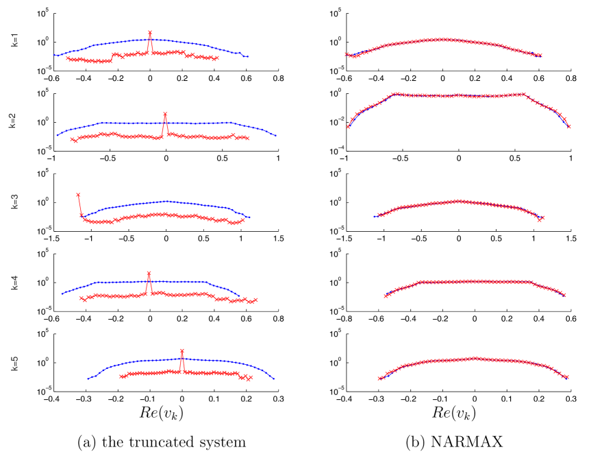
Figure 2: Semilog plot of the probability density functions reproduced by the truncated system and by the NARMAX system (red $\times$’s), compared to the full system (blue dots). Here we only plot the real parts of the paths of the Fourier modes (from top to bottom, the wave numbers are $k=1,2,\dots,5$). Note the distributions of the truncated system are not symmetric because solutions appear to converge to a fixed point, so that our ergodicity assumption is invalid.

The pdfs and autocorrelation functions of data are reproduced well by the NARMAX reduced system, as shown in Figure 2 and Figure 3. The NARMAX system reproduces almost exactly the pdfs and the autocorrelation functions of the data, a significant improvement over the truncated system.

We also computed energy covariances ${\rm cov}(|v_{k}|^{2},|v_{\ell}^{2}|)$ for some pairs $(k,\ell)$ with $k\neq\ell$. (Recall from section 2 that this is expected to be nonzero.) In particular, tests with $k=2$ and $\ell\in\{1,2,3,4,5\}$ show that the NARMAX reduced system can correctly capture these energy-energy covariances, whereas the truncated system does not (data not shown).

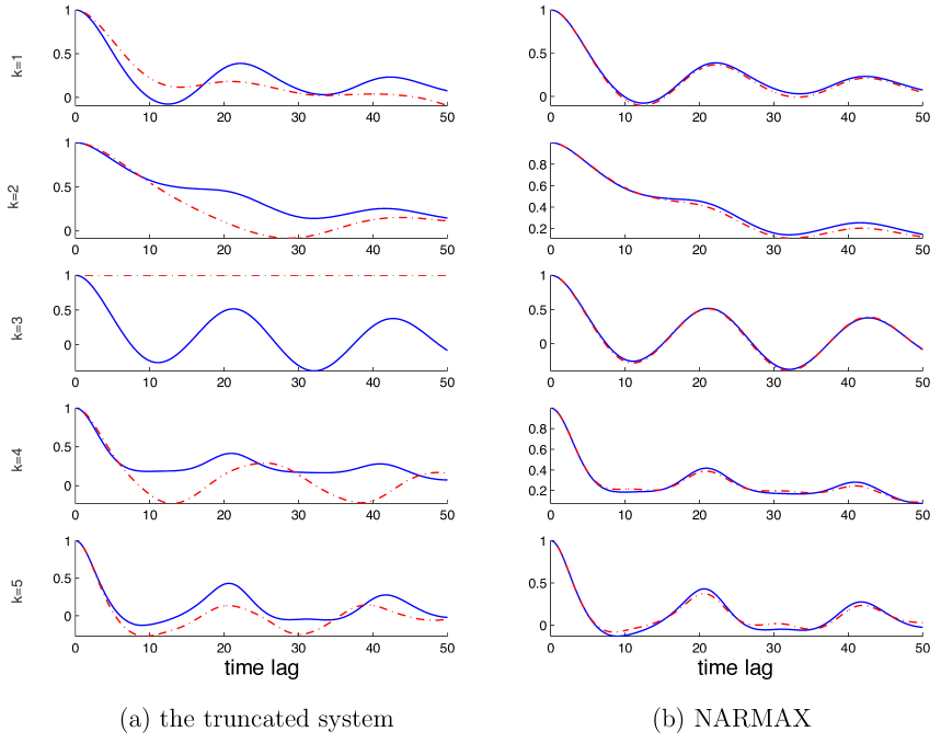
Figure 3: The autocorrelation functions reproduced by the truncated system and and the NARMAX system (dot dash line), compared to the full system (solid line). Here we only plot the real parts of the paths of the Fourier modes (from top to bottom, the wave numbers are $k=1,2,\dots,5$).

5.3 Short-term forecasting

We now investigate how well the NARMAX reduced system predicts the behavior of the full system.

We start from single path forecasts. For the NARMAX with orders $(p,r,q)$, we start the multistep recursion by using an initial segment with $m=2\max\{p,r,q\}+1$ steps as follows. We set $\xi^{1}=\cdots=\xi^{q}=0$, and estimate $\xi^{q+1},\dots,\xi^{m}$ using equation (11). Then we follow the discrete system to generate an ensemble of trajectories from different realizations, with all realizations using the same initial condition. We do not introduce artificial perturbations into the initial conditions, because the exact initial conditions are known. A typical ensemble of $20$ trajectories, as well as its mean trajectory and the corresponding data trajectory, is shown in Figure 4(b). As a comparison, we also plot a forecast using the truncated system. Since the observations provide the exact initial condition, the truncated system produces a single forecast path, see Figure 4(a). We observe that the ensemble of NARMAX follows the true trajectory well for about 50 time units, and the spread becomes wide quickly afterwards, while the ensemble mean can follow the true trajectory to 55 time units. Compared to the truncated system which can make forecast for about 20 time units, NARMAX can make forecast for about 55 time units, which is a significant improvement. We comment that in the prediction time is about 35 time units in [43], where the Mori-Zwanzig formalism is used.

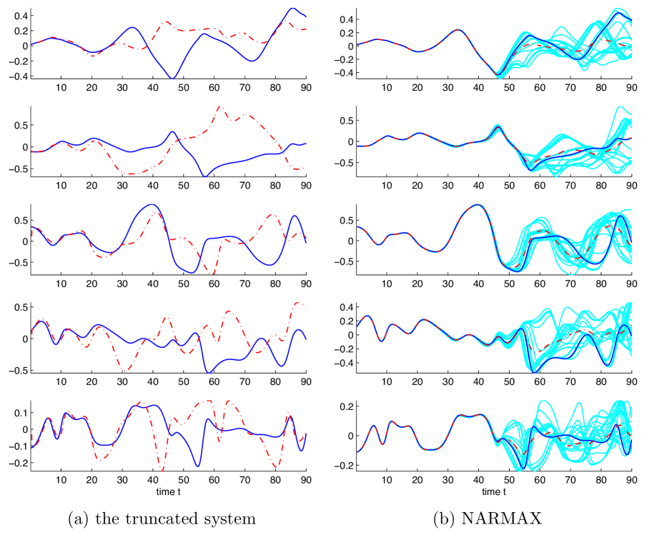
Figure 4: A typical path forecast made by the reduced systems compared to the data (solid line). (a) the truncated system (dot-dashed line); (b) ensemble trajectories (cyan line) and the mean trajectory of the ensemble (dot-dashed line) of the NARMAX system. Here we only plot the real parts of the paths of the Fourier modes (from top to bottom, the wave numbers are $k=1,\cdots,5$).

To measure the reliability of the forecast as a function of lead time, we compute two commonly-used statistics, the root-mean-square-error (RMSE) and the anomaly correlation (ANCR). Both statistics are based on generating a large number of ensembles of trajectories of the reduced system starting from different initial conditions, and comparing the mean ensemble predictions with the true trajectories, as follows.

First we take $N_{0}$ short pieces of the data, $\left\{\left(v(t_{n}),n=n_{i},n_{i}+1,\dots,n_{i}+T\right)\right\}_{i=1}^{N_{0}}$ with $n_{i+1}=n_{i}+T_{lag}/\delta$, where $T=$ $T_{lag}/\delta$ is the length of each piece and $T_{lag}$ is the time gap between two adjacent pieces. For each short piece of data $\left(v(t_{n}),n=n_{i},\dots,n_{i}+T\right)$, we generate $N_{ens}$ trajectories of length $T$ from the NARMAX reduced system, starting all ensemble members from the same several-step initial condition $\left(v(t_{n_{i}}),v(t_{n_{i}+1}),\dots,v(t_{n_{i}+m})\right)$, where $m=2\max\left\{p,r,q\right\}+1$, and denote the sample trajectories by $\left(u^{n}(i,j),n=1,\dots,T\right)$ for $i=1,\dots,N_{0}$ and $j=1,\dots,N_{ens}$. Again, we do not introduce artificial perturbations into the initial conditions, because the exact initial conditions are known, and by initializing from data, we preserve the memory of the system so as to generate better ensemble trajectories.

We then calculate the mean trajectory for each ensemble, $\bar{u}^{n}(i)=\frac{1}{N_{ens}}\sum_{j=1}^{N_{ens}}u^{n}(i,j)$. The RMSE measures, in an average sense, the difference between the mean ensemble trajectory, i.e., the expected path predicted by the reduced model, and the true data trajectory:

$$\mathrm{RMSE}(\tau_{n}):=\left(\frac{1}{N_{0}}\sum_{i=1}^{N_{0}}\left|\operatorname{Re}v(t_{n_{i}+n})-\operatorname{Re}\bar{u}^{n}(i)\right|^{2}\right)^{1/2},$$

where $\tau_{n}=n\delta$. The anomaly correlation (ANCR) shows the average correlation between the mean ensemble trajectory and the true data trajectory (see e.g [12]):

$$\mathrm{ANCR}(\tau_{n}):=\frac{1}{N_{0}}\sum_{i=1}^{N_{0}}\frac{\mathbf{a}^{v,i}(n)\cdot\mathbf{a}^{u,i}(n)}{\sqrt{|\mathbf{a}^{v,i}(n)|^{2}\left|\mathbf{a}^{u,i}(n)\right|^{2}}},$$

where $\mathbf{a}^{v,i}(n)=\operatorname{Re}v(t_{n_{i}+n})-\operatorname{Re}\left\langle v\right\rangle$ and $\mathbf{a}^{u,i}(n)=\operatorname{Re}\bar{u}^{n}(i)-\operatorname{Re}\left\langle v\right\rangle$ are the anomalies in data and the ensemble mean. Here $\mathbf{a\cdot b=}\sum_{k=1}^{K}a_{k}b_{k}$, $\left|\mathbf{a}\right|^{2}=\mathbf{a\cdot a}$, and $\left\langle v\right\rangle$ is the time average of the long trajectory of $v$. Both statistics measure the accuracy of the mean ensemble prediction; $\rm{RMSE}=0$ and $\rm{ANCR}=1$ would correspond to a perfect prediction, and small RMSEs and large (close to 1) ANCRs are desired.

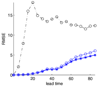
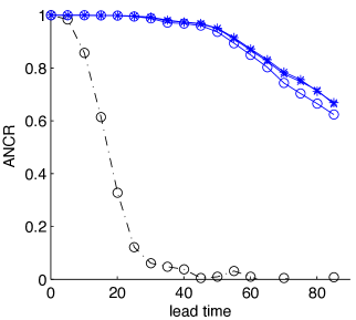
(a) RMSE	(b) ANCR

Figure 5: Root-mean-square-error (RMSE) and Anomaly correlations (ANCR) of ensemble forecasting, produced by the NARMAX system (solid lines) and the truncated system (dot dashed line), for different ensemble sizes: $N_{ens}=1$ (circle marker), $N_{ens}=5$ (cross marker), and $N_{ens}=20$ (asterisk marker).

Results for RMSE and ANCR for $N_{0}=1000$ ensembles are shown in Figure 5, where we tested three ensemble sizes: $N_{ens}=1,5,20$. The forecast lead time at which the RMSE keeps below 2 is about 50 time units, which is about 10 times of the forecast lead time of the truncated system. The forecast lead time at which the ANCR drops below 0.9 is about 55 time units, which is about five times of number of the truncated system. We also observe that a larger ensemble size leads to smaller RMSEs and larger ANCRs.

5.4 Importance of the nonlinear terms in NARMAX

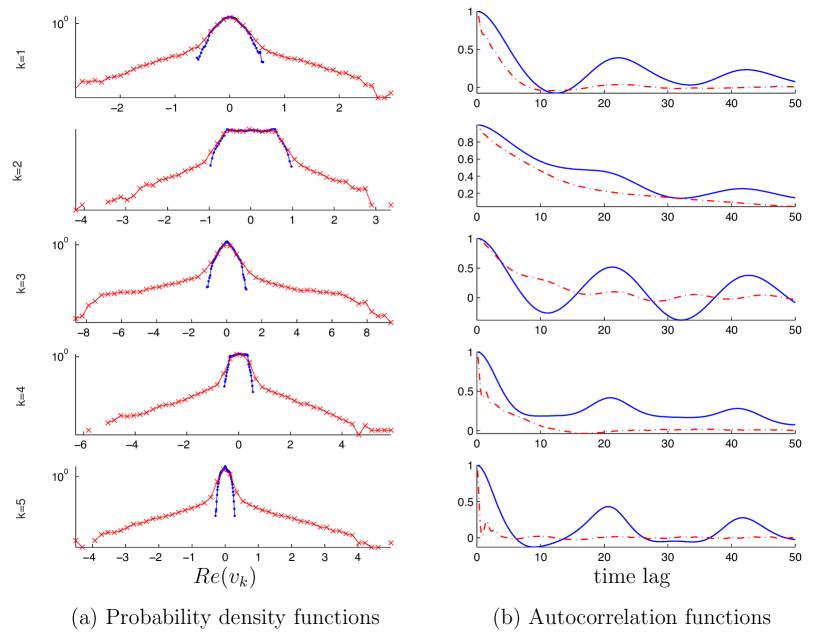
Figure 6: Results produced by ARMAX, i.e., using only linear terms in the ansatz for $z^{n}$. In (a), we compare the probability density functions of different modes produced by ARMAX (red $\times$’s) to that of the full model (blue dots). In (b), we compare the autocorrelation functions (solid line for full model, dashed line for ARMAX). Compare to Figures 2(b) and 3(b).

Finally, we examine the necessity of including nonlinear terms in the ansatz, by comparing NARMAX to ARMAX, i.e., stochastic parametrization keeping only the linear terms in the ansatz. We performed a number of numerical experiments in which we fitted an ARMAX ansatz to data. We found that for $(p,r,q)=(0,2,1)$, which was the best order we found for NARMAX, the corresponding ARMAX approximation was unstable.

We also found the best orders for ARMAX to be stable, which were $(p,r,q)=(2,1,0)$, and compared the results to those produced by NARMAX. The results are shown in Figure 6. In (a), the pdfs are shown for each resolved Fourier mode, and compared to those of the full model. Clearly, the Fourier modes for ARMAX experience much larger fluctuations, presumably because of the build-up of energy in the resolved modes. In contrast, the results produced by NARMAX match reality much better (see Figures 2(b)), as it more correctly models the nonlinear interactions between different modes. A consequence of these larger fluctuations is that ARMAX cannot even capture the mean energy spectrum: the ARMAX model leads to mean energies that are about 5 times larger than the true energy spectrum, which NARMAX is able to reproduce (data not shown).

Figure 6(b) shows the corresponding autocorrelations. We see that ARMAX does not correctly capture the temporal structure of the dynamics. Again, this is consistent with the fact that in ARMAX the components of $z^{n}$ are independent, which do not correctly capture the energetics the KSE. In contrast, the NARMAX results in Figure 3(b) show a much better match.

6 Conclusions and discussion

We performed a stochastic parametrization for the KSE equation in order to use it as a test bed for developing such parametrization for more complicated systems. We estimated and identified the model error in a discrete-time setting, which made the inference from data easier, and avoided the need to solve nonlinear stochastic differential systems; we then represented the model error as a NARMAX time series. We found an efficient form for the NARMAX series with the help of an approximate inertial manifold, which we determined by a construction developed in a continuum setting, and which we improved by parametrizing its coefficients.

A number of dimensional reduction techniques have been developed over the years in the continuum setting, e.g., inertial manifolds, renormalization groups, the Mori-Zwanzig formalism, and a variety of perturbation-based methods. In the present paper we showed, in the Kuramoto-Sivashinsky case, that continuum methods could be adapted for use in the more practical discrete-time setting, where they could help to find an effective structure for the NARMAX series, and could in turn be enhanced by estimating the coefficients that appear, producing an effective and relatively simple parametrization. Another example in a similar spirit was provided by Stinis [44], who renormalized coefficients in a series implementation of the Mori-Zwanzig formalism.

Such continuous/discrete, analytical/numerical hybrids raise interesting questions. Do there exist general, systematic ways to use continuum models to identify terms in NARMAX series? Does the discrete setting require in general that the continuum methods be modified or discretized? What are the limitations of this approach? The answers await further work.

7 Acknowledgements

The authors thank the anonymous referee, Prof. Panos Stinis, and Prof. Robert Miller for their helpful suggestions. KL is supported in part by the National Science Foundation under grants DMS-1217065 and DMS-1418775, and thanks the Mathematics Group at Lawrence Berkeley National Laboratory for facilitating this collaboration. AJC and FL are supported in part by the Director, Office of Science, Computational and Technology Research, U.S. Department of Energy, under Contract No. DE-AC02-05CH11231, and by the National Science Foundation under grants DMS-1217065 and DMS-1419044.

References

- [1] H.M. Arnold, I.M. Moroz, and T.N. Palmer. Stochastic parametrization and model uncertainty in the Lorenz’96 system. Phil. Trans. R. Soc. A, 371:20110479, 2013.
- [2] S.A. Billings. Nonlinear System Identification: NARMAX Methods in the Time, Frequency, and Spatiotemporal Domains. John Wiley and Sons, 2013.
- [3] P. Brockwell and R. Davis. Introduction to Time Series and Forecasting. Springer, New York, NY, 2002.
- [4] J.C. Bronski and T.N. Gambill. Uncertainty estimates and L2 bounds for the Kuramoto-Sivashinsky equation. Nonlinearity, 19(9):2023, 2006.
- [5] M.D. Chekroun, D. Kondrashov, and M. Ghil. Predicting stochastic systems by noise sampling, and application to the El Niño-Southern Oscillation. Proc. Natl. Acad. Sci. USA, 108:11766–11771, 2011.
- [6] A.J. Chorin and O.H. Hald. Stochastic Tools in Mathematics and Science. Springer, New York, NY, 3rd edition, 2013.
- [7] A.J. Chorin and O.H. Hald. Estimating the uncertainty in underresolved nonlinear dynamics. Math. Mech. Solids, 19(1):28–38, 2014.
- [8] A.J. Chorin, O.H. Hald, and R. Kupferman. Optimal prediction with memory. Physica D, 166(3):239–257, 2002.
- [9] A.J. Chorin and F. Lu. Discrete approach to stochastic parametrization and dimension reduction in nonlinear dynamics. Proc. Natl. Acad. Sci. USA, 112(32):9804–9809, 2015.
- [10] P. Constantin, C. Foias, B. Nicolaenko, and R. Temam. Integral Manifolds and Inertial Manifolds for Dissipative Partial Differential Equations. Applied Mathematics Sciences, No. 70. Springer, Berlin, 1988.
- [11] S.M. Cox and P.C. Matthews. Exponential time differencing for stiff systems. J. Comput. Phys., 176(2):430–455, 2002.
- [12] D. Crommelin and E. Vanden-Eijnden. Subgrid-scale parameterization with conditional Markov chains. J. Atmos. Sci, 65(8):2661–2675, 2008.
- [13] F. Ding and T. Chen. Identification of Hammerstein nonlinear ARMAX systems. Automatica, 41(9):1479–1489, 2005.
- [14] A. Du and J. Duan. A stochastic approach for parameterizing unresolved scales in a system with memory. J Algorithm Comput Technol., 3(3):393–405, 2009.
- [15] J. Duan and B. Nadiga. Stochastic parameterization for large eddy simulation of geophysical flows. Proc. Amer. Math. Soc., 135(4):1187–1196, 2007.
- [16] J.-P. Eckmann and D. Ruelle. Ergodic theory of chaos and strange attractors. Rev. Mod. Phys., 57(3):617, 1985.
- [17] J. Fan and Q. Yao. Nonlinear Time Series: Nonparametric and Parametric Methods. Springer, New York, NY, 2003.
- [18] C. Foias, O. Manley, and R. Temam. Modelling of the interaction of small and large eddies in two dimensional turbulent flows. RAIRO-Modélisation mathématique et analyse numérique, 22(1):93–118, 1988.
- [19] J. Goodman. Stability of the Kuramoto-Sivashinsky and related systems. Comm. Pure Appl. Math., 47(3):293–306, 1994.
- [20] D. Gottlieb and S. Orszag. Numerical Analysis of Spectral Methods: Theory and Applications. SIAM, Philadelphia, 1977.
- [21] J.D. Hamilton. Time Series Analysis. Princeton University Press, Princeton, NJ, 1994.
- [22] E.J. Hannan. The identification and parameterization of ARMAX and state space forms. Econometrica, 44:713–723, 1976.
- [23] J. Harlim. Model error in data assimilation. In C.L.E. Franzke and T.J. O’Kane, editors, Nonlinear and Stochastic Climate Dynamics, page in press. Cambridge University Press, Oxford, 2016.
- [24] J.M. Hyman and B. Nicolaenko. The Kuramoto-Sivashinsky equation: a bridge between PDE’s and dynamical systems. Physica D, 18(1):113–126, 1986.
- [25] M.S. Jolly, I. G. Kevrekidis, and E. S. Titi. Approximate inertial manifolds for the Kuramoto-Sivashinsky equation: analysis and computations. Physica D, 44(1):38–60, 1990.
- [26] M.S. Jolly, I.G. Kevrekidis, and E.S. Titi. Preserving dissipation in approximate inertial forms for the Kuramoto-Sivashinsky equation. J. Dynam. Differential Equations, 3(2):179–197, 1991.
- [27] M.S. Jolly, R. Rosa, and R. Temam. Evaluating the dimension of an inertial manifold for the Kuramoto-Sivashinsky equation. Adv. Differential Equ., 5(1-3):31–66, 2000.
- [28] A.K. Kassam and L.N. Trefethen. Fourth-order time stepping for stiff PDEs. SIAM J. Sci. Comput., 26(4):1214–1233, 2005.
- [29] P.E. Kloeden and E. Platen. Numerical Solution of Stochastic Differential Equations. Springer, Berlin, 3rd edition, 1999.
- [30] D. Kondrashov, M.D. Chekroun, and M. Ghil. Data-driven non-Markovian closure models. Physica D, 297:33–55, 2015.
- [31] F. Kwasniok. Data-based stochastic subgrid-scale parametrization: an approach using cluster-weighted modeling. Phil. Trans. R. Soc. A, 370:1061–1086, 2012.
- [32] A.J. Majda and J. Harlim. Physics constrained nonlinear regression models for time series. Nonlinearity, 26(1):201–217, 2013.
- [33] G.N. Milstein and M.V. Tretyakov. Stochastic Numerics for Mathematical Physics. Springer-Verlag, 2004.
- [34] S.A. Orszag. On the elimination of aliasing in finite-difference schemes by filtering high-wavenumber components. J. Atmos. Sci., 28(6):1074–1074, 1971.
- [35] T. N. Palmer. A nonlinear dynamical perspective on model error: A proposal for non-local stochastic-dynamic parametrization in weather and climate prediction models. Q. J. Roy. Meteror. Soc., 127(572):279–304, 2001.
- [36] Y. Pokern, A.M. Stuart, and P. Wiberg. Parameter estimation for partially observed hypoelliptic diffusions. J. Roy. Statis. Soc. B, 71(1):49–73, 2009.
- [37] J.C. Robinson. Inertial manifolds for the Kuramoto-Sivashinsky equation. Phys. Lett. A,, 184(2):190–193, 1994.
- [38] R. Rosa. Approximate inertial manifolds of exponential order. Discrete Contin. Dynam. Systems, 3(1):421–448, 1995.
- [39] M. Rost and J. Krug. A particle model for the kuramoto-sivashinsky equation. Physica D, 88(1):1–13, 1995.
- [40] A. Samson and M. Thieullen. A contrast estimator for completely or partially observed hypoelliptic diffusion. Stochastic Process. Appl., 122(7):2521–2552, 2012.
- [41] M. Schmuck, M. Pradas, S. Kalliadasis, and G.A. Pavliotis. New stochastic mode reduction strategy for dissipative systems. Phys. Rev. Lett., 110(24):244101, 2013.
- [42] M. Schmuck, M. Pradas, G.A. Pavliotis, and S. Kalliadasis. A new mode reduction strategy for the generalized Kuramoto–Sivashinsky equation. IMA J. Appl. Math., 80(2):273–301, 2015.
- [43] P. Stinis. Stochastic optimal prediction for the Kuramoto–Sivashinsky equation. Multiscale Modeling Simul., 2(4):580–612, 2004.
- [44] P. Stinis. Renormalized Mori–Zwanzig reduced models for systems without scale separation. Proc. R. Soc. A, 471:20140446, 2015.
- [45] R. Temam and X. Wang. Estimates on the lowest dimension of inertial manifolds for the Kuramoto-Sivashinsky equation in the general case. Differ. Integral Equ., 7(3-4):1095–1108, 1994.
- [46] S. Toh. Statistical model with localized structures describing the spatio-temporal chaos of Kuramoto-Sivashinsky equation. J. Phys. Soc. Jpn., 56(3):949–962, 1987.
- [47] D.S. Wilks. Effects of stochastic parameterizations in the Lorenz’96 system. Q. J. R. Meteorol. Soc., 131(606):389–407, 2005.
- [48] V. Yakhot. Large-scale properties of unstable systems governed by the Kuramoto-Sivashinksi equation. Phys. Rev. A, 24(1):642, 1981.
- [49] L.-S. Young. Mathematical theory of Lyapunov exponents. J. Phys. A Math. Theor., 46(25):254001, 2013.
- [50] R. Zwanzig. Nonequilibrium Statistical Mechanics. Oxford University Press, USA, 2001.