Detecting the Supernova Breakout Burst in Terrestrial Neutrino Detectors

Abstract

We calculate the distance-dependent performance of a few representative terrestrial neutrino detectors in detecting and measuring the properties of the $\nu_{e}$ breakout burst light curve in a Galactic core-collapse supernova. The breakout burst is a signature phenomenon of core collapse and offers a probe into the stellar core through collapse and bounce. We examine cases of no neutrino oscillations and oscillations due to normal and inverted neutrino-mass hierarchies. For the normal hierarchy, other neutrino flavors emitted by the supernova overwhelm the $\nu_{e}$ signal, making a detection of the breakout burst difficult. For the inverted hierarchy (IH), some detectors at some distances should be able to see the $\nu_{e}$ breakout burst peak and measure its properties. For the IH, the maximum luminosity of the breakout burst can be measured at 10 kpc to accuracies of $\sim$30% for Hyper-Kamiokande (Hyper-K) and $\sim$60% for the Deep Underground Neutrino Experiment (DUNE). Super-Kamiokande (Super-K) and Jiangmen Underground Neutrino Observatory (JUNO) lack the mass needed to make an accurate measurement. For the IH, the time of the maximum luminosity of the breakout burst can be measured in Hyper-K to an accuracy of $\sim$3 ms at 7 kpc, in DUNE $\sim$2 ms at 4 kpc, and JUNO and Super-K can measure the time of maximum luminosity to an accuracy of $\sim$2 ms at 1 kpc. Detector backgrounds in IceCube render a measurement of the $\nu_{e}$ breakout burst unlikely. For the inverted hierarchy, a measurement of the maximum luminosity of the breakout burst could be used to differentiate between nuclear equations of state.

1. Introduction

The core-collapse supernova (CCSN) explosion mechanism is a long-standing unsolved problem in astrophysics. Extant CCSN models universally indicate that neutrino emission is a key aspect of a CCSN, with $\sim$99% of a CCSN’s energy carried away by neutrinos. Such a neutrino signature was confirmed in broad outline by the detection of neutrinos from SN 1987A (Bionta et al., 1987; Hirata et al., 1987). Since the events that lead to a CCSN are entirely contained in the obscured core of the exploding star, the measurement of neutrinos (which are able to stream from the core of a star) is vital for testing CCSN theory.

CCSNe occur as successive stages of nuclear burning build a degenerate core to the Chandrasekhar limit. At this point, the core collapses in on itself. During collapse, electron capture causes the core to become neutron-rich. The implosion of the core proceeds until the material reaches densities near nuclear, at which point the implosion rebounds and produces an outward-propagating shock wave. As the shock propagates, it causes nuclei to dissociate. Electron capture on the now-free protons produces a large number of $\nu_{e}$’s in the region behind the shock. Initially, the optical depth seen by these neutrinos prevents their escape from the star, but as the shock crosses the $\nu_{e}$-neutrinospheres, the $\nu_{e}$’s produced by the shock (as well as $\nu_{e}$’s produced previously that have diffused to the neutrinosphere) create a very luminous (${\sim}3.5\times 10^{53}$ erg s^-1) spike (“breakout burst”) in the $\nu_{e}$ emission, which lasts for ${\sim}10$ ms. After this breakout spike, neutrinos of all types radiate from the proto-neutron star for ${\sim}10$ s or more (Burrows & Lattimer 1986). Neutrino oscillations are likely to convert the $\nu_{e}$’s of the breakout burst partially or entirely to other neutrino flavors (Mirizzi et al. 2015).

Prior to the $\nu_{e}$ breakout burst, there is a smaller $\nu_{e}$ luminosity peak due to $\nu_{e}$’s produced by the neutronization of the core during collapse. As the density and temperature of the core increase, the opacity increases and eventually these neutrinos are trapped, producing a peak and subsequent decrease in luminosity (“pre-breakout neutronization peak”). The peak luminosity reached is $\sim$5$\times 10^{52}$ erg s^-1.

The breakout burst of a CCSN is a signature phenomenon that must exist for current CCSN theories to be valid. Hence, unambiguous detection of the breakout burst in the next Galactic CCSN is vital to validating theory, and a measurement of the properties of the breakout burst would be important for testing and discriminating between CCSN models. Since Galactic CCSNe occur at a rate of $\sim$3 per century (Adams et al. 2013), to take advantage of the next Galactic CCSN, we must constantly be ready to take data. The Supernova Early Warning System (SNEWS) provides such constant vigilance (Antonioli et al., 2004; Scholberg, 2008).

The very property of neutrinos that allows them to stream through the stellar mantle also makes them very difficult to detect. Only 19 neutrinos were detected in the Kamiokande II and IMB detectors from SN 1987A (Bionta et al., 1987; Hirata et al., 1987). This was sufficient to confirm general details of CCSN theory but lacked sufficient discriminating power to truly differentiate between models, as well as lacked detail to see the $\nu_{e}$ breakout burst. The current generation of neutrino detectors promises much larger integral signals for a Galactic CCSN, but will they be adequately sensitive to detect and characterize the inaugural breakout burst? This work seeks to answer this question in the context of current and likely future neutrino detectors.

The CCSN models used for our analysis are introduced in Section 2, and the expected evolution of the detected breakout burst signal is discussed in Section 3. The various classes of neutrino detectors are discussed in Section 4. The method of our analysis is outlined in Section 5 and the results of our analysis are explored in Section 6 (which includes results from the no-oscillation case, as well as those due to the normal and inverse neutrino-mass hierarchies). We then conclude in Section 7.

2. The Supernova Models

The models used in this study were produced using Fornax (J. Dolence & A. Burrows 2015, in preparation). Fornax is a code written in generally covariant form for multidimensional, self-gravitating, radiation hydrodynamics that is second-order accurate in space and time and was designed from scratch with the CCSN problem in mind. The code solves the equations of compressible hydrodynamics with an arbitrary equation of state (EOS), coupled to the multigroup two-moment equations for neutrino transport. The hydrodynamics in Fornax is based on a directionally unsplit Godunov-type finite-volume method. Fluxes at cell faces are computed with the fast and accurate HLLC approximate Riemann solver, with left and right states given by limited parabolic reconstructions of the underlying volume-averaged states. The multigroup two-moment equations for neutrino transport are formulated in the comoving frame and include all terms to $\mathcal{O}$($v/c$). The moment hierarchy is closed with the “M1” model. Fornax adopts a Godunov-type approach for treating the transport-related divergence terms that requires that we solve a generalized Riemann problem at each face. All of the these transport-related terms are treated explicitly in time. After core bounce, the fastest hydrodynamic signal speeds in the CCSN problem are within a factor of a few of the speed of light, so explicit time integration is not only simpler and generally more accurate but it is also faster than globally coupled time implicit transport solves that are typically employed in radiation hydrodynamics. The source and sink terms that transfer energy between the radiation and the gas are operator-split and treated implicitly. These terms are purely local to each cell and do not introduce any global coupling.

Progenitors with mass of 12, 15, 20, and 25 $M_{\odot}$ from Woosley & Heger (2007) were simulated in 1D with the Lattimer–Swesty high-density nuclear EOS with $K=220$ MeV (LSEOS; Lattimer & Swesty 1991), while a progenitor with mass 15 $M_{\odot}$ was simulated using the Shen nuclear EOS (Shen EOS; Shen et al., 1998a, b). This set of models is chosen to give a good span of potential progenitors for an actual CCSN. Since in this study we focus on the breakout burst, the full ${\sim}10$ s of core neutrino cooling is not important for our study and is, thus, not discussed further.

Figure 1 shows the early (unoscillated) neutrino light curve for the neutrino species in the models: $\nu_{e}$, $\bar{\nu}_{e}$, and $\nu_{x}$ (which represents $\nu_{\mu}$, $\nu_{\tau}$, and their antiparticles collectively), with $L_{\nu_{i}}$ representing the $\nu_{i}$ energy luminosity. In this work, we use $\nu_{\mu,\nobreak\tau}$ to refer to $\nu_{\mu}$ and $\nu_{\tau}$ and use $\bar{\nu}_{\mu,\nobreak\tau}$ to refer to $\bar{\nu}_{\mu}$ and $\bar{\nu}_{\tau}$. Additionally, $L_{\nu_{x}}$ refers to the luminosity due to all of the $\nu_{x}$’s together, while $L_{\nu_{\mu,\nobreak\tau}}$ and $L_{\bar{\nu}_{\mu,\nobreak\tau}}$ refer to the luminosity due to just one of their constituent species. The initial peak in $\nu_{e}$ luminosity from the preshock neutronization of the core is evident, followed by the much steeper rise and larger peak in $\nu_{e}$ luminosity due to the breakout burst. After the breakout burst, the $\bar{\nu}_{e}$ and $\nu_{x}$ luminosities rise to nearly constant values. The $\nu_{e}$ luminosity then falls to a comparably constant value. In studying the breakout burst, $\bar{\nu}_{e}$ and $\nu_{x}$ serve as a background to the $\nu_{e}$ signal we want to detect.

Figure 2 shows the unoscillated-$\nu_{e}$ number luminosity as a function of time during breakout for the various models. The light curves are centered around their maximum values. The Shen EOS model has the largest peak luminosity, while the LSEOS models are grouped together at a slightly lower peak luminosity. Results from Sullivan et al. (2015) suggest that the higher peak $\nu_{e}$ luminosity and smaller light curve width associated with the Shen EOS are due to its smaller electron-capture rate (relative to that using the LSEOS), particularly on infall. The different electron-capture rates are due to different free proton abundances and nucleon chemical potentials, the latter of which also affect the stimulated absorption correction of electron capture. This tight grouping of peak luminosities for all progenitors, if in fact real, can be used as a standard candle to determine the distance to a supernova (SN). Kachelrieß et al. (2005) suggest that an SN at 10 kpc could have its distance determined to a precision of $\sim$5%, if these theoretical predictions play out.

The goal of our analysis here is to examine, for a given detector, for a given SN distance, how well the various properties of this breakout burst can be constrained based on expected neutrino signals, as well as determine whether our different CCSN models can be differentiated based on a measurement of the breakout burst. To quantify various properties of the breakout burst, we define the following physical parameters: the maximum number luminosity of breakout burst ($L^{n}_{\nu_{e},\mathrm{max}}$), the time of maximum luminosity ($t_{\mathrm{max}}$), the width of the breakout burst peak ($w$, calculated using the FWHM), the rise time ($t_{\mathrm{rise},1/2}$, calculated using the width left of peak at half-maximum), and the fall time ($t_{\mathrm{fall},1/2}$, calculated using the width right of peak at half-maximum). For the preshock neutronization peak we define the following physical parameters: the maximum number luminosity of the preshock peak ($L^{n}_{\nu_{e},\mathrm{max,pre}}$) and the time of this maximum luminosity ($t_{\mathrm{max,pre}}$). Table 1 shows the values the physical parameters of the breakout burst take in our number luminosity light curves, and Table 2 shows the values the physical parameters of the preshock neutronization peak take in the same curves. The fact that $t_{\mathrm{max}}=0$ for all models is to be expected, since the zero point in time for all the models is defined to be the time of maximum luminosity.

Table 1Physical Parameters of the Breakout Peak Fit to the Number Luminosity, L${}^{n}_{\nu_{e}}$

Model	$L^{n}_{\nu_{e},\mathrm{max}}$	$t_{\mathrm{max}}$	$w$	$t_{\mathrm{rise},1/2}$	$t_{\mathrm{fall},1/2}$
($M_{\odot}$)	$(10^{58}$ s${}^{-1})$	(ms)	(ms)	(ms)	(ms)
12	1.97	0.00	8.85	2.23	6.62
15	2.01	0.00	9.29	2.24	7.06
15 S	2.23	0.00	8.71	1.70	7.01
20	2.03	0.00	10.2	2.22	7.96
25	2.02	0.00	10.4	2.28	8.10

Table 2Physical Parameters of the Preshock Neutronization Peak Fit to the Number Luminosity, L${}^{n}_{\nu_{e}}$

Model	$L^{n}_{\nu_{e},\mathrm{max,pre}}$	$t_{\mathrm{max,pre}}$
($M_{\odot}$)	(1058 s-1)	(ms)
12	0.552	-6.51
15	0.577	-6.48
15 S	0.629	-5.73
20	0.597	-6.43
25	0.604	-6.48

We construct an analytic model for the main breakout peak of our numerical light curves similar to equation (10) of Burrows & Mazurek (1983). This analytic model will later be used to fit simulated observations of the $\nu_{e}$ breakout burst light curve to measure various physical parameters of the breakout burst. The function we use to fit the main peak is

$$L(t)=\frac{A}{((t-t_{c})/[\textrm{ms}])^{\alpha}}\exp\left[-\left(\frac{b}{t-t_{c}}\right)^{\beta}\right]+L_{\textrm{base}},$$ (1)

where $A$ is a scaling parameter with units of (for energy luminosity) erg s^-1 or (for number luminosity) s^-1, $b$ is a width parameter, $t$ is the time since the maximum $\nu_{e}$ number luminosity, $t_{c}$ is a number used to center the fit appropriately, $\alpha$ and $\beta$ are exponents similar to those used in Burrows & Mazurek (1983), and $L_{\textrm{base}}$ (in units of erg s^-1 for energy luminosity or s^-1 for number luminosity) is used to set the floor of the fit. Since the intent of Equation (1) is to provide a fit to our models for subsequent analysis, we do not spend much time in this work examining its physical significance. We refer readers to Burrows & Mazurek (1983) for a motivation of its functional form. We do note that the floor set by $L_{\textrm{base}}$ can be thought of as the level to which the $\nu_{e}$ luminosity decays as the luminosity source transitions from the electron capture that dominates the breakout burst to the accretion, deleptonization, and cooling phases of the proto-neutron star.

Table 3Breakout Peak Fit to the Energy Luminosity, L${}_{\nu_{e}}$

Model	$A$	$b$	$t_{c}$	$\alpha$	$\beta$	$L_{\textrm{base}}$
($M_{\odot}$)	$(10^{57}$ erg s${}^{-1})$	(ms)	(ms)			$(10^{53}$ erg s${}^{-1})$
12	0.620	12.2	-4.69	3.06	1.09	0.360
15	1.52	20.6	-4.33	3.20	0.849	0.418
15 S	1.00e14	6.65e8	-2.49	6.26	0.182	0.345
20	1.00e14	2.33e7	-3.47	6.96	0.220	0.501
25	2.33e5	7090	-3.69	4.91	0.349	0.511

Figure 3 displays the fits of Equation (1) to our numerical models. The fits match the numerical models quite well. The analytic fitting parameters to the energy luminosity of all the numerical models are given in Table 3, and the fitting parameters to the number luminosity of all the numerical models are given in Table 4. The Shen EOS model is represented by “S” in the “Model” column; those models not marked with an “S” use the LSEOS. This is a convention we take throughout this work. Two of the parameters ($A$ and $b$) show variation over many orders of magnitude across the fits of the different models. Because of this, we set a maximum value for $A$, which equates to (for energy luminosity) $10^{71}$ erg s^-1 and (for number luminosity) $10^{71}$ s^-1. The choice of this particular maximum value is arbitrary. It is based on our experience with the behavior of the fits with unbounded parameters. Since the fits are so good, and since we care about the physical parameters that are derived from the fits rather than the fit parameters themselves, we see no harm in doing this. Additionally, we force $\alpha$, $\beta$, $L_{\textrm{base}}$, and $A$ to be positive. We wish to emphasize that although the parameters of Table 3 vary to a large degree between models, the important consideration in our analysis is not the parameters themselves, but the characteristics of the fit they provide (i.e. the physical parameters introduced previously and shown in Table 1), so the fidelity of the fits in representing the numerical models is far more important than the values the fit parameters take. A reason for the large variation in the best-fit values of $A$ and $b$ is the very large, positive covariance between these two parameters. Since the specific values of these parameters are not important, we do not focus on the covariance data in this work.

Table 4Breakout Peak Fit to the Number Luminosity, L${}^{n}_{\nu_{e}}$

Model	$A$	$b$	$t_{c}$	$\alpha$	$\beta$	$L^{n}_{base}$
($M_{\odot}$)	$(10^{61}$ s${}^{-1})$	(ms)	(ms)			$(10^{57}$ s${}^{-1})$
12	3.29	16.3	-4.30	2.94	0.892	2.88
15	39.7	60.1	-3.90	3.39	0.621	3.35
15 S	1.00e10	2.71e7	-2.38	4.95	0.198	2.76
20	1.00e10	8.44e5	-3.31	5.68	0.251	3.92
25	5.18e9	4.89e5	-3.41	5.67	0.260	4.06

Additionally, we fit the preshock neutronization peak with a modified lognormal curve,

$$L(t)=C\exp\left(\frac{-(\ln(t^{\prime}-\theta)-\mu)^{2}}{2\sigma^{2}}\right)(t^{\prime}-\theta)^{-1},$$ (2)

where $t^{\prime}=-t/$[ms], $C$ is a scaling factor, and all the other parameters have their usual meaning in relation to the lognormal distribution: $\sigma$ is the standard deviation, $\theta$ is the location parameter, and $\mu$ is the median of the distribution. The best-fit values to the preshock energy luminosity for the various models are shown in Table 5, and Table 6 shows the best-fit values for the preshock number luminosity. Figure 3 displays the fits of Equation (2) to our numerical models. The physical parameters we define for the preshock neutronization peak are (as introduced previously) the maximum number luminosity of the preshock peak ($L^{n}_{\nu_{e},\mathrm{max,pre}}$) and the time of this maximum luminosity ($t_{\mathrm{max,pre}}$). The model values of these parameters are shown in Table 2. It is the fits themselves (Equations 1 and 2), with the appropriate fitting parameters, that we use as our baseline models for our analysis over the time ranges fitted by them, not the numerical data from Fornax. The numerical data are used in the time ranges not fitted by Equations 1 and 2 (i.e., the time ranges before to the pre-breakout neutronization peak and after the breakout burst).

Table 5Preshock Neutronization Peak Fit to the Energy Luminosity, L${}_{\nu_{e}}$

Model	$C$	$\sigma$	$\theta$	$\mu$
($M_{\odot}$)	(1053 erg s-1)
12	3.93	0.822	1.96	2.08
15	4.28	0.809	1.79	2.12
15 S	4.78	0.790	0.925	2.08
20	5.17	0.708	0.653	2.20
25	5.41	0.682	0.404	2.22

Table 6Preshock Neutronization Peak Fit to the Number Luminosity, L${}^{n}_{\nu_{e}}$

Model	$C$	$\sigma$	$\theta$	$\mu$
($M_{\odot}$)	(1058 s-1)
12	3.74	0.834	1.72	2.26
15	3.91	0.857	1.79	2.28
15 S	4.32	0.817	0.809	2.26
20	4.63	0.754	0.596	2.33
25	4.40	0.807	1.22	2.31

The energy spectrum of all neutrino types varies during the shock breakout. Figure 4 shows the $\nu_{e}$ energy spectrum as a function of time through the breakout burst for a specific model, the 15 $M_{\odot}$ LSEOS model, derived using Fornax. We define the average neutrino energy $\overline{E}_{\nu_{i}}$ as

$$\overline{E}_{\nu_{i}}(t)\equiv\frac{\int L_{\nu_{i}}(E_{\nu_{i}},t)~{}dE_{\nu}}{\int L_{\nu_{i}}(E_{\nu_{i}},t)/E_{\nu_{i}}~{}dE_{\nu_{i}}}.$$ (3)

Figure 5 shows the average neutrino energy as a function of time for all the models (with the zero point in time set to be the time of maximum number luminosity). All the models show the same general behavior. $\overline{E}_{\nu_{e}}$ increases from the onset of the breakout burst, peaks near $t_{\mathrm{max}}$, and then decays slightly. However, during the breakout, $\overline{E}_{\nu_{e}}$ does not change radically and is similar from model to model. There is a slight trend for the average $\nu_{e}$ energy during breakout to be slightly higher for the lower-mass progenitors. In addition, the Shen EOS results in a slightly higher mean $\nu_{e}$ energy than the LSEOS. In all cases, the average energy peaks $\lesssim$1 ms later than the maximum number luminosity.

3. Signal Evolution

In a neutrino detector, for a given neutrino detection channel, the expected number of detected neutrinos $N_{\textrm{det}}$ as a function of time is given by

$$N_{\textrm{det}}(t)=\frac{N_{t}}{4\pi D^{2}}\int\frac{dL_{\nu}(E_{\nu},t)}{dE_{\nu}}\frac{1}{E_{\nu}}\sigma(E_{\nu})\epsilon(E_{e})dE_{\nu},$$ (4)

where $N_{t}$ is the number of target particles inside the detector, $dL_{\nu}/dE_{\nu}$ is the energy luminosity spectrum of neutrinos, $E_{\nu}$ is the neutrino energy, $E_{e}$ is the energy of the final-state electron, $D$ is the distance between the detector and the SN, $\sigma$ is the interaction cross section, and $\epsilon$ is the efficiency of detection.

In a detector, there is not a one-to-one mapping between the energy of an interacting neutrino and the detected energy of the products. To understand exactly what a signal will look like in a detector, we have to understand how the spectrum of the detectable products relates to the spectrum of the incident neutrinos. The number of events produced in a specific channel with product $x$ with observed kinetic energy $E_{x}$ is

$$\frac{dN_{x}}{dE_{x}dE_{\nu}dt}=\frac{N_{t}}{4\pi D^{2}}\frac{dL_{\nu}(t,E_{\nu})}{dE_{\nu}}\frac{1}{E_{\nu}}\frac{d\sigma(E_{x}^{\prime},E_{\nu})}{dE_{x}^{\prime}},$$ (5)

where $E_{\nu}$ is the energy of the interacting neutrino, $E_{x}^{\prime}$ is the energy of the product (usually an electron or positron), and $t$ is the detector time (with light-travel time $D/c$ subtracted).

Neutrino oscillations that occur as a result of the Mikheyev–Smirnov–Wolfenstein (MSW) effect in the envelope of a star will likely alter the measured $\nu_{e}$ signal from the breakout burst. There are two main realms of flavor conversions to be considered in the $\nu_{e}$ breakout burst, connected with the two potential neutrino-mass hierarchies: the normal hierarchy (NH), where the $\nu_{3}$ mass eigenstate is of larger mass than either of $\nu_{1}$ or $\nu_{2}$; and the inverted hierarchy (IH), where the $\nu_{3}$ mass eigenstate is of smaller mass than either of $\nu_{1}$ or $\nu_{2}$. In the case of the NH, the observed luminosity of a neutrino species $L^{obs}_{\nu_{i}}$ is (Mirizzi et al. 2015)

$$L^{\textrm{obs}}_{\nu_{e}} =L_{\nu_{\mu,\tau}},$$ (6)

$$L^{\textrm{obs}}_{\bar{\nu}_{e}} =\cos^{2}{\theta_{12}}L_{\bar{\nu}_{e}}+\sin^{2}{\theta_{12}}L_{\bar{\nu}_{\mu,\tau}},$$ (7)

where $\theta_{12}$ is the 1, 2 mixing angle. We use $\sin^{2}{\theta_{12}}=0.308$ in this work (Olive et al. 2014). In the case of the IH, the observed luminosity of a neutrino species is (Mirizzi et al. 2015)

$$L^{\textrm{obs}}_{\nu_{e}} =\sin^{2}{\theta_{12}}L_{\nu_{e}}+\cos^{2}{\theta_{12}}L_{\nu_{\mu,\tau}},$$ (8)

$$L^{\textrm{obs}}_{\bar{\nu}_{e}} =L_{\bar{\nu}_{\mu,\tau}}.$$ (9)

4. Terrestrial Neutrino Detectors

There are four main classes of detectors relevant for detecting the $\nu_{e}$ breakout burst: ⁴⁰Ar detectors, water-Cherenkov detectors, long-string detectors, and scintillation detectors. Each of these detector classes has its own strengths and weaknesses with regard to the detection of the breakout burst.

Table 7 lists the detectors we highlight in our study, as well as some other detectors of interest for detection of the breakout burst. It consists of both detectors currently running and detectors that are expected to come online in the coming years. The list is not exhaustive, but is rather a representative “short list” of detectors we think will provide the best opportunity to examine the breakout burst. We now discuss specifics of each class of detector.

Table 7Selected Neutrino Detectors

Detector	Detection Medium	Mass	Status
		(ktonne)
DUNE	40Ar	40	planning
Hyper-K	water	560 (fiducial)	proposed
Super-K	water	22.5 (fiducial)	running
IceCube	water ice	$\sim$900	running
JUNO	scintillator	20	construction
ICARUS	40Ar	.476 (active)	being refurbished
KamLAND	scintillator	1	running
LVD	scintillator	$\sim$1	running
NO$\nu$A	scintillator	14	running

4.1. ⁴⁰Ar Detectors

Of all the detector types we consider, ⁴⁰Ar detectors have the highest sensitivity to $\nu_{e}$’s (the primary neutrino emission of the breakout burst, ignoring oscillations). The $\nu_{e}$’s interact with ⁴⁰Ar nuclei via charged-current (CC) capture; it is the large cross section of this interaction that gives ⁴⁰Ar detectors such great $\nu_{e}$ sensitivity. The electron created in this process deposits its kinetic energy along an ionization trail through the detection medium. The ⁴⁰Ar detectors we mention in this paper are all time-projection chambers (TPCs). In a TPC, a voltage is applied across the detection medium, causing the particles ionized by the product electrons to drift toward a wire mesh that (when combined with the timing of the formation of the ionization trail) gives spatial information about the interaction inside the detector. The $\bar{\nu}_{e}$’s also undergo CC absorption with the ⁴⁰Ar nuclei. The cross section for this interaction, for the neutrino energies in an SN, is 2–3 orders of magnitude smaller than for $\nu_{e}$ CC absorption in the energy range relevant for this study, and so this interaction serves as a small background to the $\nu_{e}$ signal in the case of no oscillations. Neutrinos of all flavors can also be detected via elastic scattering off the electrons. Electrons produced from electron scattering are indistinguishable from the electrons produced by CC absorption of $\nu_{e}$’s on the ⁴⁰Ar nuclei, but electron scattering has a much smaller cross section (factor of ${\sim}100$ for 10 MeV neutrinos) than the CC interaction channel on ⁴⁰Ar. Because of the dominance of the cross sections through which $\nu_{e}$’s are detected and the dominance of the $\nu_{e}$ flux relative to the $\bar{\nu}_{e}$ and $\nu_{x}$ flux through the breakout burst, we assume the ability of these detectors to separate or ignore the background $\bar{\nu}_{e}$ and $\nu_{x}$ signals and consider only the $\nu_{e}$ luminosity in our analysis for the case of no neutrino oscillations. The mixing of the $\nu_{\mu,\nobreak\tau}$ and $\nu_{e}$ flux in the case of neutrino oscillations complicates this and we cannot assume, for either the NH or IH, that the $\nu_{\mu,\nobreak\tau}$ backgrounds are negligible. Also, ⁴⁰Ar detectors can measure the energies of the electrons produced in the neutrino interactions inside them. In principle, gamma rays from nuclear de-excitation could be detected, allowing the tagging of $\nu_{e}$ CC absorption events and their separation from electron-scattering events, as well as detection of neutral-current (NC) scatterings off of nuclei. The detectability of these gamma rays is still under study (A. Rubbia 2015, private communication), and we do not assume the ability to detect them.

The largest ⁴⁰Ar detector operated so far is ICARUS (Imaging Cosmic And Rare Underground Signals), formerly located in the Gran Sasso underground laboratory in Italy. The detector had an active mass of 476 tonnes (Rubbia et al. 2011). The detector is currently in the process of being refurbished for later installation in the USA at Fermilab. In our analysis, we assume a detection efficiency of 100% across all product energies for the ⁴⁰Ar detectors. We note that the interaction cross sections set their own threshold for neutrino detection, which is incorporated with our cross-section calculations. We refer interested readers to the Appendix for a further discussion of these cross sections. We calculate that a detector of ICARUS’s size will detect $\sim$1 $\nu_{e}$ in a 10 ms period over the breakout burst at a distance of 10 kpc in the case of no neutrino oscillations (even less in either NH- or IH-case oscillations). Because of the expected small signal from ICARUS, we do not use it in our analysis.

There are plans for a 40 ktonne (fiducial) ⁴⁰Ar detector to be constructed at the Sanford Lab in the Homestake Mine in South Dakota as a part of part of the Deep Underground Neutrino Experiment (DUNE; Goodman 2015). We calculate that an ⁴⁰Ar detector of this size will detect $\sim$120 $\nu_{e}$’s in a 10 ms period over the breakout burst at a distance of 10 kpc in the case of no neutrino oscillations. For the same situation as just outlined, the number of detected (original) $\nu_{e}$’s in the NH case will be $\sim$2 and in the IH case will be $\sim$40. The timing resolution of DUNE depends on its photon detection capabilities. We assume a DUNE that will have timing much better than the time bin width used in our analysis (1 ms).

4.2. Water-Cherenkov detectors

Water-Cherenkov detectors are large tanks of purified water primarily sensitive to $\bar{\nu}_{e}$’s through inverse $\beta$ decay (IBD) on protons (hydrogen nuclei): $\bar{\nu}_{e}+p\rightarrow e^{+}+n$. The positron produced by IBD emits Cherenkov light, which is detected by a photomultiplier tube (PMT) array placed around the detection volume. Neutrinos of all flavors can be detected through elastic scattering on electrons, $\nu_{i}+e^{-}\rightarrow\nu_{i}+e^{-}$. The final-state electrons are detected through their Cherenkov emission. $\nu_{e}$ and $\bar{\nu}_{e}$ can also undergo CC absorption on the oxygen nuclei and are detected through the electrons/positrons formed in these interactions, as well as through photons emitted via nuclear de-excitation. Additionally, neutrinos of all types may undergo NC interactions with the oxygen nuclei, which (if the interaction puts the nucleus in an excited state) can be detected by the photon emitted upon de-excitation of the nucleus.

In standard water-Cherenkov detectors, positrons from IBDs and electrons from electron scatterings can be statistically distinguished by the forward-peaked directionality of the electron-scattering products and the nearly isotropic products of IBD. The IBD detection channel has the largest cross section and so dominates when there is a $\bar{\nu}_{e}$ flux. Figure 1 shows that the $\bar{\nu}_{e}$ flux is not significant until after the $\nu_{e}$ peak of the breakout burst. Thus, previous to this, almost all detections can be attributed to $\nu_{e}$’s (in the no-oscillation case). After this the $\bar{\nu}_{e}$’s (and, less so, the $\nu_{x}$’s) must be accounted for. It is also possible to employ gadolinium (Gd) in water-Cherenkov detectors to tag the final-state neutrons and allow the IBD and electron elastic scattering signals to be separated (Vagins 2012; Laha & Beacom 2014). The large neutron capture cross section of Gd allows neutrons formed in IBD events to be quickly ($\sim$20 $\mu$s) captured, emitting three to four gamma rays with a total energy of 8 MeV (Beacom & Vagins 2004). The coincidence of a neutrino detection and a gamma ray from neutron capture on Gd allows the neutrino detection to be associated with an IBD. We assume the presence of Gd in our analysis. In practice, using Gd to tag IBD events will not be perfect, although the fraction of neutrons that are captured onto Gd is very high even for modest additions of Gd to water (Beacom & Vagins 2004). The signal remaining from untagged IBDs can be statistically subtracted from the remaining signal. Because of this, and because of the ability to statistically distinguish $\nu_{e}$’s and $\bar{\nu}_{e}$’s based on direction, in our analysis we assume that IBDs can be separated from the rest of the signal. In the case of no oscillations, this leaves the $\nu_{e}$ flux dominant. Laha & Beacom (2014) also state that $\nu_{x}$ information from scintillation detectors will allow those events to be statistically subtracted, leaving only the $\nu_{e}$ events. Based on this, we assume the ability to subtract or ignore all $\bar{\nu}_{e}+\nu_{x}$ backgrounds in the no-oscillation case. In the case of neutrino oscillations, the detectability of the background $\nu_{x}$ flux will increase and cannot be so easily ignored.

Super-Kamiokande (Super-K) is a 22.5 ktonne (fiducial) water-Cherenkov detector located in the Kamioka Mine in Japan (Fukuda et al., 2003; Ikeda et al., 2007). Super-K IV, for solar neutrino analysis, reports a 99% triggering efficiency for 4.0–4.5 MeV and a 100% triggering efficiency above 4.5 MeV (Sekiya 2013). The exact threshold and detection volume that can be used for neutrino detection in a CCSN depend on the background rate and the signal rate, the latter of which depends on distance to the SN. Thus, there is some ambiguity regarding which detector threshold would be most appropriate to use. In our analysis, we assume a Heaviside step function with step at 4.0 MeV as our detection efficiency function for Super-K, for all SN distances. Since electron scattering has a spread of electron energies that can be produced for a given neutrino energy, neutrinos with energies well above the detector threshold may result in product electrons that fall below the threshold. For 10 MeV $\nu_{e}$’s (comparable to the average neutrino energy through the breakout burst), we find that $\sim$40% of electron scatterings produce electrons with energies below our chosen 4 MeV threshold. This represents a significant reduction in the detected $\nu_{e}$ flux relative to what otherwise could be measured that could possibly be measured. Any improvements that can be made to the detector threshold for a CCSN have significant potential to improve the results presented throughout this work. We calculate that Super-K will detect $\sim$7 $\nu_{e}$’s in a 10 ms period over the breakout burst at a distance of 10 kpc in the case of no neutrino oscillations. For the same situation as just outlined, the number of detected (original) $\nu_{e}$’s in the NH case will be $\sim$0 and in the IH case will be $\sim$1.

Super-K has recently been approved to have Gd added, following years of study as to the feasibility and impact of adding Gd to Super-K (Beacom & Vagins, 2004; Watanabe et al., 2009; Vagins, 2012; Mori et al., 2013). Beacom & Vagins (2004) suggest that with 0.2% (by mass) Gd added to Super-K, ${\sim}90\%$ of the IBD events could be tagged. The remaining IBD events (as well as the $\bar{\nu}_{e}$ absorption events on ¹⁶O) can then be statistically subtracted from the remaining signal.

Hyper-Kamiokande (Hyper-K) is a proposed 560 ktonne (fiducial) water-Cherenkov detector planned to be located at the Kamioka Mine in Japan (Abe et al. 2011). The detector threshold for Hyper-K depends on the PMT coverage fraction, which is not yet finalized. If this coverage fraction is smaller than that of Super-K, then the detector threshold for Hyper-K will be greater than for Super-K. Because the final detector design is not yet finalized, and for simplicity, for Hyper-K we assume the same 4 MeV detector threshold that we assume for Super-K. We calculate that a water-Cherenkov detector of Hyper-K’s size will detect $\sim$160 $\nu_{e}$’s in a 10 ms period over the breakout burst at a distance of 10 kpc in the case of no neutrino oscillations. For the same situation as just outlined, the number of detected (original) $\nu_{e}$’s in the NH case will be $\sim$30 and in the IH case will be $\sim$70.

Both Super-K and Hyper-K could provide an estimate of the direction of the neutrino flux. The scattering of $\nu_{e}$’s off of electrons results in electron propagation that is forward peaked relative to the incident neutrino’s motion. The direction of the final-state electrons can be measured using information from the electrons’ Cherenkov light cones. Because the electrons produced in these scatterings are not perfectly forward peaked, and because of the subsequent straggling of the electrons as they scatter within the detector, the precision of such a direction measurement is limited. Ando & Sato (2002) calculate that Super-K can measure the location of a CCSN at 10 kpc to within a circle of $\sim$9° radius, using $\nu_{e}$’s measured over the whole neutrino event (and not just the breakout burst). Tomàs et al. (2003) calculate that Super-K, with Gd added, could measure an SN position to an accuracy of 3.2°–3.6°, depending on the neutron tagging efficiency. They also calculate that a megatonne water detector with Gd and 90% tagging efficiency would measure the direction to an accuracy of 0.6°, and Abe et al. (2011) state that Hyper-K would be able to measure the direction for a CCSN at 10 kpc to an accuracy of $\sim$2°.

4.3. Long-string Detectors

IceCube is a long-string detector embedded in the Antarctic ice at the South Pole (Achterberg et al., 2006; Abbasi, 2010). It is optimized for the detection of neutrinos with TeV energies, much higher than the $\mathcal{O}(10)$ MeV energies expected for the breakout burst neutrinos. However, the neutrinos from a CCSN will create a correlated rise in the measured detector background across all the individual PMTs of IceCube (Pryor et al., 1988; Halzen et al., 1996). Each individual PMT effectively monitors an energy-dependent volume of ice surrounding it, with the size of the effective volume depending linearly on the energy of the interaction products (Abbasi et al. 2011). Using a cross-section-weighted average $\nu_{e}$ energy of 13 MeV for the 15 $M_{\odot}$ CCSN model with the LSEOS and the spread of interaction product energies, IceCube corresponds to a $\sim$900 ktonne CCSN neutrino detector. Although real-time SN monitoring in IceCube bins data in 2 ms time bins, data on the individual photon detections are saved in a 90 s window around a putative SN event (Aartsen et al. 2013), allowing for arbitrary binning. IceCube currently lacks the ability to measure the energy of the neutrinos it would detect from a CCSN, so it would be able to measure a light curve, but not a spectrum for the breakout burst. For our analysis, we assume no detector threshold for IceCube. We calculate that IceCube will detect $\sim$1600 $\nu_{e}$’s in a 10 ms period over the breakout burst at a distance of 10 kpc in the case of no neutrino oscillations. For the same situation as just outlined, the number of detected (original) $\nu_{e}$’s in the NH case will be $\sim$300 and in the IH case will be $\sim$700. We also note that because IceCube does not reproduce neutrinos from CCSNe on an event-by-event basis, it cannot provide any pointing information by itself, as can Super-K. However, its large breakout yield may be useful in a triangulation calculation using multiple detectors.

IceCube also lacks the ability to discriminate between neutrino species. The breakout burst light curve is dominated by $\nu_{e}$’s, but the higher-energy $\bar{\nu}_{e}$’s and $\nu_{x}$’s are favored by the energy-dependent effective detection volume and may swamp the $\nu_{e}$ signal. Additionally, although the detector background rate is stable, random fluctuations around the average rate (540 Hz per PMT with no dead time and 286 Hz per PMT with a 250 $\mu$s dead time; Abbasi et al. 2011) can also swamp the $\nu_{e}$ signal. We relegate a quantitative discussion of the detectability of the $\nu_{e}$ signal against the backgrounds to Section 6.

4.4. Scintillation Detectors

Scintillation detectors are tanks of hydrocarbon scintillators. They are very similar to water-Cherenkov detectors in that they employ a proton-rich medium for neutrino detection and, as such, are most sensitive to $\bar{\nu}_{e}$’s. The final-state electrons and positrons that result from electron scattering and IBD are detected via their scintillation light using PMT’s. Scintillation detectors have a much lower energy detection threshold (${\sim}0.2$ MeV, Laha et al. 2014) than water-Cherenkov detectors. In our analysis, for the detector efficiency we assume a Heaviside step function with step at 0.2 MeV. In addition to detecting neutrinos through IBD and electron-scattering reactions, $\nu_{e}$ and $\bar{\nu}_{e}$ absorption on the carbon nuclei produce detectable products, and the scattering of all neutrino types on the carbon nuclei can in principle be detected via photon emission from de-excitation, much as for oxygen in water-Cherenkov detectors. Scintillation detectors can also make a measurement of the neutrino spectrum by measuring the energies of the final-state products of the neutrino interactions.

Scintillation detectors have the advantage that electron-scattering and IBD events are distinguishable: 99% of the neutrons formed in IBD events will quickly (${\sim}0.2$ ms) combine with a proton, producing a 2.2 MeV gamma ray (Abe et al. 2008), which can be detected. A coincidence in time and space of an electron/positron signal with a neutron capture gamma ray allows the identification of that signal as a positron. In addition, experiments have shown that scintillation detectors are able to differentiate electrons and positrons through pulse shape discrimination (Kino et al., 2000; Franco et al., 2011), which allows for further differentiation between electron-scattering and $\bar{\nu}_{e}$ absorption events. Pulse shape discrimination has been demonstrated in active scintillation detectors (Abe et al., 2014; Bellini et al., 2014), and we anticipate its continued use in future scintillation detectors. Because of these things, in our analysis we assume the ability to tag all IBDs. For the no-oscillation case, this corresponds to the $\bar{\nu}_{e}$ flux. Scintillation detectors can detect $\nu_{x}$ through $\nu_{x}+p\rightarrow\nu_{x}+p$ (Oberauer et al., 2005; Laha & Beacom, 2014), and $\nu_{x}$ can also, in principle, be measured via $\nu_{x}+{{}^{12}}\textrm{C}\rightarrow\nu_{x}+{{}^{12}}\textrm{C*}$ (Ryazhskaya & Ryasnyĭ 1992), so we assume in our analysis that $\nu_{x}$ can be differentiated from other types. Thus, we only care about the $\nu_{e}$ flux in our analysis for the no-oscillation case. Again, complications due to neutrino oscillations do not permit so straightforward a subtraction of the $\bar{\nu}_{e}+\nu_{x}$ backgrounds in the case of oscillations.

Although the exact ratio of carbon to hydrogen varies in the scintillators employed in detectors, it does not depart too much from a C_nH_2n stochiometry, which is the chemical form assumed in our analysis.

There are currently two scintillation detectors with detection mass $\sim$1 ktonne: the Kamioka Liquid Scintillator Antineutrino Detector (KamLAND) in the Kamioka Mine in Japan (Eguchi et al. 2003) and the Large Volume Detector (LVD) in the Gran Sasso underground laboratory in Italy (Aglietta et al. 1992). There are also several smaller detectors. We calculate that a scintillation detector with fiducial mass 1 ktonne will detect $\sim$0-1 $\nu_{e}$’s in a 10 ms period over the breakout burst at a distance of 10 kpc in the case of no neutrino oscillations (even less in the case of neutrino oscillations). Because of this small signal, we do not consider scintillation detectors of this size (and smaller) further. There is a 14 ktonne scintillation detector in operation, the NO$\nu$A far detector in Ash River, Minnesota (Patterson 2013), which is located at the surface. Because of the high backgrounds in this detector, we do not consider it.

The Jiangmen Underground Neutrino Observatory (JUNO), currently under construction, is a 20-ktonne scintillation detector located in Jiangmen, China (Li 2014). We calculate that a scintillation detector of JUNO’s size will detect $\sim$10 $\nu_{e}$’s in a 10 ms period over the breakout burst at a distance of 10 kpc in the case of no neutrino oscillations. For the same situation as just outlined, the number of detected (original) $\nu_{e}$’s in the NH case will be $\sim$2 and in the IH case will be $\sim$5. We take the JUNO mass of 20 ktonne as the representative mass for scintillation detectors in our analysis.

In summary, ⁴⁰Ar detectors have the highest sensitivity to $\nu_{e}$’s. Scintillation detectors have the best intrinsic particle identification abilities. Functional and material considerations make water-Cherenkov detectors (including long-string detectors) less expensive to build with a large detection volume. ⁴⁰Ar, scintillation, and water-Cherenkov detectors are all able to measure the energies expected for the final-state products in a CCSN, while long-string detectors are currently unable to measure the energies in that range. Table 8 summarizes, in the case of no neutrino oscillations, our calculations of how many $\nu_{e}$’s each of our representative detectors would be able to detect in a 10 ms period during the breakout burst at a selection of distances. Table 9 shows the same for the NH case, and Table 10 shows the same for the IH case. Table 11 shows the same as Table 8, in the case of no neutrino oscillations, for the pre-shock neutronization peak. Table 12 shows the same for the NH case, and Table 13 shows the same for the IH case. The numbers for the pre-shock neutronization peak are significantly smaller than those of the breakout burst, because of the lower $\nu_{e}$ number flux and lower average $\nu_{e}$ energy in the pre-shock neutronization peak relative to the breakout burst peak (Figure 5). These tables do not take any $\bar{\nu}_{e}+\nu_{x}$ backgrounds into account. In general, the no-oscillation case causes the largest number of $\nu_{e}$ detections, while the NH case causes the smallest number of $\nu_{e}$ detections, for all detectors. For the water-Cherenkov, scintillation, and long-string detectors, this is owing to the smaller electron-scattering cross section for $\nu_{x}$’s as opposed to $\nu_{e}$’s (a factor of $\sim$6 smaller for $\nu_{\mu,\nobreak\tau}$ and $\sim$7 smaller for $\bar{\nu}_{\mu,\nobreak\tau}$). For ⁴⁰Ar detectors, this is due to the dominance of the $\nu_{e}$ CC absorption channel in the measured signal.

Table 8Approximate Number of $\nu_{e}$’s Detected in 10 ms Interval during Breakout in the No-oscillation Case

Distance	DUNE	Super-K	Hyper-K	IceCube	JUNO
(kpc)
1	12000	660	16000	44000	1100
4	740	41	1000	2700	68
7	240	13	330	890	22
10	120	7	160	440	11
20	30	2	41	110	3

Table 9Approximate Number of $\nu_{e}$’s Detected in 10 ms Interval during Breakout in the NH Case

Distance	DUNE	Super-K	Hyper-K	IceCube	JUNO
(kpc)
1	230	110	2800	5800	220
4	14	7	170	360	14
7	5	2	56	120	5
10	2	1	28	58	2
20	1	0	7	14	1

Table 10Approximate Number of $\nu_{e}$’s Detected in 10 ms Interval during Breakout in the IH Case

Distance	DUNE	Super-K	Hyper-K	IceCube	JUNO
(kpc)
1	3800	280	6900	18000	490
4	240	17	430	1100	31
7	78	6	140	360	10
10	38	3	69	180	5
20	10	1	17	44	1

Table 11Approximate Number of $\nu_{e}$’s Detected in 10 ms Interval during Preshock Neutronization Peak in the No-oscillation Case

Distance	DUNE	Super-K	Hyper-K	IceCube	JUNO
(kpc)
1	890	80	2000	4600	170
4	56	5	120	290	11
7	18	2	41	93	3
10	9	1	20	46	2
20	2	0	5	11	0

Table 12Approximate Number of $\nu_{e}$’s Detected in 10 ms Interval during Pre-breakout Neutronization Peak in the NH Case

Distance	DUNE	Super-K	Hyper-K	IceCube	JUNO
(kpc)
1	45	12	290	700	28
4	3	1	18	44	2
7	1	0	6	14	1
10	0	0	3	7	0
20	0	0	1	2	0

Table 13Approximate Number of $\nu_{e}$’s Detected in 10 ms Interval during Pre-breakout Neutronization Peak in the IH Case

Distance	DUNE	Super-K	Hyper-K	IceCube	JUNO
(kpc)
1	310	33	820	1900	71
4	19	2	51	120	4
7	6	1	17	39	2
10	3	0	8	19	1
20	1	0	2	5	0

5. Method

Our goal in this paper is to determine, for highlighted detectors, for each SN model, and over a range of distances, how well one can expect to measure the shape and features of the $\nu_{e}$ breakout light curve, as well as examine how well different CCSN models can be discriminated using this light curve. To do this, we use Equation (4) to calculate the total expected number of neutrino interactions in a given detector for a given distance over a time range that includes the breakout burst peak. A cumulative distribution function of the arrival times of the detected neutrinos is also calculated. We then perform a Monte Carlo sampling of observations in the given detector, using the cumulative distribution function of detection times and the calculated total expected number of neutrino interactions to create simulated realizations of individual observations. The cross sections used in our analysis are detailed in the Appendix. The time range we use in the Monte Carlo sampling is larger than that used for our subsequent analysis, so that the total number of neutrinos actually used in the analysis is allowed to fluctuate randomly, instead of being set by our calculated total expected number of neutrino interactions. A collection of $5\times 10^{4}$ sample observations are thus assembled for each detector and SN distance. The simulated data are binned in time (in time bins of 1 ms width), and standard deviations for each time bin are calculated using the values across the $5\times 10^{4}$ different simulated observations. These standard deviations are then applied to each of the individual simulated observations for the purposes of fitting our analytic equations to the simulated data. For simplicity, we assume symmetric errors in each time bin of the light curve. Since the distribution of the number of detections in each time bin is expected to be Poissonian (an expectation that we verified in our simulated data), the distribution is asymmetric. However, in the larger detectors and at smaller distances a sufficient number of neutrinos will be detected in each time bin for the Poissonian distribution to approach a symmetric Gaussian, so our assumption holds in these cases. For smaller detectors and larger distances, with fewer detections expected in each time bin, our assumption is not valid, but we hold to it both for simplicity and also because the sparse data expected with smaller detectors and at larger distances will themselves create large errors in the distribution of fits to our simulated observations, larger than those that could be corrected by providing asymmetric errors in each time bin.

As a specific example of a calculation, Figure 6 shows the results of one of the $5\times 10^{4}$ realizations of a CCSN detection in Hyper-K for each of the distances 4, 7, and 10 kpc for the 15 $M_{\odot}$ LSEOS progenitor model.

After the simulated observations are assembled, Equation (1) is then fit to the resultant number luminosity histograms (with error bars) using the curve_fit() function of SciPy. curve_fit() implements the Levenberg–Marquardt algorithm to fit data to a function with arbitrary parameters. The function we fit is derived from Equation (4), as follows. First, the energy luminosity spectrum is converted to number luminosity spectrum, $dL^{n}_{\nu}/dE_{\nu}$,

$$\frac{dL^{n}_{\nu}(E_{\nu},t)}{dE_{\nu}}=\frac{dL_{\nu}(E_{\nu},t)}{dE_{\nu}}\frac{1}{E_{\nu}}.$$ (10)

The number luminosity spectrum is then normalized,

$$\frac{dL^{n\prime}_{\nu}}{dE_{\nu}}=\frac{dL^{n}_{\nu}/dE_{\nu}}{\int dL^{n}_{\nu}/dE_{\nu}~{}~{}dE_{\nu}}.$$ (11)

Since

$$L^{n}_{\nu}(t)=\int\frac{dL^{n}_{\nu}(E_{\nu},t)}{dE_{\nu}}dE_{\nu},$$ (12)

we can rearrange Equation (11) to get

$$\frac{dL^{n}_{\nu}(E_{\nu},t)}{dE_{\nu}}=L^{n}_{\nu}(E_{\nu},t)\frac{dL^{n\prime}_{\nu}}{dE_{\nu}}.$$ (13)

Equation (13) can be substituted into Equation (4) to obtain

$$N_{\textrm{det}}(t)=\frac{N_{t}}{4\pi D^{2}}L^{n}_{\nu}(t,\boldsymbol{p})\int\frac{dL^{n\prime}_{\nu}}{dE_{\nu}}\sigma(E_{\nu})\epsilon(E_{e})dE_{\nu},$$ (14)

where $L^{n}_{\nu}$ is given by Equation (1), the superscript $n$ specifies the use of number luminosity instead of energy luminosity, $\boldsymbol{p}$ represents the parameter values being used in Equation (1) or Equation (2), $dN^{\prime}/dE_{\nu}$ is the normalized number spectrum, and the other symbols have the same meanings as in Equation (4). To use Equation 14, the distance to the SN must be known. If the SN is visible, an independent measurement of $D$ can be made. If the SN is obscured, the distance will likely have to be estimated from the neutrino signal. In our analysis, we assume knowledge of the distance. In this analysis, we have the advantage of knowing the energy spectrum from our models, and that is the spectrum that is used in Equation 14 for our analysis. An actual detection might entail the measurement of the energy spectrum of the neutrinos and will likely have an additional function and parameterization that will be used to fit the spectrum. We do not perform such a full analysis in this work, but in principle it would be straightforward. Figures 4 and 5 show that the energy distribution and average energy do not vary appreciably over the duration of the breakout burst, so even something as simple as assuming a constant spectrum through the breakout burst would be reasonable. Therefore, measurements of the spectrum could be integrated over the time of the breakout burst to provide higher statistics in measuring the energy spectrum than measuring a time-dependent energy spectrum. For a given detector (which has multiple detection channels), Equation (14) can be applied to all the interaction channels and the results summed together. The equation we give to the curve_fit() function to fit the simulated data is Equation (14), while the parameters that are being used in the fitting algorithm are those of the intrinsic number luminosity. The Levenberg–Marquardt algorithm requires an initial guess for the parameters, for which we provide the values from Table 4.

After the best-fit fitting parameters are calculated, the physical parameters are derived from the fit. We emphasize again that it is not the fitting parameters but rather the physical parameters that are important to our analysis. For the main breakout burst peak, the physical parameters calculated are the maximum number luminosity of breakout burst ($L^{n}_{\nu_{e},\mathrm{max}}$), the time of maximum luminosity ($t_{\mathrm{max}}$), the width of the peak ($w$), the rise time ($t_{\mathrm{rise},1/2}$), and the fall time ($t_{\mathrm{fall},1/2}$).

6. Results

We first discuss the results obtained without neutrino oscillations taken into account, followed by the results expected based on the neutrino oscillation scenarios due to the NH and IH. For the purpose of this analysis, we take one model (15 $M_{\odot}$, LSEOS) as an example. Throughout this section (and this work), we use the 95% uncertainties as the basis for our discussion.

6.1. Results without Neutrino Oscillations

We first consider the case of no neutrino oscillations. While this is not likely to be the case, it provides a good baseline for quantifying the capabilities of neutrino detectors in measuring the properties of the $\nu_{e}$ breakout burst. This is for two reasons. The first is that the no-oscillation case represents the case with the largest detectable $\nu_{e}$ flux, since the $\nu_{\mu,\nobreak\tau}$’s to which the $\nu_{e}$’s oscillate, either partially (in the IH) or entirely (in the NH), have systematically smaller interaction cross sections than do $\nu_{e}$’s in the detectors of our analysis. The second reason is that any oscillations of $\nu_{\mu,\nobreak\tau}$’s to $\nu_{e}$’s or $\bar{\nu}_{\mu,\nobreak\tau}$’s to $\bar{\nu}_{e}$’s open interaction cross sections to these species that are larger than those they otherwise could access, and so the $\bar{\nu}_{e}+\nu_{x}$ background levels increase. Thus, the no-oscillation case represents the maximum performance level of the detectors in our analysis in terms of maximizing the $\nu_{e}$ signal and minimizing $\bar{\nu}_{e}+\nu_{x}$ backgrounds.

IceCube’s 540 Hz average background rate per PMT, when multiplied by the total number of PMTs (5160), gives a total background rate of 2786 ms^-1. Assuming Poissonian noise, the fluctuations on this rate are $\sqrt{2786}=53$ ms^-1. As can be seen from Table 8, the expected $\nu_{e}$ detection rate through the breakout burst peak for a CCSN at 10 kpc in the case of no oscillations is 44 ms^-1, smaller than the expected fluctuations in the detector background rate. The $\nu_{e}$ count rate is only lower for both of the two oscillation scenarios. Smaller CCSN distances will provide a higher count rate, but even a CCSN at 7 kpc will have a count rate of only 89 ms^-1, somewhat larger but still comparable to the detector background fluctuations. Even with introducing a 250 $\mu$s dead time to lower the background rate to 286 Hz (which leads to a $\sim$13% dead time total; Abbasi et al. 2011), the Poissonian fluctuations on the detector background rate are 37 ms^-1, as compared with the reduced 38 ms^-1 $\nu_{e}$ signal rate for CCSNe at 10 kpc and 77 ms^-1 for CCSNe at 7 kpc. Even if a CCSN was sufficiently close to distinguish a signal against the detector background fluctuations, there is still the issue of extracting the $\nu_{e}$ signal from the $\bar{\nu}_{e}+\nu_{x}$ backgrounds, which our calculations show begin dominating in the first few milliseconds after the peak $\nu_{e}$ luminosity. In light of all this, it is doubtful that IceCube will be able to extract a meaningful signal of the breakout burst in a Galactic CCSN, and we do not consider IceCube further in our quantitative analysis of the performance of our highlighted neutrino detectors in measuring the properties of the breakout burst.

For the figures and tables in this section, we take one model as an example model (15 $M_{\odot}$, LSEOS).

6.1.1 Physical Parameter Probability Distribution Functions

We show here the probability distribution functions (PDFs) of the physical parameters derived from our simulated observations for each detector we consider in our analysis without neutrino oscillations taken into account. Each detector is representative of a given detector type. In order of presentation in this section, they are Super-K and Hyper-K, representing water-Cherenkov detectors; the 40 ktonne DUNE far detector (hereafter referred to simply as “DUNE”), for ⁴⁰Ar detectors; and JUNO, for scintillation detectors.

Figure 7 shows the PDFs of the physical parameters derived from the fits to the simulated observations for Super-K in the no-oscillation case. It is important to note is that, in the no-oscillation case, the distributions of $L^{n}_{\nu_{e},\mathrm{max}}$ and $t_{\mathrm{max}}$ are relatively symmetric about the model value (vertical green line), while the distributions of $w$, $t_{\mathrm{rise},\nobreak 1/2}$, and $t_{\mathrm{fall},\nobreak 1/2}$ are asymmetric, being skewed to higher values. This causes the mode of the distributions for these parameters to occur at a value smaller than the model value.

Figure 8 shows the PDFs of the physical parameters derived from the fits to the simulated observations for Hyper-K in the no-oscillation case. The widths of the distributions are less than those of Super-K, consistent with Hyper-K’s mass being greater than Super-K’s. The asymmetries in the distributions of $w$, $t_{\mathrm{rise},\nobreak 1/2}$, and $t_{\mathrm{fall},\nobreak 1/2}$ that are seen in Super-K are also exhibited in Hyper-K, though to a lesser degree.

Figure 9 shows the PDF of the physical parameters derived from the fits to the simulated observations for DUNE in the no-oscillation case. The widths of the distributions are less than those of Super-K but comparable to those of Hyper-K, again consistent with the number of detected neutrinos expected in DUNE relative to both of these detectors. The asymmetries of $w$, $t_{\mathrm{rise},\nobreak 1/2}$, and $t_{\mathrm{fall},\nobreak 1/2}$ seen in Super-K are present in DUNE.

Figure 10 shows the PDF of the physical parameters derived from the fits to the simulated observations for JUNO in the no-oscillation case.

For each parameter, a PDF is calculated and the 95% confidence values are calculated. By repeating this process over a set of distances for the detectors highlighted in this study, we can determine, for a given detector and SN model, how well the various features of the breakout burst light curve can be determined as a function of distance.

6.1.2 Detector Performance for Measuring $L^{n}_{\nu_{e},\mathrm{max}}$

Figure 11 shows the 95% uncertainty in measuring $L^{n}_{\nu_{e},\mathrm{max}}$ (the maximum value of the breakout burst luminosity) in the no-oscillation case as a function of distance for the detectors in our analysis for the 15 $M_{\odot}$ model employing the LSEOS. Table 14 shows, for each representative detector and as a function of distance, in the no-oscillation case, the mode of the PDF obtained in each case for $L^{n}_{\nu_{e},\mathrm{max}}$, as well as the percent errors associated with 95% uncertainties. For both Figure 11 and Table 14, when the uncertainty values for a specific detector get either too large or too small relative to the model value, we no longer represent the uncertainty at that distance and greater distances. For Figure 11 (and subsequent figures in this section), this simply means that the data are no longer plotted for these distances. For Table 14 (and subsequent tables in this section), the missing data are represented with ellipses. The uncertainty values for Super-K and JUNO were cut off at 7 kpc if the previous criteria were not met at 7 kpc because of the small number of events for an SN beyond that distance. The mode is obtained by fitting a Gaussian curve to the peak of the PDF. For this and all the other parameters, there is a clear hierarchy in the detectors’ abilities to precisely measure the parameters. Detectors expected to detect a larger number of $\nu_{e}$’s in a breakout burst in the no-oscillation case (owing to their larger mass and/or use of a more $\nu_{e}$-sensitive detection medium) can more accurately measure the physical parameters for a given SN distance. Specifically, Super-K’s and JUNO’s smaller detection volumes and cross sections make them least likely to make an accurate measurement in the no-oscillation case, with the accuracy of Hyper-K and DUNE being greater, owing to their larger detection volumes and (for DUNE) larger detection cross sections.

Table 14Most Likely Value and Percent Error for Measuring $L^{n}_{\nu_{e},\mathrm{max}}$, for the 15 $M_{\odot}$ Model Employing the LSEOS, Based on 95% Error Bounds, in the No-oscillation Case

Distance	Super-K	Hyper-K	DUNE	JUNO
(kpc)	($10^{58}$ s-1)	($10^{58}$ s-1)	($10^{58}$ s-1)	($10^{58}$ s-1)
1	2.0${}^{+12\%}_{-9.8\%}$	2.0${}^{+2.3\%}_{-2.3\%}$	2.0${}^{+2.6\%}_{-2.6\%}$	2.0${}^{+9.2\%}_{-7.7\%}$
4	2.0${}^{+57\%}_{-31\%}$	2.0${}^{+9.6\%}_{-7.7\%}$	2.0${}^{+11\%}_{-8.9\%}$	2.0${}^{+40\%}_{-27\%}$
7	…	2.0${}^{+18\%}_{-13\%}$	2.0${}^{+20\%}_{-15\%}$	2.1${}^{+101\%}_{-39\%}$
10	…	2.0${}^{+25\%}_{-18\%}$	2.0${}^{+29\%}_{-20\%}$	…
13.3	…	2.0${}^{+33\%}_{-23\%}$	2.0${}^{+43\%}_{-25\%}$	…
16.7	…	2.0${}^{+45\%}_{-26\%}$	2.0${}^{+64\%}_{-29\%}$	…
20	…	2.0${}^{+57\%}_{-31\%}$	2.0${}^{+98\%}_{-32\%}$	…
23.3	…	2.0${}^{+79\%}_{-32\%}$	…	…
26.7	…	2.0${}^{+109\%}_{-36\%}$	…	…
30	…	…	…	…

Table 1 shows that, in order to use a measurement of $L^{n}_{\nu_{e},\mathrm{max}}$to differentiate between progenitor masses assuming the LSEOS, a measurement accuracy of $\sim$1–2% is needed. Specifically, to differentiate between a 12 $M_{\odot}$ and a 15 $M_{\odot}$ progenitor, an accuracy of $\sim$2% is needed. For Super-K and JUNO, in the no-oscillation case, this level of accuracy is not obtained for any of the distances examined in our analysis. DUNE and Hyper-K, for an SN at 1 kpc in the no-oscillation case, approach this accuracy but do not quite achieve it. More likely is the ability to differentiate between the LSEOS and the Shen EOS by measuring $L^{n}_{\nu_{e},\mathrm{max}}$. Table 1 shows that, for the 15 $M_{\odot}$ model, an accuracy of $\sim$10% is needed to differentiate between the two EOSs. Super-K is close to having this accuracy at 1 kpc, JUNO does obtain this accuracy for SN distances of $\sim$1 kpc and smaller in the no-oscillation case, and DUNE and Hyper-K for distances of $\sim$4 kpc and smaller, all in the case of no oscillations.

6.1.3 Detector Performance for Measuring $t_{\mathrm{max}}$

Figure 12 shows the 95% uncertainty in measuring $t_{\mathrm{max}}$ (the time of the maximum luminosity of the breakout burst) in the no-oscillation case as a function of distance for the detectors in our analysis. Table 15 shows, for each representative detector and as a function of distance, the mode of the PDF obtained in each case for $t_{\mathrm{max}}$, as well as the errors associated with 95% uncertainty values, in the no-oscillation case. Hyper-K, in the no-oscillation case, can determine $t_{\mathrm{max}}$ to within $\sim$1 ms of the model value out to a distance of $\sim$7 kpc. Table 15 also shows that the value of $t_{\mathrm{max}}$ most likely to be measured (the mode of the PDF of $t_{\mathrm{max}}$ in our analysis) is displaced from the model $t_{\mathrm{max}}$  through many of the SN distances under examination. However, this offset of the most likely measured value is only a fraction of the error expected in a measurement of $t_{\mathrm{max}}$ in Hyper-K for reasonable SN distances ($\gtrsim$7 kpc) and so is less important. DUNE can measure $t_{\mathrm{max}}$ to an accuracy of $\sim$1 ms out to $\sim$7 kpc in the no-oscillation case. Again, for a given distance the measurement has a possibility of being slightly less accurate with increasing model progenitor mass and more accurate for the Shen EOS. JUNO and Super-K, in the no-oscillation case, cannot make a measurement within $\sim$1 ms of the model value for an SN at distances greater than $\sim$2 kpc. For all distances and models, in the no-oscillation case, Hyper-K will be the most likely to accurately measure $t_{\mathrm{max}}$.

We have defined $t_{\mathrm{max}}$ in such a way that it is not useful for distinguishing between progenitor models and EOSs, but an accurate measurement of $t_{\mathrm{max}}$ in multiple detectors could be useful in triangulating the position of the SN.

Table 15Most Likely Value and Error for Measuring $t_{\mathrm{max}}$ for the 15 $M_{\odot}$ Model Employing the LSEOS, Based on the 95% Error Bounds, in the No-oscillation Case

Distance	Super-K	Hyper-K	DUNE	JUNO
(kpc)	(ms)	(ms)	(ms)	(ms)
1	0.0${}^{+0.75}_{-0.59}$	0.08${}^{+0.13}_{-0.14}$	0.06${}^{+0.16}_{-0.17}$	0.0${}^{+0.6}_{-0.44}$
4	0.04${}^{+2.3}_{-2.5}$	0.05${}^{+0.56}_{-0.51}$	0.02${}^{+0.7}_{-0.63}$	0.03${}^{+1.9}_{-1.9}$
7	…	0.0${}^{+1.0}_{-0.85}$	-0.02${}^{+1.2}_{-1.1}$	0.05${}^{+3.2}_{-3.9}$
10	…	0.0${}^{+1.3}_{-1.2}$	0.0${}^{+1.5}_{-1.6}$	…
13.3	…	-0.06${}^{+1.7}_{-1.6}$	0.0${}^{+1.9}_{-2.2}$	…
16.7	…	-0.06${}^{+2.0}_{-2.0}$	0.0${}^{+2.3}_{-2.8}$	…
20	…	-0.06${}^{+2.4}_{-2.4}$	…	…
23.3	…	0.02${}^{+2.7}_{-2.9}$	…	…
26.7	…	0.0${}^{+3.1}_{-4.0}$	…	…
30	…	…	…	…

6.1.4 Detector Performance for Measuring $w$

Figure 12 shows the 95% uncertainty in measuring $w$ (the width of the breakout burst peak) in the no-oscillation case as a function of distance for the detectors in our analysis. Table 16 shows, for each representative detector and as a function of distance, the mode of the PDF obtained in each case for $w$ as well as the errors associated with 95% uncertainty values, in the no-oscillation case. To use a measurement of $w$ to differentiate between the 12 $M_{\odot}$ and 15 $M_{\odot}$ models using the LSEOS, Table 1 shows that $w$ needs to be measured to an accuracy of $\sim$0.4 ms. To differentiate between the LSEOS and the Shen EOS for the 15 $M_{\odot}$ model an accuracy of $\sim$0.6 ms is needed. However, for $w$ there appears to be a degeneracy between progenitor mass and EOS. For instance, the 12 $M_{\odot}$ model with LSEOS has a value of $w$ that is close to that of the 15 $M_{\odot}$ model with Shen EOS, much closer than any other two values for the models under consideration. Thus, by itself, a measurement of $w$ seems unable to specify a particular progenitor mass and EOS, but rather possible combinations of these two.

Super-K and JUNO are unable to make a determination of $w$ to an accuracy of 0.4 ms (the difference between the 15 $M_{\odot}$ and 12 $M_{\odot}$ models with the LSEOS) for any distances under consideration here, in the no-oscillation case. DUNE is close to being able to measure this accuracy at 1 kpc, but it takes a detector such as Hyper-K before such an accuracy can be achieved for an SN at $\sim$1 kpc in the no-oscillation case. For differentiating between the 15 $M_{\odot}$ model and the 20 or 25 $M_{\odot}$ models employing the LSEOS, the accuracy needed is $\sim$0.9 ms. In the no-oscillation case, Hyper-K and DUNE would obtain such an accuracy for SNe out to $\sim$2 kpc, but JUNO/Super-K would be unable to obtain this accuracy at any distance examined in this work. We thus conclude that a measurement of $w$ sufficiently accurate to discriminate between SN progenitor models is not likely to happen in the event of a galactic SN, in the no-oscillation case, since the distances needed to obtain a sufficiently accurate measurement only encompass a minority fraction of the Galaxy.

Table 16Most Likely Value and Error for Measuring $w$ for the 15 $M_{\odot}$ Model Employing the LSEOS, Based on the 95% Error Bounds, in the No-oscillation Case

Distance	Super-K	Hyper-K	DUNE	JUNO
(kpc)	(ms)	(ms)	(ms)	(ms)
1	9.5${}^{+2.0}_{-1.8}$	9.5${}^{+0.42}_{-0.38}$	9.5${}^{+0.49}_{-0.46}$	9.5${}^{+1.5}_{-1.4}$
4	8.0${}^{+11}_{-3.6}$	9.5${}^{+1.6}_{-1.5}$	9.5${}^{+2.0}_{-1.8}$	8.3${}^{+8.5}_{-3.0}$
7	…	9.3${}^{+3.1}_{-2.3}$	9.2${}^{+4.0}_{-2.6}$	…
10	…	9.0${}^{+4.9}_{-2.7}$	8.8${}^{+6.4}_{-2.8}$	…
13.3	…	8.3${}^{+7.3}_{-2.6}$	8.2${}^{+9.0}_{-3.1}$	…
16.7	…	8.0${}^{+9.4}_{-2.9}$	8.0${}^{+11}_{-3.8}$	…
20	…	…	…	…
23.3	…	…	…	…
26.7	…	…	…	…
30	…	…	…	…

6.1.5 Detector Performance for Measuring $t_{\mathrm{rise},\nobreak 1/2}$ and $t_{\mathrm{fall},\nobreak 1/2}$

The left panel of Figure 13 shows, in the no-oscillation case, the 95% uncertainty in measuring $t_{\mathrm{rise},\nobreak 1/2}$ (the rise time of the breakout burst luminosity) as a function of distance for the detectors in our analysis. Table 17 shows, for each representative detector and as a function of distance, the mode of the PDF obtained in each case for $t_{\mathrm{rise},\nobreak 1/2}$, as well as the errors associated with 95% uncertainty values, in the no-oscillation case. The values for $t_{\mathrm{rise},\nobreak 1/2}$, for the different progenitor masses employing the LSEOS, are all too close to allow a measurement of $t_{\mathrm{rise},\nobreak 1/2}$ from any of the detectors under consideration, for any of the SN distances under consideration, to differentiate between progenitor masses, in the no-oscillation case. However, Table 1 shows that there is a larger difference ($\sim$0.5 ms) in $t_{\mathrm{rise},\nobreak 1/2}$ between the LSEOS and the Shen EOS for the 15 $M_{\odot}$ model. In the no-oscillation case, Super-K and JUNO would not make a measurement with this accuracy for an SN at any distances considered here (but almost could at $\sim$1 kpc). DUNE and Hyper-K would achieve this accuracy for an SN at $\sim$2–3 kpc.

Table 17Most Likely Value and Error for Measuring $t_{\mathrm{rise},1/2}$ for the 15 $M_{\odot}$ Model Employing the LSEOS, Based on the 95% Error Bounds, in the No-oscillation Case

Distance	Super-K	Hyper-K	DUNE	JUNO
(kpc)	(ms)	(ms)	(ms)	(ms)
1	2.4${}^{+0.83}_{-0.7}$	2.4${}^{+0.14}_{-0.17}$	2.4${}^{+0.19}_{-0.19}$	2.4${}^{+0.61}_{-0.6}$
4	1.8${}^{+3.3}_{-1.0}$	2.4${}^{+0.67}_{-0.61}$	2.4${}^{+0.88}_{-0.7}$	1.8${}^{+2.8}_{-0.81}$
7	1.9${}^{+4.1}_{-1.6}$	2.3${}^{+1.3}_{-0.7}$	2.0${}^{+1.8}_{-0.55}$	1.8${}^{+3.8}_{-1.3}$
10	…	1.9${}^{+2.1}_{-0.5}$	1.9${}^{+2.4}_{-0.65}$	…
13.3	…	1.8${}^{+2.6}_{-0.64}$	1.8${}^{+3.0}_{-0.91}$	…
16.7	…	1.8${}^{+3.0}_{-0.83}$	1.8${}^{+3.3}_{-1.1}$	…
20	…	1.8${}^{+3.4}_{-0.99}$	1.8${}^{+3.5}_{-1.3}$	…
23.3	…	1.7${}^{+3.7}_{-1.0}$	1.9${}^{+3.8}_{-1.4}$	…
26.7	…	1.8${}^{+3.7}_{-1.3}$	1.9${}^{+3.8}_{-1.6}$	…
30	…	1.8${}^{+4.0}_{-1.4}$	1.9${}^{+3.9}_{-1.7}$	…

The right panel of Figure 13 shows, in the no-oscillation case, the 95% uncertainty in measuring $t_{\mathrm{fall},\nobreak 1/2}$ (the decay time of the breakout burst luminosity) as a function of distance for the detectors in our analysis. Table 18 shows, for each representative detector and as a function of distance, the mode of the PDF obtained in each case for $t_{\mathrm{fall},\nobreak 1/2}$, as well as the errors associated with 95% uncertainty values, in the no-oscillation case. The separation of the values for $t_{\mathrm{fall},\nobreak 1/2}$ for the LSEOS and the Shen EOS for the 15 $M_{\odot}$ model is too small for any detector or any distance considered here to have sufficient discriminating power between these two models, in the no-oscillation case. The difference between (for the LSEOS) the 12 and 15 $M_{\odot}$ models is $\sim$0.4 ms, and the difference between (for the LSEOS) the 20 and 15 $M_{\odot}$ models is $\sim$0.9 ms. In the no-oscillation case, DUNE and Hyper-K will be able to measure $t_{\mathrm{fall},\nobreak 1/2}$ with an accuracy of 0.4 ms for distances up to $\sim$1 kpc. JUNO and Super-K do not achieve this accuracy for any distances in our study.

Measurements of $t_{\mathrm{rise},\nobreak 1/2}$ and $t_{\mathrm{fall},\nobreak 1/2}$ could be used to show that $t_{\mathrm{fall},\nobreak 1/2}$$>$$t_{\mathrm{rise},\nobreak 1/2}$. Table 1 shows that $t_{\mathrm{fall},\nobreak 1/2}$ is $\sim$3–4 times larger than $t_{\mathrm{rise},\nobreak 1/2}$ across all the models. A measurement of $t_{\mathrm{fall},\nobreak 1/2}$$>$$t_{\mathrm{rise},\nobreak 1/2}$ would be important in verifying current models of the $\nu_{e}$ breakout burst. In the no-oscillation case, Super-K would be able to confirm this out to $\sim$2 kpc, JUNO would be able to out to $\sim$3 kpc, DUNE would be able to out to $\sim$10 kpc, and Hyper-K would be able to out to $\sim$11–12 kpc.

Table 18Most Likely Value and Error for Measuring $t_{\mathrm{fall},1/2}$ for the 15 $M_{\odot}$ Model Employing the LSEOS, Based on the 95% Error Bounds, in the No-oscillation Case

Distance	Super-K	Hyper-K	DUNE	JUNO
(kpc)	(ms)	(ms)	(ms)	(ms)
1	7.0${}^{+1.7}_{-1.3}$	7.0${}^{+0.36}_{-0.29}$	7.1${}^{+0.41}_{-0.37}$	7.0${}^{+1.3}_{-1.0}$
4	6.1${}^{+8.6}_{-2.7}$	7.0${}^{+1.4}_{-1.0}$	7.0${}^{+1.7}_{-1.3}$	6.3${}^{+6.6}_{-2.3}$
7	…	6.9${}^{+2.6}_{-1.7}$	6.8${}^{+3.4}_{-1.8}$	…
10	…	6.5${}^{+4.3}_{-1.8}$	6.4${}^{+5.2}_{-2.0}$	…
13.3	…	6.2${}^{+5.8}_{-2.0}$	6.0${}^{+7.1}_{-2.2}$	…
16.7	…	5.9${}^{+7.4}_{-2.1}$	5.8${}^{+8.6}_{-2.6}$	…
20	…	5.6${}^{+9.1}_{-2.2}$	…	…
23.3	…	…	…	…
26.7	…	…	…	…
30	…	…	…	…

6.2. Results from Normal Hierarchy Neutrino Oscillations

In the NH case, the $\nu_{e}$ flux exchanges with $\nu_{\mu,\nobreak\tau}$. This means that the original $\nu_{e}$’s no longer dominate in the electron-scattering cross section, nor do they undergo CC interactions with ⁴⁰Ar nuclei, which are the dominant detection channels in the detectors under consideration here. Because of this, a clear detection of the $\nu_{e}$ breakout burst is more difficult in the NH case than in the no-oscillation case.

For Gd-doped water-Cherenkov and scintillation detectors, IBD interactions can be tagged with high efficiency. Scintillation detectors can tag IBDs with $\sim$99% efficiency, while water-Cherenkov detectors can tag IBDs with $\sim$90% efficiency. The remaining, untagged IBDs can be statistically subtracted using the measured rate of the tagged IBDs. Additionally, NC scatterings off of oxygen or carbon nuclei can be tagged as well, because of the emission of photons from the de-excitation of the nucleus. For these proton-rich detectors, subtracting the IBD interactions in the NH case will subtract much of the $\bar{\nu}_{e}+\nu_{x}$ background without subtracting any $\nu_{e}$ signal. Subtracting NC scatterings off of oxygen or carbon nuclei will subtract some $\nu_{e}$’s from the signal, but since these interactions have relatively large thresholds ($\sim$15–20 MeV), it is the $\nu_{x}$’s with higher average energy than $\nu_{e}$’s that are primarily subtracted, and thus such a subtraction improves the detectability of the $\nu_{e}$ breakout signal overall. This helps beat down the $\bar{\nu}_{e}+\nu_{x}$ backgrounds. In the case of the $\sim$90% IBD tagging efficiency for water-Cherenkov detectors, the statistical subtraction of the $\sim$10% of IBDs that are not tagged would introduce additional statistical errors. However, these errors are modest relative to the signal extracted, and so we take the simplifying assumption of having the ability to tag all of the IBD events, as well as all of the NC scatterings off of oxygen and carbon. Figure 14 shows, in the NH case, the expected count rate in Hyper-K and Super-K for an SN at 4, 7, and 10 kpc and for all neutrinos types, with neutrinos detected via IBDs and oxygen NC scattering events subtracted. Figure 15 shows the same for JUNO and DUNE, except that DUNE has no neutrino signal subtracted and JUNO has neutrinos detected via IBDs and carbon NC scattering events subtracted. For Hyper-K in the NH case, the peak of the $\nu_{e}$ breakout burst would not be detectable at 4, 7, or 10 kpc (based on the size of the error bars relative to the difference in values in each time bin). Since the fall from the peak is dominated by the $\bar{\nu}_{e}+\nu_{x}$ backgrounds, fitting the peak using the procedure in the previous subsection will not provide an accurate measurement of the properties of the $\nu_{e}$ breakout burst in the NH case. The preshock neutronization peak in the NH case is unlikely to be discernible owing to the expected noise.

Based on Figures 14 and 15, the peak will not be discernible in the NH case for either Super-K or JUNO at any of the distances in that figure (4, 7, and 10 kpc). The preshock neutronization peak is also indiscernible in the NH owing to the expected noise.

⁴⁰Ar detectors have as their detection channels CC absorption of $\nu_{e}$’s and $\bar{\nu}_{e}$’s on the ⁴⁰Ar nuclei and electron scattering. Since, for the NH, all the original $\nu_{e}$ flux becomes $\nu_{\mu,\nobreak\tau}$’s, the signal in ⁴⁰Ar detectors is dominated by the $\nu_{\mu,\nobreak\tau}$’s that have become $\nu_{e}$’s. The signal of the original $\nu_{e}$ flux is lost to this dominating $\nu_{\mu,\nobreak\tau}$ background. This can be seen in Figure 15, which shows, in the NH case, the expected count rate in DUNE for all neutrino types and for SNe at distances of 4, 7, and 10 kpc. Neither the $\nu_{e}$ breakout burst peak nor the preshock neutronization peak can be made out against the $\bar{\nu}_{e}+\nu_{x}$ backgrounds.

6.3. Results from Inverse Hierarchy Neutrino Oscillations

In the IH hierarchy case, $\sim$30% of the original $\nu_{e}$ flux remains intact. This makes it easier to detect the $\nu_{e}$ breakout burst against the $\bar{\nu}_{e}+\nu_{x}$ backgrounds than in the NH case. For Gd-doped water-Cherenkov and scintillation detectors (in which signals from IBDs and oxygen/carbon NC scatterings can be subtracted), a clear peak should be discernible in an appropriately close SN (with “appropriately close” depending on the size of the detector). Figure 16 shows, in the IH case, the expected count rate in Hyper-K and Super-K for all neutrinos types, with backgrounds from IBDs and oxygen NC scattering events subtracted, for SNe at distances of 4, 7, and 10 kpc. Figure 17 shows the same for JUNO and DUNE, except that DUNE has no neutrino signal subtracted and JUNO has neutrinos detected via IBDs and carbon NC scattering events subtracted. For all four detectors, a cleaner peak is seen in the IH case than in the NH case (NH case shown in Figures 14 and 15). For Hyper-K, a clear detection of the $\nu_{e}$ breakout burst peak in the IH case should be possible at 4 kpc, is marginally possible at 7 kpc, and is unlikely at 10 kpc. The preshock neutronization peak is not likely to be discernible in Hyper-K at any of these distances in the IH case.

For Super-K and JUNO, Figures 16 and 17 show that the $\nu_{e}$ peak may be discernible in the IH case for an SN at 4 kpc but is not likely to be discernible at 7 or 10 kpc. The preshock neutronization peak is not discernible at any of these distances in the IH case.

It is the ⁴⁰Ar detectors that show the greatest improvement in measuring the $\nu_{e}$ signal in the IH case over the NH case. Since the cross section for $\nu_{e}$ absorption on ⁴⁰Ar is so large relative to the other cross sections considered in this work, the partial maintenance of the original $\nu_{e}$ flux makes a big difference in the detectability of the $\nu_{e}$ signal in these detectors. Figure 17 shows, in the IH case, the expected count rate in DUNE for all neutrino types, for SNe at distances of 4, 7, and 10 kpc. In the IH case, the $\nu_{e}$ breakout burst peak should be discernible at 4 kpc, is marginally discernible at 7 kpc, and is not likely to be discernible at 10 kpc. The pre-breakout neutronization peak is not discernible at any of these distances.

Because the IH case allows for certain detectors to have a discernible peak, in principle it is also possible for the properties of the $\nu_{e}$ breakout burst peak to be measured in the IH case for those SNe distances that provide discernible peaks. We apply the same analysis outlined in Section 5 and used in the no-oscillation case to calculate the accuracy with which the properties of the breakout burst can be measured by those detectors that have the (distance-dependent) ability to measure a clear peak in luminosity in the IH case. These detectors include all the detectors focused on in this work, minus IceCube. In doing this, we make no attempt to correct for the $\bar{\nu}_{e}+\nu_{x}$ backgrounds. We do take into account the partial oscillation of the $\nu_{e}$ flux into $\nu_{\mu,\nobreak\tau}$. Since the rising $\bar{\nu}_{e}+\nu_{x}$ backgrounds dominate the tail of the peak, we focus our fitting routine on the peak itself and do not fit the tail past $\sim$5 ms after the peak. A fitting procedure that employs a model to fit the $\bar{\nu}_{e}+\nu_{x}$ backgrounds expected in the IH case should provide better accuracy in measuring the breakout burst peak than the procedure outlined here. The rising $\bar{\nu}_{e}+\nu_{x}$ backgrounds have a strong influence on the luminosity decay from $\nu_{e}$ peak. Since we are not accounting for the $\bar{\nu}_{e}+\nu_{x}$ backgrounds in our fitting, the value of $t_{\mathrm{fall},\nobreak 1/2}$ is significantly modified by the $\bar{\nu}_{e}+\nu_{x}$ backgrounds, more so than $L^{n}_{\nu_{e},\mathrm{max}}$, $t_{\mathrm{max}}$, and $t_{\mathrm{rise},\nobreak 1/2}$. Because of this, we do not focus on $t_{\mathrm{fall},\nobreak 1/2}$ (and $w$, which depends in part on $t_{\mathrm{fall},\nobreak 1/2}$) in the IH case.

Figure 18 shows the PDFs of the physical parameters derived from the fits to the simulated observations for Hyper-K in the IH case. Figure 19 shows the same for Super-K, Figure 20 shows the same for JUNO, and Figure 21 shows the same for DUNE, all for the IH case.

The left panel of Figure 22 shows the 95% uncertainty in measuring $L^{n}_{\nu_{e},\mathrm{max}}$ (the maximum value of the breakout burst luminosity) in the IH case, using the analysis outlined above. Table 19 shows, in the IH case, for each representative detector (except IceCube) and as a function of distance, the mode of the PDF obtained in each case for $L^{n}_{\nu_{e},\mathrm{max}}$, as well as the percent errors associated with the 95% uncertainty values. The uncertainties are larger at a given distance for a given detector than in the no-oscillation case. This is attributable to the smaller number of $\nu_{e}$’s detected in the IH case, relative to the no-oscillation case. In general, though, the same hierarchy in the detectors’ ability to measure $L^{n}_{\nu_{e},\mathrm{max}}$ is seen: for a given distance, Hyper-K (with its larger detection mass) and DUNE (with its larger detection cross sections) perform better than the smaller Super-K and JUNO. Table 1 shows that a measurement of $L^{n}_{\nu_{e},\mathrm{max}}$ needs to have a $\sim$1–2% accuracy to differentiate between the different models employing the LSEOS. This accuracy is not obtained in the IH case for any of the detectors in our study for any of the distances we examine. However, EOSs may be able to be differentiated. Table 1 shows that, for the two 15 $M_{\odot}$ models, an accuracy of 10% is needed to differentiate between the LSEOS and the Shen EOS. Super-K and JUNO do not obtain this accuracy even at 1 kpc for the IH case, but DUNE should be able to make the discrimination at 1 kpc and out to $\sim$2 kpc, and Hyper-K can make this discrimination out to $\sim$2–3 kpc.

Table 19Most Likely Value and Percent Error for Measuring $L^{n}_{\nu_{e},\mathrm{max}}$ for the 15 $M_{\odot}$ Model Employing the LSEOS, Based on 95% Error Bounds, for the IH Oscillation case

Distance	Super-K	Hyper-K	DUNE	JUNO
(kpc)	($10^{58}$ s-1)	($10^{58}$ s-1)	($10^{58}$ s-1)	($10^{58}$ s-1)
1	2.1${}^{+19\%}_{-14\%}$	2.1${}^{+3.8\%}_{-3.4\%}$	2.1${}^{+4.8\%}_{-4.2\%}$	1.9${}^{+15\%}_{-12\%}$
4	…	2.1${}^{+16\%}_{-11\%}$	2.2${}^{+20\%}_{-13\%}$	…
7	…	2.1${}^{+26\%}_{-18\%}$	2.2${}^{+37\%}_{-21\%}$	…
10	…	2.2${}^{+41\%}_{-23\%}$	2.3${}^{+79\%}_{-27\%}$	…
13.3	…	2.2${}^{+73\%}_{-28\%}$	…	…
16.7	…	…	…	…
20	…	…	…	…
23.3	…	…	…	…
26.7	…	…	…	…
30	…	…	…	…

The middle panel of Figure 22 shows, in the IH case, the 95% uncertainty in measuring $t_{\mathrm{max}}$ (the time of the maximum luminosity of the breakout burst), using the analysis outlined above. Table 20 shows, in the IH case, for each representative detector (except IceCube) and as a function of distance, the mode of the PDF obtained in each case for $t_{\mathrm{max}}$ as well as the errors associated with the 95% uncertainty values. Similar to $L^{n}_{\nu_{e},\mathrm{max}}$, the uncertainties are larger at a given distance for a given detector than in the no-oscillation case. In particular, the 95% uncertainties are larger (by a factor of $\sim$2–3) in the IH-oscillation case than in the no-oscillation case.

Table 20Most Likely Value and Error for Measuring $t_{\mathrm{max}}$ for the 15 $M_{\odot}$ Model Employing the LSEOS, Based on 95% Error Bounds, for the IH Oscillation case

Distance	Super-K	Hyper-K	DUNE	JUNO
(kpc)	(ms)	(ms)	(ms)	(ms)
1	0.0${}^{+1.9}_{-1.0}$	-0.05${}^{+0.49}_{-0.24}$	0.13${}^{+0.48}_{-0.43}$	0.0${}^{+1.4}_{-1.0}$
4	…	0.03${}^{+1.4}_{-0.86}$	0.1${}^{+2.2}_{-1.3}$	…
7	…	-0.05${}^{+3.2}_{-1.7}$	…	…
10	…	…	…	…
13.3	…	…	…	…
16.7	…	…	…	…
20	…	…	…	…
23.3	…	…	…	…
26.7	…	…	…	…
30	…	…	…	…

The right panel of Figure 22 shows, in the IH case, the 95% uncertainty in measuring $t_{\mathrm{rise},\nobreak 1/2}$ (the rise time of the breakout burst luminosity), using the analysis outlined above. Table 21 shows, in the IH case, for each representative detector (except IceCube) and as a function of distance, the mode of the PDF obtained in each case for $t_{\mathrm{rise},\nobreak 1/2}$, as well as the errors associated with the 95% uncertainty values. Similar to $L^{n}_{\nu_{e},\mathrm{max}}$ and $t_{\mathrm{max}}$, $t_{\mathrm{rise},\nobreak 1/2}$ has larger uncertainties for a given detector at a given distance in the IH case than in the no-oscillation case. Table 1 shows that using $t_{\mathrm{rise},\nobreak 1/2}$ to differentiate between different mass progenitors requires an accuracy not realized in the IH case by any of the detectors at any of the distances examined here. For a 15 $M_{\odot}$ progenitor, an accuracy of $\sim$0.5 ms would be sufficient to distinguish between the LSEOS and the Shen EOS. Hyper-K, in the IH case, can realize this accuracy at $\sim$1 kpc but not beyond, and none of the other detectors in the IH case can realize this accuracy at any of the distances in this study.

Table 21Most Likely Value and Error for Measuring $t_{\mathrm{rise},1/2}$ for the 15 $M_{\odot}$ Model Employing the LSEOS, Based on 95% Error Bounds, for the IH Oscillation case

Distance	Super-K	Hyper-K	DUNE	JUNO
(kpc)	(ms)	(ms)	(ms)	(ms)
1	2.2${}^{+2.3}_{-0.81}$	2.3${}^{+0.65}_{-0.26}$	2.7${}^{+0.37}_{-0.71}$	2.3${}^{+1.7}_{-0.81}$
4	…	2.4${}^{+1.5}_{-0.83}$	2.2${}^{+2.8}_{-0.84}$	…
7	…	2.0${}^{+3.8}_{-0.93}$	…	…
10	…	…	…	…
13.3	…	…	…	…
16.7	…	…	…	…
20	…	…	…	…
23.3	…	…	…	…
26.7	…	…	…	…
30	…	…	…	…

7. Conclusion

We have calculated the expected performance of several representative terrestrial neutrino detectors in detecting and measuring the properties of the $\nu_{e}$ breakout burst light curve in the event of a Galactic CCSN as a function of supernova distance. We have also examined whether these measurements of the breakout burst peak would be sufficiently accurate to allow discrimination between different CCSN progenitor models and nuclear EOSs. We have explored the case of no neutrino oscillations and neutrino oscillations due to both the normal and inverted neutrino-mass hierarchies. Assuming Gd doping in water-Cherenkov detectors, in the no-oscillation case backgrounds to the $\nu_{e}$ signal due to other neutrino flavors emitted by the CCSN are sufficiently low as to be negligible, allowing for the best detection of the $\nu_{e}$ breakout burst peak and best measurement of its properties. Neutrino oscillations serve to both reduce the detectability of the original $\nu_{e}$ flux and increase the detection rate of the $\bar{\nu}_{e}+\nu_{x}$ background. We show that, in the NH case, the $\bar{\nu}_{e}+\nu_{x}$ backgrounds are too large relative to the detectable original $\nu_{e}$ flux to see the $\nu_{e}$ breakout burst peak for any of the detectors under consideration in this work. In the IH case, three of the detector types examined (water-Cherenkov, scintillation, and ⁴⁰Ar) would have a distance-dependent ability to see the $\nu_{e}$ breakout burst peak and measure its properties, although to less accuracy than in the no-oscillation case. A long-string detector like IceCube, even in the IH case, would be unable by itself to detect the breakout burst peak. Additionally, the random fluctuations in IceCube’s background rate would swamp any signal that could be extracted about the $\nu_{e}$ light curve for SNe at reasonable SN distances even in the no-oscillation case.

The maximum luminosity of the breakout burst, $L^{n}_{\nu_{e},\mathrm{max}}$, can be measured to the following errors for a CCSN at 10 kpc in the case of no oscillations: $\sim$25% for Hyper-K and $\sim$30% for DUNE. Super-K and JUNO have very large errors ($>$100%) at 10 kpc, but JUNO would be able to make a measurement to $\sim$40% error and Super-K would be able to make a measurement to $\sim$60% for an SN at 4 kpc. In the oscillation case due to the IH, $L^{n}_{\nu_{e},\mathrm{max}}$ can be measured to the following errors for a CCSN at 10 kpc: $\sim$30% for Hyper-K and $\sim$60% for DUNE. Super-K and JUNO again have very large errors at 10 kpc. At 1 kpc, JUNO would have an error of $\sim$15% and Super-K would have an error of $\sim$20%. A $\sim$2% accuracy would be needed to differentiate between the progenitor masses examined in this work (12, 15, 20, and 25 $M_{\odot}$). In the no-oscillation case, Hyper-K is close to attaining this accuracy for SNe out to $\sim$1 kpc, but no other detector could do so for distances ${\geq}1$ kpc. In the IH-oscillation case, no detector in this study could make a sufficiently accurate determination of $L^{n}_{\nu_{e},\mathrm{max}}$ for any distances examined. A 10% accuracy is needed in a determination of $L^{n}_{\nu_{e},\mathrm{max}}$ to differentiate between the LSEOS and the Shen EOS for the 15 $M_{\odot}$ progenitor. In the no-oscillation case, this accuracy is attained by Hyper-K and DUNE out to $\sim$4 kpc, and by JUNO out to $\sim$1 kpc. Super-K is close to achieving this accuracy at 1 kpc but does not achieve this accuracy for any of the distances examined in this work. In the IH-oscillation case, this accuracy is attained by DUNE out to $\sim$2 kpc and by Hyper-K out to $\sim$2–3 kpc.

The time of the maximum luminosity of the breakout burst, $t_{\mathrm{max}}$, can be measured to the following accuracies for a CCSN at 10 kpc in the case of no oscillations: $\sim$1.3 ms for Hyper-K and $\sim$1.5 ms for DUNE. JUNO has an error of $\sim$2 ms at 4 kpc, and Super-K has an error of $\sim$2.5 ms at the same distance. In the case of IH oscillations, Hyper-K could measure $t_{\mathrm{max}}$ with an accuracy of $\sim$3 ms at 7 kpc, DUNE could measure $t_{\mathrm{max}}$ with an accuracy of $\sim$2 ms at a distance of 4 kpc, JUNO could measure $t_{\mathrm{max}}$ to an accuracy of $\sim$1.5 ms at 1 kpc, and Super-K could achieve an accuracy of $\sim$2 ms for the same distance. $t_{\mathrm{max}}$ is not useful in discriminating between CCSN models and EOSs, but may be useful in triangulating the position of an SN. Back-of-the-envelope estimates performed by us predict that a triangulation incorporating $t_{\mathrm{max}}$ information from either Super-K or Hyper-K would not provide a more accurate determination of the location of the SN than the individual pointing information available in these water Cherenkov detectors. However, an optimal alignment relative to the baselines between detectors may provide a triangulation measurement of comparable (though lesser) accuracy to an individual detector pointing, and both location measurements could be productively combined. We reserve a more complete examination of the triangulation abilities of measurements of $t_{\mathrm{max}}$ for a future study.

The width of the breakout burst peak, $w$, can be measured to the following accuracies for a CCSN at 10 kpc in the case of no oscillations: $\sim$4 ms for Hyper-K and $\sim$5 ms for DUNE. JUNO and Super-K do not observe sufficient numbers of neutrinos for SNe at 10 kpc to make accurate determinations of $w$, but at 1 kpc JUNO could make a measurement of $w$ to $\sim$1.5 ms accuracy and Super-K could achieve an accuracy of $\sim$2 ms, in the case of no oscillations. One is unable to measure $w$ in the IH case because the rising $\bar{\nu}_{e}+\nu_{x}$ backgrounds make the fall from peak $\nu_{e}$ less clear than in the no-oscillation case and measuring the width is difficult.

Measurements of $t_{\mathrm{rise},\nobreak 1/2}$ and $t_{\mathrm{fall},\nobreak 1/2}$ could be used to show that $t_{\mathrm{fall},\nobreak 1/2}$$>$$t_{\mathrm{rise},\nobreak 1/2}$. In the no-oscillation case, Super-K would be able to confirm $t_{\mathrm{fall},\nobreak 1/2}$$>$$t_{\mathrm{rise},\nobreak 1/2}$ out to $\sim$2 kpc, JUNO would be able to out to $\sim$3 kpc, DUNE would be able to out to $\sim$10 kpc, and Hyper-K would be able to out to $\sim$11–12 kpc. A determination of $t_{\mathrm{fall},\nobreak 1/2}$$>$$t_{\mathrm{rise},\nobreak 1/2}$ is difficult to make in the NH and IH cases because $t_{\mathrm{fall},\nobreak 1/2}$ is difficult to measure owing to the increasing dominance of the $\bar{\nu}_{e}+\nu_{x}$ backgrounds at the time of fall from the $\nu_{e}$ peak in these cases.

If the $\bar{\nu}_{e}+\nu_{x}$ backgrounds could be removed while leaving the $\nu_{e}$ signal intact, the results presented in this work with oscillations due to the NH and IH would be improved. The loss of the detectability of the original $\nu_{e}$ flux after it oscillates (fully or partially) to $\nu_{\mu,\nobreak\tau}$ flux cannot be made up this way, but a statistical subtraction of the backgrounds from other neutrino species could allow for a measurement of the $\nu_{e}$ breakout burst peak in the NH case and could improve peak detectability and measurements in both cases. In principle, a complete statistical subtraction of all the $\bar{\nu}_{e}+\nu_{x}$ backgrounds is possible. For the IH, the $\bar{\nu}_{e}$ flux is completely exchanged with one of the $\bar{\nu}_{\mu,\nobreak\tau}$’s. For Gd-doped water-Cherenkov or scintillation detectors, which are particularly sensitive to $\bar{\nu}_{e}$’s, this would allow for a good measurement of the original $\bar{\nu}_{\mu,\nobreak\tau}$ flux, which in turn can be translated to the $\nu_{\mu,\nobreak\tau}$ flux well enough for these to all be statistically subtracted. This would leave only the original $\nu_{e}$ and $\bar{\nu}_{e}$ flux in the signal. However, since in the IH there is still some original $\nu_{e}$ flux that remains intact, the signal in these detectors (especially through the $\nu_{e}$ peak, which occurs before the original $\bar{\nu}_{e}$ flux begins to rise) will be dominated by $\nu_{e}$’s.

A similar subtraction of the $\bar{\nu}_{e}+\nu_{x}$ backgrounds in the NH is a little more complicated, but still possible. However, it would require data from multiple detectors. The original $\bar{\nu}_{e}$ flux only partially oscillates to $\bar{\nu}_{\mu,\nobreak\tau}$, making a complete subtraction of the $\nu_{\mu,\nobreak\tau}$ and $\bar{\nu}_{\mu,\nobreak\tau}$ flux using the principle described above less straightforward. In this case, an ⁴⁰Ar detector will probably be the most useful to subtract the $\bar{\nu}_{e}+\nu_{x}$ backgrounds. The $\nu_{e}$’s it measures are originally $\nu_{\mu,\nobreak\tau}$’s. Although one might not be able to disentangle the signals from the various detection channels in the detector, the $\nu_{e}$ signal (from what was originally the $\nu_{\mu,\nobreak\tau}$ flux) will be the dominant signal. Thus, an ⁴⁰Ar detector should be able to measure the original $\nu_{\mu,\nobreak\tau}$ flux and, using this measurement, should be able to statistically subtract all the $\nu_{\mu,\nobreak\tau}$ and $\bar{\nu}_{\mu,\nobreak\tau}$ flux. The measurement of $\bar{\nu}_{e}$’s in proton-rich detectors, with the $\bar{\nu}_{\mu,\nobreak\tau}$-oscillated-to-$\bar{\nu}_{e}$ flux subtracted off, will provide a measurement of $\bar{\nu}_{e}$’s, which can then be statistically subtracted off as well, leaving behind only the $\nu_{e}$ flux. Both the IH and NH cases can also benefit from a measurement of the $\nu_{x}$ flux from scintillation detectors (Laha & Beacom 2014).

The success of these procedures in subtracting the $\bar{\nu}_{e}+\nu_{x}$ backgrounds depends on distance, since a larger distance means a lower flux and a less precise measurement of the $\bar{\nu}_{e}+\nu_{x}$ background, which precision would propagate to the extracted $\nu_{e}$ signal. We encourage the various collaborations associated with the extant and future neutrino detectors to examine this topic and continue to investigate methods to identify and subtract the $\bar{\nu}_{e}+\nu_{x}$ backgrounds.

The improvements that have been made in neutrino detection technologies since SN 1987A have put the scientific community in a good position to take full advantage of the neutrino emission from the next Galactic CCSN. In particular, the $\nu_{e}$ breakout burst peak (if it exists) from a Galactic CCSN could be detectable (depending on distance) in current and near-future neutrino detectors in the case of the IH, but it likely won’t be detectable in the NH case (although sufficient $\bar{\nu}_{e}+\nu_{x}$ background subtraction could allow the $\nu_{e}$ peak to be detected). A detection or nondetection of the $\nu_{e}$ breakout burst peak by itself should be sufficient to identify the neutrino-mass hierarchy (Mirizzi et al. 2015), and a measurement of the properties of the breakout burst could constrain progenitor mass and the nuclear EOS. The rapidly maturing fields of neutrino physics and neutrino astrophysics will be greatly served by the next Galactic CCSN.

This Appendix lists the sources used for the neutrino interaction cross sections relevant to our calculations. If the analytic cross section is known, then it is presented here. Otherwise, reference is made to the source of the tabulated values of the cross section. Figure A1 shows the neutrino-matter-interaction cross sections for $\nu_{e}$ and $\bar{\nu}_{e}$. In what follows, it is useful to define the quantity $\sigma_{0}$ as

$$\sigma_{0}=\frac{4G_{\textrm{F}}^{2}\cos^{2}{\theta_{c}}(m_{e}c^{2})^{2}}{\pi(\hbar c)^{4}}\simeq 1.705\times 10^{-44}~{}\textrm{cm}^{2},$$ (A1)

where $G_{\textrm{F}}$ the Fermi constant, $\theta_{c}$ is the Cabbibo angle, and $m_{e}$ is the electron mass.

Elastic scattering off of electrons ($\nu_{i}+e^{-}\rightarrow\nu_{i}+e^{-}$) is the primary $\nu_{e}$ detection channel for all but ⁴⁰Ar detectors. Tomàs et al. (2003) provide the differential cross section, given by

$$\frac{d\sigma}{dy}=\frac{\sigma_{0}}{8\cos^{2}{\theta_{c}}}\frac{E_{\nu}}{m_{e}c^{2}}\left[A+B\,(1-y)^{2}-C\,\frac{m_{e}}{E_{\nu}}\,y\right]~{},$$ (A2)

where $y=E_{e}/E_{\nu}$ is the energy fraction transferred to the electron. The coefficients $A$, $B$ and $C$ differ for the four different reaction channels and are given in Table A1 (based on a similar table in Tomàs et al. 2003). The vector and axial-vector coupling constants have the usual values $C_{V}=-\frac{1}{2}+2\sin^{2}\Theta_{W}$ and $C_{A}=-\frac{1}{2}$, with $\sin^{2}\Theta_{W}\approx 0.231$ (Olive et al. 2014) being the Weinberg angle.

In an electron scattering, the relationship between the energy fraction transferred to the electron ($y$) and the scattering angle $\theta$ is given by (Tomàs et al. 2003)

$$y=\frac{2\,(m_{e}c^{2}/E_{\nu})\,\cos^{2}\theta}{(1+m_{e}c^{2}/E_{\nu})^{2}-\cos^{2}\theta}~{}.$$ (A3)

The total cross sections for electron scattering are given by Marciano & Parsa (2003). Ignoring corrections of order $m_{e}c^{2}/E_{\nu}$, the following are the total cross sections:

$$\sigma(\nu_{e}+e^{-}\rightarrow\nu_{e}+e^{-}) =\frac{\sigma_{0}}{8\cos^{2}{\theta_{c}}}\left(\frac{E_{\nu}}{m_{e}c^{2}}\right)[1+4\sin^{2}\theta_{W}+\frac{16}{3}\sin^{4}\theta_{W}],$$ (A4)

$$\sigma(\bar{\nu}_{e}+e^{-}\rightarrow\bar{\nu}_{e}+e^{-}) =\frac{\sigma_{0}}{8\cos^{2}{\theta_{c}}}\left(\frac{E_{\nu}}{m_{e}c^{2}}\right)[\frac{1}{3}+\frac{4}{3}\sin^{2}\theta_{W}+\frac{16}{3}\sin^{4}\theta_{W}].$$ (A5)

The $\nu_{x}$ total cross sections are given by (neglecting terms of order $m_{e}c^{2}/E_{\nu}$)

$$\sigma(\nu_{\mu,\tau}+e^{-}\rightarrow\nu_{\mu,\tau}+e^{-}) =\frac{\sigma_{0}}{8\cos^{2}{\theta_{c}}}\left(\frac{E_{\nu}}{m_{e}c^{2}}\right)[1-4\sin^{2}\theta_{W}+\frac{16}{3}\sin^{4}\theta_{W}],$$ (A6)

$$\sigma(\bar{\nu}_{\mu,\tau}+e^{-}\rightarrow\bar{\nu}_{\mu,\tau}+e^{-}) =\frac{\sigma_{0}}{8\cos^{2}{\theta_{c}}}\left(\frac{E_{\nu}}{m_{e}c^{2}}\right)[\frac{1}{3}-\frac{4}{3}\sin^{2}\theta_{W}+\frac{16}{3}\sin^{4}\theta_{W}].$$ (A7)

For IBD ($\bar{\nu}_{e}+p\rightarrow n+e^{-}$) we use the analytic cross section of Burrows et al. (2006), given by

$$\sigma({\bar{\nu}_{e}p\rightarrow N+e^{-}})=\sigma_{0}\frac{1+3g_{A}^{2}}{4}\left(\frac{E_{\bar{\nu}_{e}}-\Delta_{np}}{m_{e}c^{2}}\right)^{2}\left[1-\left(\frac{m_{e}c^{2}}{E_{\bar{\nu}_{e}}-\Delta_{np}}\right)^{2}\right]^{1/2}W_{\overline{M}},$$ (A8)

where $g_{A}$ is the axial-vector coupling constant, $\Delta_{np}$ is the mass-energy difference between a proton and a neutron $(m_{n}-m_{p})c^{2}$, and $W_{\overline{M}}$ is the correction for weak magnetism and recoil, $(1-7.1E_{\bar{\nu}_{e}}/m_{n}c^{2})$. For both $\nu_{e}$ and $\bar{\nu}_{e}$ CC absorption on ⁴⁰Ar, we use the cross sections from Kolbe et al. (2003), their Figure 9. The data for the oxygen cross sections (which include CC absorption by $\nu_{e}$ and $\bar{\nu}_{e}$ and NC scattering by all species) are taken from tables in Kolbe et al. (2002). In our analysis, we assume that all oxygen is ¹⁶O. The cross sections for CC absorption of $\nu_{e}$ and $\bar{\nu}_{e}$ on carbon are taken from tables in Kolbe et al. (1999). The cross sections for NC scattering of all neutrino flavors on carbon are taken from tables in Fukugita et al. (1988). In our analysis, we assume that all carbon is ¹²C. Neutrino elastic scattering off of protons ($\nu_{i}+p\rightarrow\nu_{i}+p$) is also expected to be detectable in scintillation detectors owing to their low detection thresholds (Beacom et al. 2002). However, the flux primarily probed by this channel will be the $\nu_{x}$ flux (referring to the what is the $\nu_{x}$ flux before oscillations occur) because of its higher average energy. Oberauer et al. (2005) state that the signal from the recoil protons can be easily separated from the other signals. We assume this ability in our analysis and do not include contributions from NC scattering on protons.

Table A1 Coefficients used in Eq. (A2) for the elastic scattering of neutrinos on electrons.

Neutrino Type	$A$	$B$	$C$
$\nu_{e}$	$(C_{V}{+}C_{A}{+}2)^{2}$	$(C_{V}-C_{A})^{2}$	$(C_{V}+1)^{2}-(C_{A}+1)^{2}$
$\bar{\nu}_{e}$	$(C_{V}-C_{A})^{2}$	$(C_{V}{+}C_{A}{+}2)^{2}$	$(C_{V}+1)^{2}-(C_{A}+1)^{2}$
$\nu_{\mu,\tau}$	$(C_{V}+C_{A})^{2}$	$(C_{V}-C_{A})^{2}$	$C_{V}^{2}-C_{A}^{2}$
$\bar{\nu}_{\mu,\tau}$	$(C_{V}-C_{A})^{2}$	$(C_{V}+C_{A})^{2}$	$C_{V}^{2}-C_{A}^{2}$

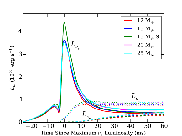
Figure 1.— Unoscillated energy luminosity as a function of time for all three main neutrino channels ($\nu_{e}$, $\bar{\nu}_{e}$, and $\nu_{x}$) for our five progenitor models. The solid line represents the $\nu_{e}$ energy luminosity, the dashed line represents the $\bar{\nu}_{e}$ luminosity, and the dot-dashed line represents the $\nu_{x}$ luminosity. “S” designates the Shen EOS while the rest of the models use the LSEOS with $K=220$ MeV. Shown is a cubic spline fit to the numerical data. Time is calculated since the peak of the $\nu_{e}$ luminosity. The $\nu_{x}$ luminosity is shown for the four neutrino types ($\nu_{\mu},\nu_{\tau},\bar{\nu}_{\mu}$, and $\bar{\nu}_{\tau}$). The luminosity for any one of these four neutrino types will be one-quarter of the value shown here for $\nu_{x}$.

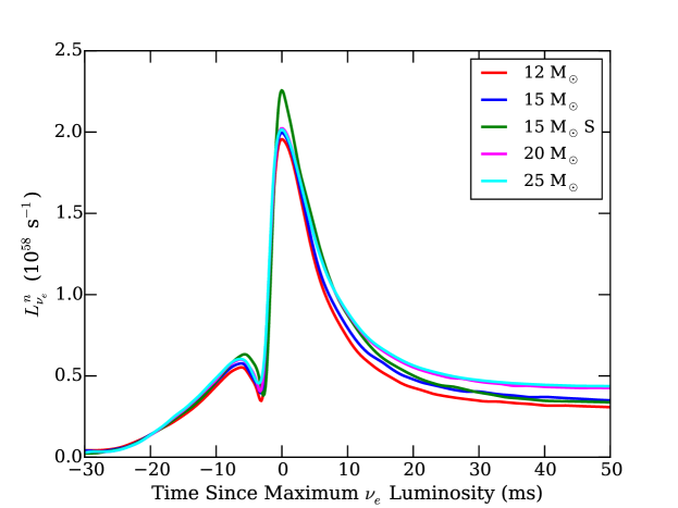
Figure 2.— Unoscillated $\nu_{e}$ number luminosity as a function of time over breakout for the various models. The “S” in the figure legend refers to the Shen EOS; the rest of the models use the LSEOS with $K=220$ MeV. The time is centered on the time of maximum $\nu_{e}$ luminosity. The luminosity shows two peaks: a small peak on the initial rise, and a large peak following a sharp rise. The first, smaller peak is due to neutrinos from the neutronization of the collapsing core; the second, larger peak is from $\nu_{e}$’s created by electron capture on free protons liberated by the shock.

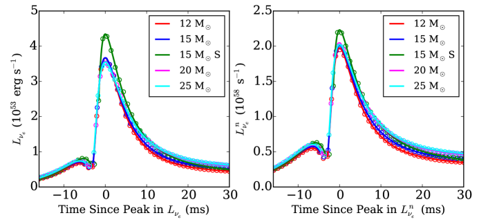
Figure 3.— Fits to the models, using Equations (1) and (2). Left: fits to the unoscillated energy luminosity. The parameters used in the fits are in Tables 3 and 5. Right: fits to the unoscillated number luminosity. The parameters used in these fits are in Tables 4 and 6. The numerical model data points are shown as circles, while the fits of Equations (1) and (2) are shown as lines. For each model, the local minimum between the preshock neutronization peak and the breakout burst peak is not well fit by either of Equations (1) and  (2), and so no attempt is made to fit it in this figure.

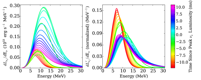
Figure 4.— Unoscillated energy spectra for the 15 $M_{\odot}$ LSEOS model for a range of times through the breakout burst. Left: the full, true spectra. Right: the normalized spectra, normalized so that the area under the normalized spectrum of each time (integrated over energy) is 1. Both panels show spectra over the same time range.

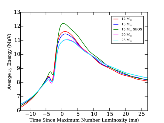
Figure 5.— Average $\nu_{e}$ energy as a function of time shown for all the models through the breakout burst. The average energy is defined by Equation (3). Time is calculated as time since maximum number luminosity for the fits to the number luminosity for each model. For the same EOS, the peak average energy decreases with progenitor mass down to 20 $M_{\odot}$, with the 20 and 25 $M_{\odot}$ progenitors showing comparable values, while the average energy in the tail after peak increases with progenitor mass (again, with the 20 and 25 $M_{\odot}$ progenitors showing comparable values). The models show a smaller peak in average energy, which is associated with the pre-breakout neutronization peak. The 15 $M_{\odot}$ Shen EOS model has a slightly higher average average energy during both the breakout burst peak and preshock neutronization peak compared to its LSEOS counterpart, but comparable average energy coming into and leaving the breakout burst. The average energy for all the models peaks at a time slightly after the time of maximum number luminosity.

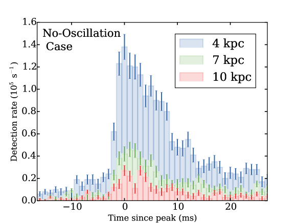
Figure 6.— Example realization of detection rates in the no-oscillation case with 1$\sigma$ error bars for CCSN neutrino detections in Hyper-K at distances of 4, 7, and 10 kpc, binned in 1 ms time bins. This figure not only shows the overall increase in signal expected in Hyper-K as the distance to the SN decreases but also gives a general sense of how the expected noise and error bars in each time bin depend on $D$.

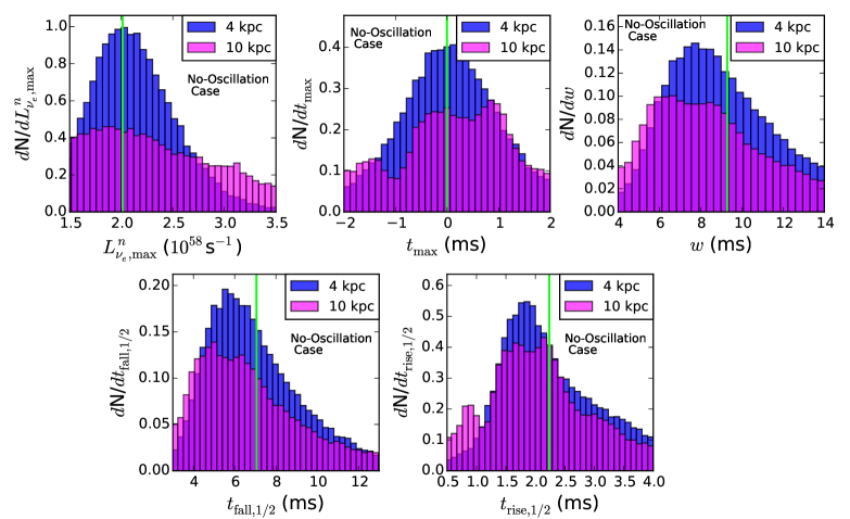
Figure 7.— PDFs for the physical parameters derived from fits of Equation (1) to the simulated observations for Super-K for the 15 $M_{\odot}$ LSEOS model in the no-oscillation case. For each parameter, blue shows the PDF corresponding to a supernova at a distance of 4 kpc and magenta shows the PDF corresponding to a supernova at a distance of 10 kpc. Overlap between the two PDFs is shown in purple. The model value is shown as a green vertical line.

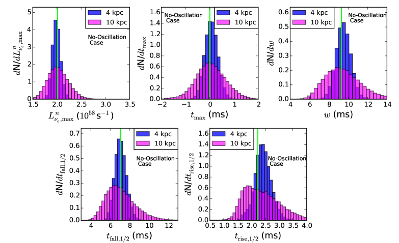
Figure 8.— Same as Figure 7, but for Hyper-K in the no-oscillation case.

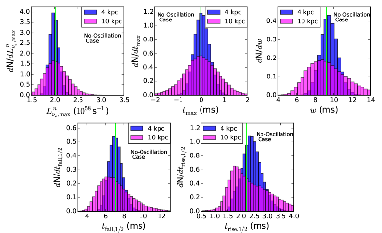
Figure 9.— Same as Figure 7, but for DUNE in the no-oscillation case.

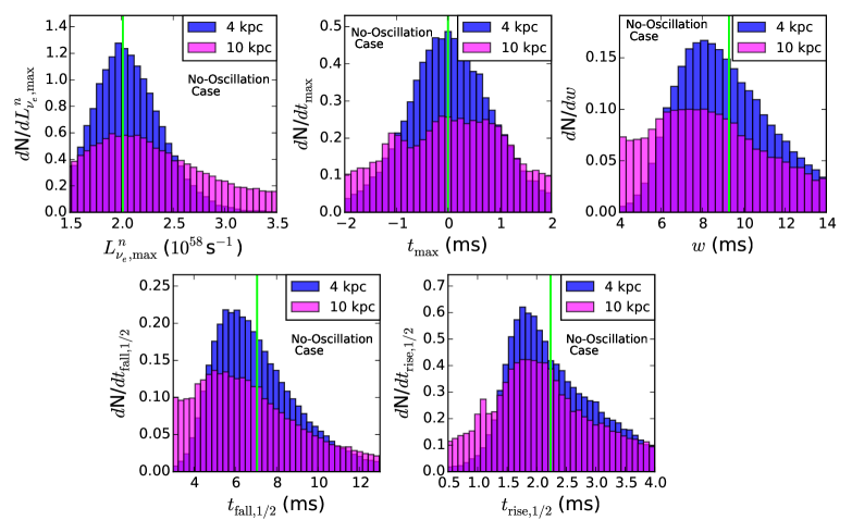
Figure 10.— Same as Figure 7, but for JUNO in the no-oscillation case.

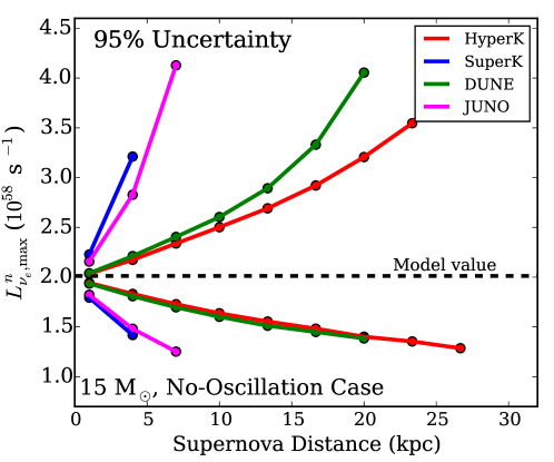
Figure 11.— The 95% uncertainty in measuring $L^{n}_{\nu_{e},\mathrm{max}}$ as a function of distance for various detectors for the 15 $M_{\odot}$ LSEOS model, in the no-oscillation case. For each detector, the lines represent the span needed to include 95% of the $L^{n}_{\nu_{e},\mathrm{max}}$’s calculated from the set of $5\times 10^{4}$ sampled observations. When the uncertainty values for a specific detector get either too large or too small relative to the model value, we stop plotting the uncertainty at that distance and greater distances. The uncertainty values for Super-K and JUNO were cut off at 7 kpc if the previous criteria were not met at 7 kpc because of the small number of events for an SN beyond that distance.

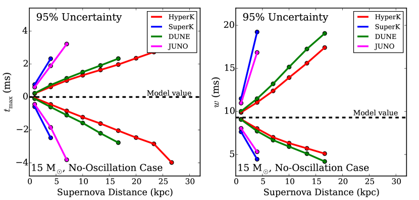
Figure 12.— Same as Figure 11, but for $t_{\mathrm{max}}$ (left) and $w$ (right), in the no-oscillation case.

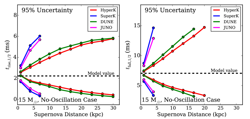
Figure 13.— Same as Figure 11, but for $t_{\mathrm{rise},\nobreak 1/2}$ (left) and $t_{\mathrm{fall},\nobreak 1/2}$ (right), in the no-oscillation case.

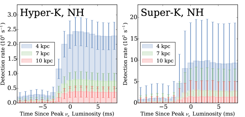
Figure 14.— For Hyper-K (left) and for Super-K (right), the expected light curve for SNe at 4, 7, and 10 kpc, incorporating the neutrino oscillations expected in the case of the NH. Detections of neutrinos of all flavors are taken into account, with IBDs and NC scattering off of oxygen subtracted, and (for JUNO) IBDs and NC scattering off of carbon subtracted. Each time bin shows the mean count rate in that time bin over 10⁴ realizations, and the error bars show the standard deviation based on the same 10⁴ realizations.

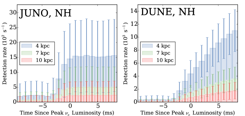
Figure 15.— Similar to Figure 14, but for JUNO (left) and DUNE (right). For JUNO, IBDs and NC scatterings off of carbon have been subtracted. For DUNE, no signals from any detection channel have been subtracted.

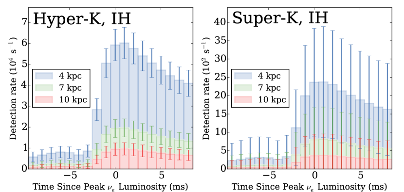
Figure 16.— Similar to Figure 14, but using the neutrino oscillations expected for the IH instead of the NH.

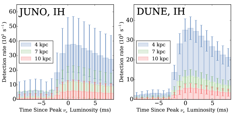
Figure 17.— Similar to Figure 15, but using the neutrino oscillations expected for the IH instead of the NH.

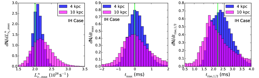
Figure 18.— Same as Figure 8, but for the IH case and with only $L^{n}_{\nu_{e},\mathrm{max}}$, $t_{\mathrm{max}}$, and $t_{\mathrm{rise},\nobreak 1/2}$ shown. For Hyper-K, the background signals due to IBDs and NC scatterings off of oxygen have been subtracted.

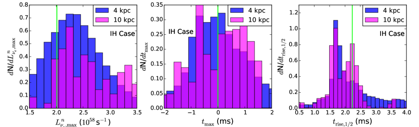
Figure 19.— Same as Figure 18, but for Super-K in the IH case. For Super-K, the background signals due to IBDs and NC scatterings off of oxygen have been subtracted.

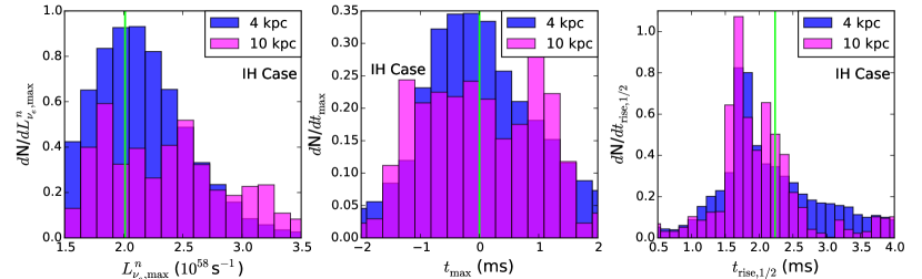
Figure 20.— Same as Figure 18, but for JUNO in the IH case. For JUNO, the background signals due to IBDs and NC scatterings off of carbon have been subtracted.

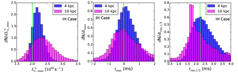
Figure 21.— Same as Figure 18, but for DUNE in the IH case. For DUNE, signals have been subtracted for any detection channel.

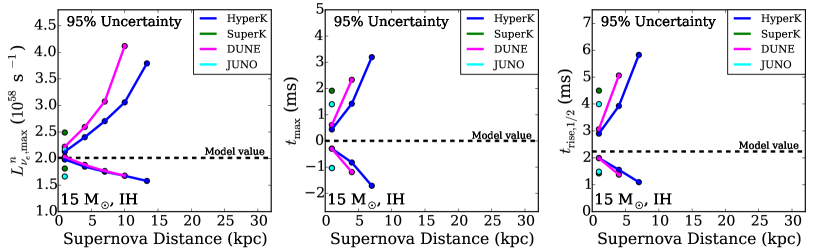
Figure 22.— Similar to Figure 11, but for $L^{n}_{\nu_{e},\mathrm{max}}$ (left), $t_{\mathrm{max}}$ (middle), and $t_{\mathrm{rise},\nobreak 1/2}$ (right), in the no-oscillation case. In all cases, the data for JUNO and/or Super-K are not plotted beyond 1 kpc, and the data are shown as a single point rather than a line connecting multiple points.

Figure A1.— The $\nu_{e}$ and $\bar{\nu}_{e}$ matter-interaction cross sections used in our study over the domain of neutrino energies relevant to our study. The ¹⁶O$(\bar{\nu}_{e},e^{+})$X cross section and both the ¹²C cross sections are not plotted to zero at low energies owing to a lack of tabulated data at these energy values from the sources used. The cross sections are assumed to be zero below the lowest extent of the tabulated data.

References

- Aartsen et al. (2013) Aartsen, M., Abbasi, R., Abdou, Y., et al. 2013, arXiv preprint arXiv:1309.7008
- Abbasi (2010) Abbasi, R. 2010, International Journal of Modern Physics D, 19, 1041
- Abbasi et al. (2011) Abbasi, R., Abdou, Y., Abu-Zayyad, T., et al. 2011, A&A, 535, A109
- Abe et al. (2011) Abe, K., Abe, T., Aihara, H., et al. 2011, arXiv preprint arXiv:1109.3262
- Abe et al. (2014) Abe, K., Adam, J., Aihara, H., et al. 2014, arXiv e-prints, arXiv:1407.7389
- Abe et al. (2008) Abe, S., Ebihara, T., Enomoto, S., et al. 2008, Physical Review Letters, 100, 221803
- Achterberg et al. (2006) Achterberg, A., Ackermann, M., Adams, J., et al. 2006, Astroparticle Physics, 26, 155
- Adams et al. (2013) Adams, S. M., Kochanek, C. S., Beacom, J. F., Vagins, M. R., & Stanek, K. Z. 2013, ApJ, 778, 164
- Aglietta et al. (1992) Aglietta, M., Alpat, B., Alyea, E., et al. 1992, Il Nuovo Cimento A Series 11, 105, 1793
- Ando & Sato (2002) Ando, S., & Sato, K. 2002, Progress of theoretical physics, 107, 957
- Antonioli et al. (2004) Antonioli, P., Fienberg, R. T., Fleurot, F., et al. 2004, New Journal of Physics, 6, 114
- Beacom et al. (2002) Beacom, J. F., Farr, W. M., & Vogel, P. 2002, Physical Review D, 66, 033001
- Beacom & Vagins (2004) Beacom, J. F., & Vagins, M. R. 2004, Physical review letters, 93, 171101
- Bellini et al. (2014) Bellini, G., Benziger, J., Bick, D., et al. 2014, Physical Review D, 89, 112007
- Bionta et al. (1987) Bionta, R., Blewitt, G., Bratton, C., et al. 1987, Physical Review Letters, 58, 1494
- Burrows & Lattimer (1986) Burrows, A., & Lattimer, J. M. 1986, ApJ, 307, 178
- Burrows & Mazurek (1983) Burrows, A., & Mazurek, T. L. 1983, Nature, 301, 315
- Burrows et al. (2006) Burrows, A., Reddy, S., & Thompson, T. A. 2006, Nuclear Physics A, 777, 356
- Eguchi et al. (2003) Eguchi, K., Enomoto, S., Furuno, K., et al. 2003, Physical Review Letters, 90, 021802
- Franco et al. (2011) Franco, D., Consolati, G., & Trezzi, D. 2011, Physical Review C, 83, 015504
- Fukuda et al. (2003) Fukuda, S., Fukuda, Y., Hayakawa, T., et al. 2003, Nuclear Instruments and Methods in Physics Research Section A: Accelerators, Spectrometers, Detectors and Associated Equipment, 501, 418
- Fukugita et al. (1988) Fukugita, M., Kohyama, Y., & Kubodera, K. 1988, Physics Letters B, 212, 139
- Goodman (2015) Goodman, M. 2015, Advances in High Energy Physics, 2015, 256351
- Halzen et al. (1996) Halzen, F., Jacobsen, J., & Zas, E. 1996, Physical Review D, 53, 7359
- Hirata et al. (1987) Hirata, K., Kajita, T., Koshiba, M., et al. 1987, Physical Review Letters, 58, 1490
- Ikeda et al. (2007) Ikeda, M., Takeda, A., Fukuda, Y., et al. 2007, ApJ, 669, 519
- Kachelrieß et al. (2005) Kachelrieß, M., Tomàs, R., Buras, R., et al. 2005, Phys. Rev. D, 71, 063003
- Kino et al. (2000) Kino, Y., Sekine, T., Sato, Y., et al. 2000, Journal of Nuclear and Radiochemical Sciences, 1, 63
- Kolbe et al. (2003) Kolbe, E., Langanke, K., Martinez-Pinedo, G., & Vogel, P. 2003, Journal of Physics G: Nuclear and Particle Physics, 29, 2569
- Kolbe et al. (1999) Kolbe, E., Langanke, K., & Vogel, P. 1999, Nuclear Physics A, 652, 91
- Kolbe et al. (2002) Kolbe, E., Langanke, K., & Vogel, P. 2002, Phys. Rev. D, 66, 013007
- Laha & Beacom (2014) Laha, R., & Beacom, J. F. 2014, Phys. Rev. D, 89, 063007
- Laha et al. (2014) Laha, R., Beacom, J. F., & Agarwalla, S. K. 2014, arXiv e-prints, arXiv:1412.8425
- Lattimer & Swesty (1991) Lattimer, J. M., & Swesty, F. D. 1991, Nuclear Physics A, 535, 331
- Li (2014) Li, Y.-F. 2014, International Journal of Modern Physics Conference Series, 31, 1460300
- Marciano & Parsa (2003) Marciano, W. J., & Parsa, Z. 2003, Journal of Physics G Nuclear Physics, 29, 2629
- Mirizzi et al. (2015) Mirizzi, A., Tamborra, I., Janka, H.-T., et al. 2015, arXiv preprint arXiv:1508.00785
- Mori et al. (2013) Mori, T., Collaboration, S.-K., et al. 2013, Nuclear Instruments and Methods in Physics Research Section A: Accelerators, Spectrometers, Detectors and Associated Equipment, 732, 316
- Oberauer et al. (2005) Oberauer, L., Von Feilitzsch, F., & Potzel, W. 2005, Nuclear Physics B-Proceedings Supplements, 138, 108
- Olive et al. (2014) Olive, K. A., Agashe, K., Amsler, C., et al. 2014, Chinese Physics C, 38, 090001
- Patterson (2013) Patterson, R. B. 2013, Nuclear Physics B Proceedings Supplements, 235, 151
- Pryor et al. (1988) Pryor, C., Roos, C. E., & Webster, M. S. 1988, The Astrophysical Journal, 329, 335
- Rubbia et al. (2011) Rubbia, C., Antonello, M., Aprili, P., et al. 2011, Journal of Instrumentation, 6, P07011
- Ryazhskaya & Ryasnyĭ (1992) Ryazhskaya, O., & Ryasnyĭ, V. 1992, ZhETF Pisma Redaktsiiu, 56, 433
- Scholberg (2008) Scholberg, K. 2008, Astronomische Nachrichten, 329, 337
- Sekiya (2013) Sekiya, H. 2013, arXiv e-prints, arXiv:1307.3686
- Shen et al. (1998a) Shen, H., Toki, H., Oyamatsu, K., & Sumiyoshi, K. 1998a, Nuclear Physics A, 637, 435
- Shen et al. (1998b) —. 1998b, Progress of Theoretical Physics, 100, 1013
- Sullivan et al. (2015) Sullivan, C., O’Connor, E., Zegers, R. G. T., Grubb, T., & Austin, S. M. 2015, arXiv e-prints, arXiv:1508.07348
- Tomàs et al. (2003) Tomàs, R., Semikoz, D., Raffelt, G. G., Kachelrieß, M., & Dighe, A. S. 2003, Phys. Rev. D, 68, 093013
- Vagins (2012) Vagins, M. R. 2012, Nuclear Physics B-Proceedings Supplements, 229, 325
- Watanabe et al. (2009) Watanabe, H., Zhang, H., Abe, K., et al. 2009, Astroparticle Physics, 31, 320
- Woosley & Heger (2007) Woosley, S. E., & Heger, A. 2007, Phys. Rep., 442, 269