Measuring the vertical age structure of the Galactic disc using asteroseismology and SAGA

Abstract

The existence of a vertical age gradient in the Milky Way disc has been indirectly known for long. Here, we measure it directly for the first time with seismic ages, using red giants observed by Kepler. We use Strömgren photometry to gauge the selection function of asteroseismic targets, and derive colour and magnitude limits where giants with measured oscillations are representative of the underlying population in the field. Limits in the 2MASS system are also derived. We lay out a method to assess and correct for target selection effects independent of Galaxy models. We find that low mass, i.e. old red giants dominate at increasing Galactic heights, whereas closer to the Galactic plane they exhibit a wide range of ages and metallicities. Parametrizing this as a vertical gradient returns approximately $4$ Gyr kpc^-1 for the disc we probe, although with a large dispersion of ages at all heights. The ages of stars show a smooth distribution over the last $\simeq 10$ Gyr, consistent with a mostly quiescent evolution for the Milky Way disc since a redshift of about 2. We also find a flat age-metallicity relation for disc stars. Finally, we show how to use secondary clump stars to estimate the present-day intrinsic metallicity spread, and suggest using their number count as a new proxy for tracing the aging of the disc. This work highlights the power of asteroseismology for Galactic studies; however, we also emphasize the need for better constraints on stellar mass-loss, which is a major source of systematic age uncertainties in red giant stars.

1 Introduction

A substantial fraction of the baryonic matter of the Milky Way is contained in its disc, where much of the evolutionary activity takes place. Thus, knowledge of disc properties is crucial for understanding how galaxies form and evolve. Late-type Milky Way-like galaxies are common in the local universe. However, we can at best measure integrated properties for external galaxies, while the Milky Way offers us the unique opportunity to study its individual baryonic components.

Star counts have revealed that the disc of the Milky Way is best described by two populations, one with shorter and one with longer scale-heights, dubbed the “thin” and the “thick” disc (e.g., Gilmore & Reid, 1983; Jurić et al., 2008). This double disc behaviour is also inferred from observations of edge-on galaxies, where the thick disc appears as a puffed up component extending to a larger height above a sharper thin disc (e.g., Burstein, 1979; van der Kruit & Searle, 1981; Yoachim & Dalcanton, 2006). Although it is usually possible to fit the vertical density/luminosity profile of late-type galaxies as a double-exponential profile, its interpretation is still a matter of debate. In particular, it is unclear if the thin and thick disc in the Milky Way are real, separated structural entities, or not (e.g., Norris, 1987; Nemec & Nemec, 1991; Schönrich & Binney, 2009b; Bovy et al., 2012). These different interpretations on disc’s decomposition underpin much of the theoretical framework for understanding its origin and evolution. Models in which the thick disc is formed at some point during the history of the Galaxy via an external mechanism (in particular accretion and/or mergers) best fit the picture in which the thin and the thick disc are real separated entities (e.g., Chiappini et al., 1997; Abadi et al., 2003; Brook et al., 2004; Villalobos & Helmi, 2008; Kazantzidis et al., 2008; Scannapieco et al., 2009). This scenario acquired momentum in the framework of cold dark matter models, where structures (and galaxies) in the universe form hierarchically (e.g., White & Rees, 1978; Searle & Zinn, 1978). Thus, the growth of a spiral galaxy over cosmic time would be responsible for puffing up the disc, also “heating” the kinematics of its stars. In contrast, internal dynamical evolution (primarily in the form of radial mixing e.g., Schönrich & Binney, 2009a, b; Loebman et al., 2011) favours the scenario in which the thick disc is the evolutionary end point of an initially pure thin disc, without requiring a heating mechanism. Internal sources of dynamical disc-heating, e.g. from giant molecular clouds or clump-induced stellar scattering, may also contribute to thick disc formation (e.g., Hänninen & Flynn, 2002; Bournaud et al., 2009). Although merger events can happen at early times, in this picture the formation of the Galaxy is mostly quiescent.

As is often the case, the real –yet unsolved– picture of galaxy formation is more complicated than the simplistic sketches drawn above. The latest numerical simulations indicate that hierarchical accretion occurring at early times can imprint a signature of hot kinematic and roundish structures. Other processes then factor into the following more quiescent phases, characterized by the formation of younger disc stars in a more flattened, rotationally supported configuration (e.g., Genzel et al., 2006; Bournaud et al., 2009; Aumer et al., 2010; House et al., 2011; Forbes et al., 2012; Stinson et al., 2013; Bird et al., 2013). Importantly, high-redshift observations suggest that, for galaxies in the Milky Way mass range, this might not happen in an inside-out fashion (van Dokkum et al., 2013).

Historically, the study of chemical and kinematic properties of stars in the (rather local) disc, has been used to shed light on these different formation scenarios. Thin disc stars are observed to be on average more metal-rich and less alpha-enhanced than thick disc stars (e.g., Edvardsson et al., 1993; Chen et al., 2000; Reddy et al., 2003; Fuhrmann, 2008; Bensby et al., 2014). Due to stellar evolutionary timescales the enrichment in alpha elements happens relatively quickly (e.g. Tinsley, 1979; Matteucci & Greggio, 1986). Thus, for the bulk of local disc stars it is customary to interpret this chemical distinction into an age difference (but see Chiappini et al. 2015 and Martig et al. 2015 for the possible existence of local outliers). In this picture the thick disc would be the result of some event in the history of the early Galaxy and thus metal-poor and alpha-enhanced. This interpretation however has been recently challenged by the observational evidence that alpha-enhanced thick disc stars may also extend to super-solar metallicities (e.g., Feltzing & Bensby, 2008; Casagrande et al., 2011; Trevisan et al., 2011; Bensby et al., 2014). This can be explained if –at least some of– the thick disc is composed of stars originating from the inner Galaxy, where the chemical enrichment happened faster. In terms of kinematics, thin disc stars are cooler (i.e. with smaller vertical velocity with respect to the Galactic plane) and have higher Galactic rotational velocity compared to thick disc stars then referred to as kinematically hot. Low rotational velocities (due to larger asymmetric drift) imply higher velocity dispersion for thick disc stars, which then point to older ages, either born hot or heated up. In fact, the age-velocity dispersion relation has long been known to indicate the existence of a vertical age gradient (e.g. von Hoerner, 1960; Mayor, 1974; Wielen, 1977; Holmberg et al., 2007): its direct measurement is the subject of the present study.

The dissection of disc components based only on chemistry and kinematic is far from trivial (e.g., Schönrich & Binney, 2009b). In this context, stellar ages are expected to provide an additional powerful criterion. Also, age cohorts are easier to compare with numerical simulations than chemistry based investigations, bypassing uncertainties related to the implementation of the chemistry in the models. From the observational point of view however, even when accurate astrometric distances are available to allow comparison of stars with isochrones, the derived ages are still highly uncertain, and statistical techniques are required to avoid biases (e.g., Pont & Eyer, 2004; Jørgensen & Lindegren, 2005; Serenelli et al., 2013). Furthermore, isochrone dating is meaningful only for stars in the turnoff and subgiant phase, where stars of different ages are clearly separated on the H-R diagram. This is in contrast, for example, to stars on the red giant branch, where isochrones with vastly different ages can fit observational data such as effective temperatures, metallicities, and surface gravities equally well within their errors. As a result, so far the derivation of stellar ages has been essentially limited to main-sequence F and G type stars with Hipparcos parallaxes, i.e. around $\sim 100$ pc from the Sun (e.g., Feltzing et al., 2001; Bensby et al., 2003; Nordström et al., 2004; Haywood, 2008; Casagrande et al., 2011). All these studies agree on the fact that the thick disc is older than the thin disc. Yet, only a minor fraction of stars in the solar neighbourhood belong to the thick disc.

It is now possible to break this impasse thanks to asteroseismology. In particular, the latest spaceborne missions such as CoRoT (Baglin & Fridlund, 2006) and Kepler/K2 (Gilliland et al., 2010; Howell et al., 2014) allow us to robustly measure global oscillation frequencies in several thousands of stars, in particular red giants, which in turn make it possible to determine fundamental physical quantities, including radii, distances and masses. Most importantly, once a star has evolved to the red giant phase, its age is determined to good approximation by the time spent in the core-hydrogen burning phase, and this is predominantly a function of the stellar mass. Although mass-loss can partly clutter this relationship, as we will discuss later in the paper, to first approximation the mass of a red giant is a proxy for its age. In addition, because of the intrinsic luminosity of red giants, they can easily be used to probe distances up to a few kpc (e.g. Miglio et al., 2013b).

This has profound impact for Milky Way studies, and in fact synergy with asteroseismology is now sought by all major surveys in stellar and Galactic archaeology (e.g. Pinsonneault et al., 2014; De Silva et al., 2015). With similar motivation, we have started the Strömgren survey for Asteroseismology and Galactic Archaeology (SAGA, Casagrande et al., 2014, hereafter Paper I) which so far has derived classic and asteroseismic stellar parameters for nearly 1000 red giants with measured seismic oscillations in the Kepler field. In this paper we derive stellar ages for the entire SAGA asteroseismic sample, and use them to study the vertical age structure of the Milky Way disc. Our novel approach uses the power of seismology to address thorny issues in Galactic evolution, such as the age-metallicity relation, and to provide in situ measurements of stellar ages at different heights above the Galactic plane, at the transition between the thin and the thick disc. The study of the vertical metallicity structure of the disc with SAGA will be presented in a companion paper by Schlesinger et al. (2015).

The paper is organized as follows: in Section 2 we review the SAGA survey, and present the derivation of stellar ages for the seismic sample. In Section 3 we investigate the selection function of the Kepler satellite, and identify the colour and magnitude intervals within which the asteroseismic sample is representative of the underlying stellar population in the field. This allows us to define clear selection criteria, which are then used in Section 4 to derive vertical mass and age gradients. We provide raw gradients, i.e. obtained by simply fitting all stars that pass the selection criteria in Section 4.2. The biases introduced by our target selection criteria are also assessed, and gradients corrected for these effects are presented in Section 4.3. The implications of the age-metallicity relation, and of the age distribution of red giants to constrain the evolution of the Galactic disc are discussed in Section 5. In Section 6 we suggest using secondary clump stars as age candles for Galactic Archaeology. Finally, we conclude in Section 7.

2 The SAGA

The purpose of the SAGA is to uniformly and homogeneously observe stars in the Strömgren $uvby$ system across the Kepler field, in order to transform it into a new benchmark for Galactic studies, similar to the solar neighbourhood. Details on survey rationale, strategy, observations and data reduction are provided in Paper I, and here we briefly summarize the information relevant for the present work. So far, observations of a stripe centred at Galactic longitude $l\simeq 74^{\circ}$ and covering latitude $8^{\circ}\lesssim b\lesssim 20^{\circ}$ have been reduced and analyzed. This geometry is particularly well suited to study vertical gradients in the Galactic disc.

The Strömgren $uvby$ system (Strömgren, 1963) was designed for the determination of basic stellar parameters (see e.g., Árnadóttir et al., 2010, and references therein). Its $y$ magnitudes are defined to be essentially the same as the Johnson $V$ (e.g., Bessell, 2005), and in this work we will refer to the two interchangeably.

SAGA observations are conducted with the Wide Field Camera on the $2.5$-m Isaac Newton Telescope (INT), which in virtue of its large field of view and pixel size is ideal for wide field optical imaging surveys. The purpose of our survey is to obtain good photometry for all stars in the magnitude range $10\lesssim y\lesssim 14$, where most targets were selected to measure oscillations with Kepler. This requirement can be easily achieved with short exposures on a $2.5$-m telescope; indeed, all stars for which Kepler measured oscillations are essentially detected in our survey (with a completeness $\gtrsim 95$ per cent, see Paper I). SAGA is magnitude complete to about $y\simeq 16$ mag, thus providing an unbiased, magnitude-limited census of stars in the Galactic stripe observed. Stars are still detected at fainter magnitudes ($y\lesssim 18$), although with increasingly larger photometric errors and incompleteness, totalling some $29,000$ objects in the stripe observed so far. Thus, we can build two samples from our observations. First, a magnitude complete and unbiased photometric sample down to $y\simeq 16$ mag, which we refer to as the full photometric catalog. Second, we extract a subset of 989 stars which have oscillations measured by Kepler, dubbed the asteroseismic catalog. Note that the stars for which Kepler measured oscillations were selected in a non trivial way. By comparing the properties of the asteroseismic and full photometric catalogs we can assess the Kepler selection function (Section 3).

Before addressing the Kepler selection function, we briefly recall the salient features of the full photometric and asteroseismic catalog. For the asteroseismic catalog we also derive stellar ages, and discuss their precision.

2.1 Full photometric sample

The full photometric catalog provides $uvby$ photometry for several thousands of stellar sources down to a magnitude completeness limit of $y\simeq 16$. The asteroseismic catalog is a subset of the targets in the full photometric catalog, and thus the data reduction and analysis is identical for all stars in SAGA. In this work, for both the asteroseismic and the full photometric sample (or any sub-sample extracted from them) we use only stars with reliable photometry in all $uvby$ bands (Pflg=0 flag, see also figure 4 in Paper I). This requirement excludes stars whose errors are larger than the ridge-lines defined by the bulk of photometric errors, as customarily done in photometric analysis, and does not introduce any bias for our purposes. Furthermore, we have verified that the fraction of stars excluded as a function of increasing $y$ mag is nearly identical for both the asteroseismic and the full photometric sample. This is true for the two samples as a whole, or when restricting them only to giants. A flag also identifies stars with reliable $\rm{[Fe/H]}$, i.e. those objects for which the Strömgren metallicity calibration is used within its range of applicability (Mflg=0). This flag automatically excludes stars with $\rm{[Fe/H]}\geqslant 0.5$, where such high values could be the result of extrapolations in the metallicity calibration and/or stem from photometric and reddening errors. Again, this limit is not expected to introduce any bias given the paucity (or even the non-existence, see e.g., Taylor 2006) of star more metal-rich than $0.5$ dex in nature (i.e. those present in our catalog are likely flawed). Later in the paper, we will use only stars with both Pflg and Mflg equal to zero to constrain the Kepler selection function and to study the vertical stellar mass and age struture in the Galactic disc.

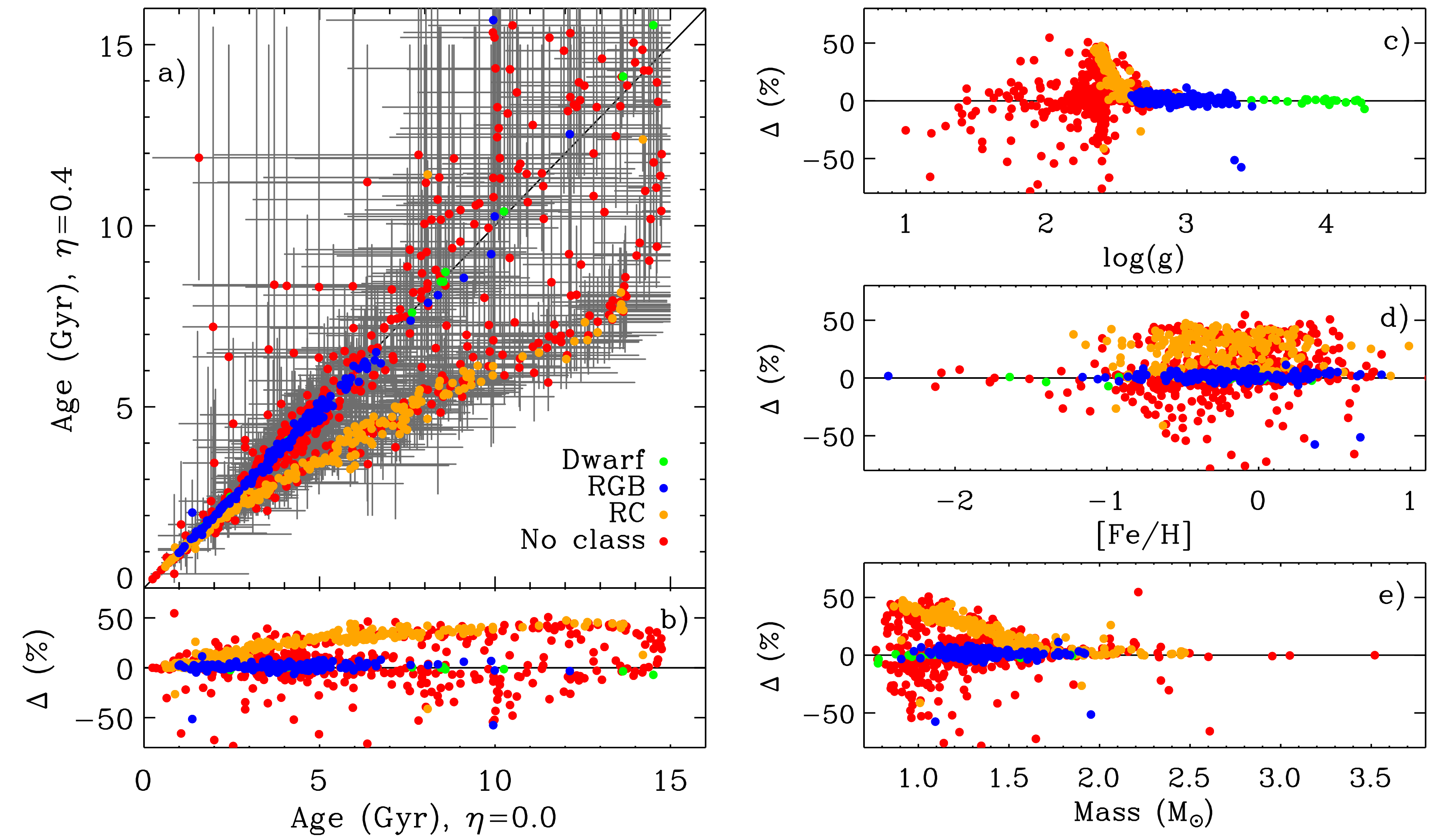
Figure 1: Panel a): comparison between ages obtained with mass-loss (vertical axis, $\eta=0.4$), and without mass-loss (horizontal axis). Colours identify stars with different seismic classification, as labelled (see also Paper I). Error bars are formal uncertainties, only. Panel b) to e): same as above, but showing the fractional age difference as function of different parameters.

2.2 Asteroseismic sample

The SAGA asteroseismic catalog consists of 989 stars identified by cross-matching our Strömgren observations with the dwarf sample of Chaplin et al. (2014) and the $\simeq 15,000$ giants from the Kepler Asteroseismic Science Consortium (KASC, Stello et al. 2013; Huber et al. 2014). Within SAGA, a novel approach is developed to couple classic and asteroseismic stellar parameters: for each target, the photometric effective temperature and metallicity, together with the asteroseismic mass, radius, surface gravity, mean density and distance are computed (Casagrande et al., 2010, 2014; Silva Aguirre et al., 2011, 2012). A detailed assessment of the uncertainties in these parameters is given in Paper I. For a large fraction of objects, evolutionary phase classification identifies whether a star is a dwarf (labelled as “Dwarf”, 23 such stars in our sample), is evolving along the red giant branch (“RGB”) or is already in the clump phase (“RC”). It was possible to robustly distinguish between the last two evolutionary phases for 427 stars, whereas for the remaining giants no classification is available (“NO”). In this paper, we refer to all stars classified as “RGB”, “RC”, or “NO” as red giants.

2.3 Asteroseismic ages

With the information available for each asteroseismic target it is rather straightforward to compute stellar properties. As described in Paper I, we apply a Bayesian scheme to sets of BaSTI isochrones (Pietrinferni et al., 2004, 2006). Flat priors are assumed for ages and metallicities over the entire grid of BaSTI models, meaning that at all ages, all metallicities are equally possible. A Salpeter (1955) Initial Mass Function (IMF, $\alpha=-2.35$) is also used (see details in Silva Aguirre et al., 2015). The adopted asteroseismic stellar parameters are derived using non-canonical BaSTI models with no mass-loss, but we explore the effect of varying some of the BaSTI prescriptions as described further below. As input parameters we consider the two global asteroseismic parameters $\Delta\nu$ and $\nu_{\mathrm{max}}$ and the atmospheric observables $T_{\rm{eff}}$ and $\rm{[Fe/H]}$. The information on the evolutionary phase (“RGB”, “RC”) is included as a prior when available, otherwise the probability that a star belongs to a given evolutionary status is determined by the input observables, the adopted IMF and the evolutionary timescales. The median and 68 per cent confidence levels of the probability distribution function determine the central value and (asymmetric) uncertainty of ages, which following the terminology of Paper I we refer to as formal uncertainties.

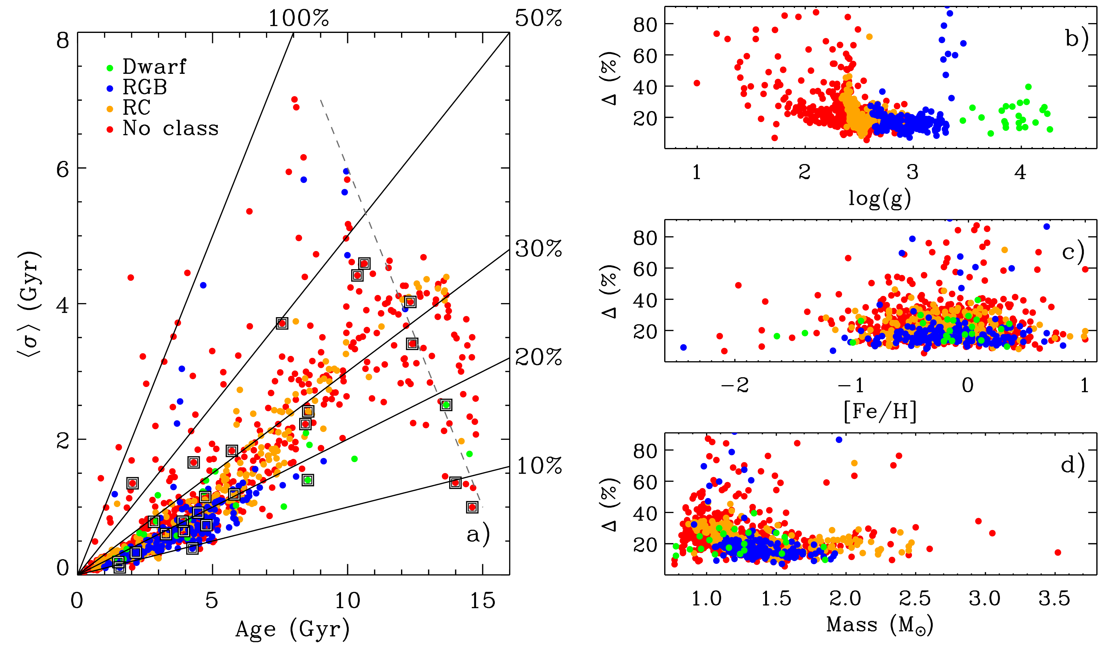
Figure 2: Panel a): final global age uncertainties $\langle\sigma\rangle$ (as defined in the text) for stars with different seismic classification plotted as function of their ages. Squares highlight stars with $\rm{[Fe/H]}<-1$, whereas continuous ridge-lines mark uncertainties between 10 and 100 per cent. Dashed line is the maximum uncertainty formally possible at old ages because of the sharp cut imposed at 15 Gyr. Panel b) to d): fractional age uncertainties as function of different parameters.

Overshooting in the main-sequence phase can significantly change the turn-off age of a star and is therefore important for our purposes. In order to assess its impact, in the present analysis we explore the effect of using BaSTI isochrones computed from stellar models not accounting for core convective overshoot during the central H-burning stage (dubbed canonical) as well as isochrones based on models including this effect (dubbed non-canonical, and adopted as reference). We note that all sets of BaSTI isochrones take into account semiconvection during the core helium-burning phase. The BaSTI theoretical framework for mass-loss implements the recipe of Reimers (1975):

$$\frac{dM}{dt}=\eta\,4\times 10^{-13}\frac{L}{gR}\,\left[\frac{\rm M_{\odot}}{{\rm yr}}\right]\,,$$ (1)

where $\eta$ is a (free) efficiency parameter that needs to be constrained by observations (see e.g. the recent analyses by McDonald & Zijlstra, 2015; Heyl et al., 2015). As we discuss further below, mass-loss efficiency can have a considerable impact on the parameters relevant for the present analysis. Sets of BaSTI stellar models have been computed for different values of $\eta$; we explore its effects by using the no mass-loss isochrones ($\eta=0$) as our reference set and compare to the stellar properties derived with the $\eta=0.4$ set.

As we did for the other seismic parameters, we pay particular attention to derive realistic uncertainties for our age estimates. The computation of ages for red giant stars heavily rely on the knowledge of their masses. Here, the mass of a star is essentially fit (with a grid-based Bayesian scheme) using scaling relations based on the observed $\Delta\nu$ and $\nu_{\rm{max}}$, and thus the mass is rather independent of the models adopted. Paper I demonstrated that for most stellar parameters, assuming a very efficient mass-loss ($\eta=0.4$) or neglecting core overshooting during the H-core burning phase affects the results significantly less than the formal uncertainty of the property under consideration. The same, however, does not hold for ages. Although the mass of a red giant is a useful proxy for age, it is important to distinguish between the initial mass which sets the evolutionary lifetime of a star, and the present-day (i.e. actual) stellar mass, which is derived from seismology. Thus, when inferring an age using the actual stellar mass, the value derived will depend on the past history of the star, whether or not significant mass-loss has occurred during its evolution.

There are very few observational constraints on mass-loss. Open clusters in the Kepler field suggest a value of $\eta$ between $0.1$ and $0.3$ (Miglio et al., 2012) for solar metallicity stars of masses $\sim$1.2–1.5 $\rm M_{\odot}$; observations of globular clusters reveal that mass-loss seems to be episodic and increasingly important when ascending the red giant branch (see e.g., Origlia et al., 2014), with recent studies suggesting a very inefficient mass-loss during this phase (Heyl et al., 2015). For the asteroseismic sample we also derive ages using BaSTI isochrones with $\eta=0.4$. This value corresponds to an efficient mass-loss process, and it is often used e.g., to reproduce the mean colours of horizontal branch stars in Galactic globular clusters, although this morphological feature is affected by other, also poorly constrained, parameters (e.g., Catelan, 2009; Gratton et al., 2010; Milone et al., 2014). By deriving ages with both $\eta=0$ and $0.4$, we can compare two extreme cases and derive a conservative estimate of the age uncertainty introduced by mass-loss.

The comparison of ages derived with and without mass-loss is done in Figure 1. Ages of dwarf stars are obviously unaffected by mass-loss, and the same conclusion holds for stars with “RGB” classification. It must be noticed that the distinction between “RGB” and “RC” is based on the average spacing between mixed dipole modes, and this measurement largely depends on the frequency resolution which smoothes over the spacing (e.g., Bedding et al., 2011). A clear identification of “RGB” stars is thus possible for $\log g\gtrsim 2.6$ i.e. on the lower part of the giant branch, where mass-loss turns out to be of little or no importance in the Reimers’ formulation. This explains the weak dependence of “RGB” ages on mass-loss. The effect of mass-loss increases when moving to lower gravities, and it is most dramatic for stars in the clump phase.

Isochrones including mass-loss return younger ages than those without mass-loss; this can be easily understood since a given mass –seismically inferred– will correspond to a higher initial mass in case of mass-loss, and thus evolve faster to its presently observed value. From Equation 1 it can be seen that the rate of mass-loss has an inverse dependence on mass. This implies a decreasing importance of mass-loss for increasing stellar mass. This is evident in Figure 1e, where only masses below about $1.7M_{\odot}$ are significantly affected by mass-loss. The fractional differences shown in Figure 1 deserve an obvious -yet important- word of caution. We define the reference ages as those without mass-loss. Within this context, a fractional difference of e.g., 50 per cent means that age estimates decrease by half when we factor in mass-loss. Should the same difference be computed using $\eta=0.4$ as reference, ages from mass-loss should then be increased by twice, implying a 100 per cent change in this example.

In addition to mass-loss, we have also tested the effect of canonical and non-canonical models (for a given $\eta$). The difference is negligible above 3 Gyr, with differences of a few per cent or less, while at younger ages (i.e. for masses above $\simeq 1.4M_{\odot}$) the effect can amount to a few hundreds Myr, thus translating in age differences of few tens of per cent for the youngest stars. The reason for this is that in this mass range, the inclusion of overshooting in the main-sequence phase plays a significant role in the turn-off age. Although part of this difference is compensated by a quicker evolution in the subgiant phase for stars with smaller helium cores (i.e. with no overshooting, see Maeder, 1974), the effect remains in more advanced stages.

To determine our final and global uncertainties on ages we adopt the same procedure used for other seismic parameters, but also account for the uncertainties related to mass-loss and the use of (non)-canonical models (see Paper I for details on the GARSTEC grid and Monte-Carlo approach discussed below). Briefly, we add quadratically to the formal asymmetric uncertainties obtained from our $\eta=0$ non-canonical BaSTI reference models half the difference between these results and the ones obtained with i) the GARSTEC grid, ii) the Monte-Carlo approach, iii) implementing mass-loss with $\eta=0.4$ and iv) using BaSTI canonical models. In most cases the uncertainties listed in i) to iv) dominate over the asymmetric formal uncertainty. For plotting purposes we use $\langle\sigma\rangle$ defined as the average of the (absolute) value of the upper and lower age uncertainty. Figure 2 shows both the absolute and relative age uncertainty of each star in our sample, along with their dependence on $\log g,\rm{[Fe/H]}$ and mass.

For most of the stars, the age uncertainty is between 10 and 30 per cent. When restricting to gravities higher than $\log g\simeq 2.6$, uncertainties of order 20 per cent are common. The lower part of the red giant branch is where the effect of mass-loss is weak for stars ascending it, and where seismic classification is able to separate “RGB” from “RC” stars. There is only a handful of “RGB” stars with uncertainties larger than about 30 per cent: those are located at the base of the red giant branch and have $\Delta\nu$, but not $\nu_{\rm{max}}$ measurements, explaining their larger errors. For dwarfs, our age uncertainties are also consistent with the results of Chaplin et al. (2014), who found a median age uncertainty of 25 per cent when having good constraints on $T_{\rm{eff}}$ and $\rm{[Fe/H]}$. For the 20 dwarfs we have in common with that work, which span an interval of about 10 Gyr, the mean age difference is 1 Gyr with a scatter of 3 Gyr. The largest differences occour for the most metal-poor stars, and the stars having Pflg and Mflg different from zero. These discrepancies likely arise from Chaplin et al. (2014) assuming a constant $\rm{[Fe/H]}=-0.2$ for all targets, but also our flagged stars might have less reliable metallicities.

At the oldest ages, formal uncertainties decrease because of the cut imposed at 15 Gyr (this is true for the upper uncertainty on ages, but obviously also the average $\langle\sigma\rangle$ is affected, see Figure 2). Notice that our global uncertainties (which include the effect of different models and mass-loss assumptions) partly blur this limit. We also remark that the accuracy of asteroseismic masses (and thus ages) obtained from scaling relations is still largely unexplored, especially in giants (see e.g., Miglio et al., 2013a). There are also indications that in the metal-poor regime ($\rm{[Fe/H]}\lesssim-1$) scaling relations might overestimate stellar masses by $15-20$ per cent (Epstein et al., 2014), thus returning ages systematically younger by more than 60 per cent (see e.g., Jendreieck et al., 2012). In absence of a more definitive assessments on the limits of the scaling relations, this source of uncertainty has not been included in our error budget. Our metal-poor stars are highlighted in Figure 2, and they cover the entire age range (i.e. we do also have metal-poor old stars) with formal uncertainties between 20 and 30 per cent (should scaling relations for metal-poor stars be trusted).

2.3.1 Asteroseismic ages: reality check

As for the other seismic parameters in Paper I, the solar-metallicity open cluster NGC 6819 offers an important benchmark to check our results. In Figure 3 we show the age distribution of its cluster members, from using all seismic members (Stello et al., 2011) to only a subset of them with the best Strömgren photometry and seismic evolutionary phase classification. We recall that for each star belonging to the cluster, we use its own metallicity rather than imposing the mean cluster $\rm{[Fe/H]}$ for all its members. Requiring good Mflg and Pflg does not seem to reduce the scatter, and thus improve the quality of the ages. This is partly expected: although our Bayesian scheme fits a number of observables, the main factor in determining ages is the stellar mass, which is mostly constrained by the asteroseismic observables. More crucial in improving the age precision is to select “RGB” stars only, from which we derive a mean (and median) age of $2.0\pm 0.2$ Gyr for this cluster. Essentially the same age, but with larger uncertainty, is obtained using other samples, as shown in Figure 3. Although somewhat on the young side, our age for NGC 6819 is in good agreement with a number of other age determinations based on colour-magnitude diagram fitting (e.g., Rosvick & Vandenberg, 1998; Kalirai et al., 2001; Yang et al., 2013), seismic masses (Basu et al., 2011), white dwarf cooling sequence (Bedin et al., 2015) and eclipsing binaries (Sandquist et al., 2013; Jeffries et al., 2013). Values in the literature range from $2.0$ to $2.7$ Gyr. Part of these differences depends on the models used in each study, as well as on the reddening and metallicity adopted for the cluster. We remark though the nearly perfect agreement with the age of $2.25\pm 0.20$ Gyr from the white dwarf cooling sequence and $2.25\pm 0.3$ Gyr from the main-sequence turn-off match when using the same BaSTI models (Bedin et al., 2015).

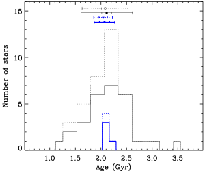
Figure 3: Age histogram for radial-velocity single members of the open cluster NGC 6819, selected according to the seismic membership of Stello et al. 2011. Thin black dotted line indicates all stars belonging to the cluster, without any further pruning. Thin continuous black line is when restricting the sample to stars with good Mflg and Pflg. Thick blue lines (dotted and continuous) are when further restricting to “RGB” stars. Circles in the upper part of the plot identify the mean value of each histogram, together with its standard deviation (outer bar) and the standard deviation of the mean (inner bar).

Moving to the entire asteroseismic sample, Figure 4 shows the age distribution of all stars, which peaks between 2 and 4 Gyr. While this distribution is not a proof of the reliability of the ages in itself, the ability to single out a population of “known” ages is. Such a population is provided by secondary clump stars, which are bound to be young ($\lesssim 2$ Gyr, see e.g. Girardi, 1999, and also Section 6 for the use of secondary clump stars as standard age candles).

The distribution in Figure 4 varies quite considerably when split according to seismic classification, shown on the right-hand panels. While the “RGB” sample clusters at young ages, “RC” stars peak around 2 Gyr with a tail at older ages. The age distribution of stars without seismic classification (which includes clump, upper and lower red giant branch, and asymptotic giant branch stars) is a mix of the two previous distributions characterized by a somewhat thicker tail at old ages. The lowest right-hand panel in Figure 4 shows ages for “RC” stars, sorted into the primary or secondary clump phase. It is important to stress that the distinction between primary and secondary clump stars is done here with a (rather arbitrary) cut at $\log g=2.5$. Thus, there is a certain level of contamination between the two phases, which surely broads the age distribution of plausibly secondary clump stars. In addition there is also contamination from members of NGC 6819 which peaks around 2 Gyr. Once the seismic members of the cluster are excluded, the typical age of secondary clump stars shifts to younger values, in accordance with expectations (e.g., Girardi, 1999), providing futher confidence on our asteroseismic ages. Should the same figure be done using ages derived with mass-loss, the overall distributions would remain quite similar, but the tail at older ages would be reduced, in particular for “RC” stars.

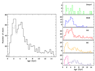
Figure 4: Age distribution of the entire asteroseismic sample (central panel), and when splitting stars according to seismic classification (right-hand side panels). The lowest right panel is the age distribution of stars having certain “RC” classification and sorted into primary (blue) and secondary (pink) clump according to their $\log g$ (see description in the text). Dotted lines are same distributions once members of the cluster NGC 6819 are excluded.

The above comparisons tell us that despite the various uncertainties associated with age determinations, our results are meaningful. On an absolute scale, the age we derive for the open cluster NGC 6819 is in agreement with the values reported in literature using a number of different methods. This holds at the metallicity of this cluster, which nevertheless is representative of the typical metallicity of most stars in the Kepler field. On a differential scale, once “RC” stars are identified as primary or secondary, they show different age distributions. Despite our rough $\log g$ criterium might partly blur this difference, the ability to recover the presence of young secondary clump stars gives us further trust on our ages.

3 Statistical properties of the asteroseismic sample

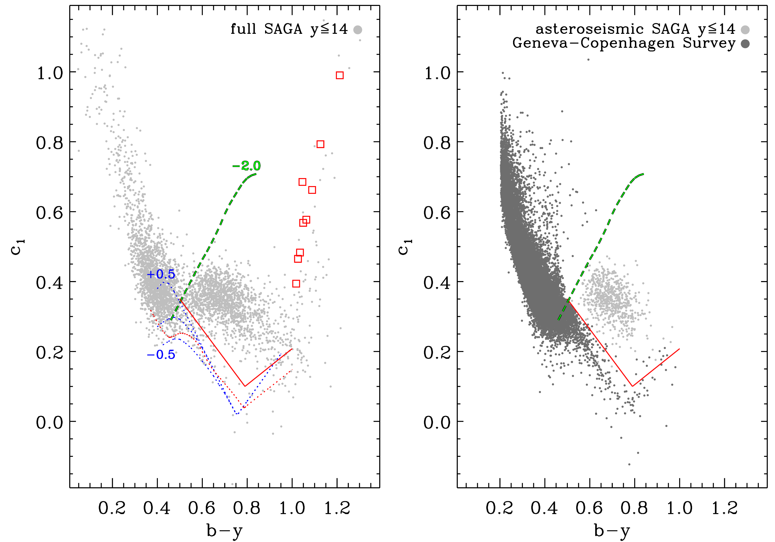
Figure 5: Left panel: $b-y$ vs. $c_{1}$ plane for the entire SAGA photometric catalog with $y\leq 14$ and Pflg=0. Dotted red line is the main-sequence fiducial of Olsen 1984, while the continuous red line is the $+0.06$ mag shift we use to separate dwarfs from giants. Open squares are cool M giants, also from Olsen 1984. For reference, the metallicity dependent dwarf sequences of Árnadóttir et al. 2010 are also shown (in blue, for $-0.5\leq\rm{[Fe/H]}\leq 0.5$ as indicated), as well as the metal-poor ($\rm{[Fe/H]}=-2.0$) red giant branch sequence of Anthony-Twarog & Twarog 1994. Right panel: dark gray circles identify all dwarf/subgiant stars in the Geneva-Copenhangen Survey, most of the late-type ones being succesfully delimited by our shifted fiducial (in red). Pale gray circles are all asteroseismic giants having good photometric and metallicity flags and $y\leq 14$.

In order to use our sample for investigating age and metallicity gradients in the Galactic disc, we need to know how stars with different properties are preferentially, or not, observed by the Kepler satellite. In other words, we need to know the Kepler selection function.

The selection criteria of the satellite were designed to optimize the scientific yield of the mission with regard to the detection of Earth-size planets in the habitable zone of cool main-sequence stars (Batalha et al., 2010). Even so, deriving the selection function for exoplanetary studies is far from trival (Petigura et al., 2013; Christiansen et al., 2014). For the sake of asteroseismic studies, entries in the KASC sample of giants (c.f. with Section 2.2) are based on a number of heterogeneous criteria (Huber et al., 2010; Pinsonneault et al., 2014). Fortunately, the full Strömgren catalog offers a way of assessing whether seismic giants with particular stellar properties are more likely (or not) to be observed by the Kepler satellite.

3.1 Constraining the Kepler selection function

Stellar oscillations cover a large range of timescales; for solar-like oscillations –as we are interested here– these range from a few minutes in dwarfs (cf e.g., with 5 minutes in the Sun, Leighton et al., 1962) to several days or more for the most luminous red giants (e.g., De Ridder et al., 2009; Dupret et al., 2009). The Kepler satellite has two observing modes: short-cadence (one minute), for dwarfs and subgiants (a little over 500 objects with measured oscillations in the Kepler field, see Chaplin et al., 2011, 2014) and long-cadence (thirty minutes) well suited for detecting oscillations in red giants.

With the exception of a few hundreds of dwarfs, most of the stars for which Kepler measured oscillations are giants. In order to assess how well these stars represent the underlying stellar population of giants, we use the full photometric catalog to build an unbiased sample of giants with well-defined magnitude and colour cuts. This task is facilitated both by the relatively bright magnitude limit we are probing, meaning that within a colour range most late-type stars are indeed giants, as well as by the fact that Strömgren colours offer a very powerful way to discriminate between cool dwarfs and giants. We use the $(b-y)$ vs. $c_{1}$ plane, which due to its sensitivity to $T_{\rm{eff}}$ and $\log g$ (in the relevant regions), can be regarded as the observational counterpart of an H-R diagram (e.g., Crawford, 1975; Olsen, 1984; Schuster et al., 2004). Working in the $(b-y)$ vs. $c_{1}$ plane also avoids any metallicity selection on our sample. In fact, as we discuss below, we build our unbiased sample using cuts in $b-y$ colour, whereas metallicity acts primarily in a direction perpendicular to this index, by broadening the distribution of stars along $c_{1}$.

Figure 5 shows the $(b-y)$ vs. $c_{1}$ plane for the full photometric SAGA sample when restricted to $y\leq 14$ mag, approximately the magnitude limit of the asteroseismic sample (a more precise magnitude limit will be derived in the next Section). This diagram is uncorrected for reddening, which is relatively low in the SAGA Galactic stripe studied here. In particular, in the following we focus on giants, all located across the same stripe and having similar colours and magnitudes, meaning that reddening affects both the asteroseismic and the photometric sample in the same way.

In the left-hand panel of Figure 5, gray dots nicely map the sequence of hot and turn-off stars for $b-y\lesssim 0.5$, whereas the giant sequence starts at redder colours, then upturning into the M supergiants at $b-y\gtrsim 1.0$. At the beginning of the giant sequence there is also an under-density of stars, consequence of the quick timescales in this phase and mass regime (Hertzsprung gap). Below the giants is the dwarf sequence, here poorly populated because of our bright magnitude limit. To exclude late-type dwarfs from the full photometric catalog, we start from the Olsen (1984) fiducial (dotted red line), which is representative of solar metallicity dwarfs. Since metallicity spreads the dwarf sequence, we shift Olsen’s fiducial by increasing its $c_{1}$ by $+0.06$ mag, as shown in Figure 5 (continuous red line). For this shifted fiducial, the linear shape at $b-y\simeq 0.55$ is more appropriate to exclude metal-rich dwarfs (c.f. with Árnadóttir et al., 2010), and it fits well the upper locus of dwarfs in the GCS (shown in the right-hand panel, dark-gray dots). For $b-y>0.5$, our shifted fiducial extracts $687$ of the $704$ dwarfs in the GCS, thus proving successful to single out dwarfs from giants ($>97$ per cent). Also shown for comparison is an empirical sequence for metal-poor giants (green dashed line, from Anthony-Twarog & Twarog 1994). Indeed, almost all of the targets with $b-y\gtrsim 0.5$, including the asteroseismic giants, lie on the right-hand side of this metal-poor sequence (as expected, given the typical metallicites encountered in the disc) thus indicating that an unbiased selection of giants is possible in the $b-y$ vs. $c_{1}$ plane.

To summarize, any unbiased, magnitude-complete sample of giants used in this investigation will be built by selecting giants from the full photometric catalog in the $b-y$ vs. $c_{1}$ plane, with the colour and magnitude cuts we will derive further below. Aside from being shown for comparison purposes, the giant metal-poor sequence discussed above is not used in our selection, while the shifted Olsen’s fiducial derived above is employed to avoid contamination from dwarfs. We remark again that at the bright magnitudes studied here, contamination from dwarfs is expected to be minimal, most stars with late-type colours being in fact giants.

To derive the appropriate magnitude and colour cuts, we first explore how the asteroseismic sample of giants compares with the unbiased sample of giants built with the same magnitude limit ($y=14.4$) and colour range ($0.52\leq b-y\leq 0.97$) comprising the asteroseismic one. Should the latter be representative of the underlying population of giants within the same colour and magnitude limits, we would expect the relative contribution of giants at each colour and magnitude be the same for both the asteroseismic and the unbiased sample. This comparison is performed in the two upper panels of Figure 6, for the unbiased photometric sample of giants (black line, with gray dashed area representing $1\sigma$ Poisson errors) and the asteroseismic giants (red line, with orange contour lines representing $1\sigma$ Poisson errors). Since the total number of stars is different in the two samples, all curves are normalized to equal area. It is clear from both panels that the asteroseismic and the unbiased sample of giants have different properties: in fact the asteroseismic sample has considerably fewer stars towards the bluest (hottest) and reddest (coolest) colours (effective temperatures). In addition, the asteroseismic sample begins to lose stars at the faintest magnitudes.

Although the selection of seismic targets by Kepler was heterogeneous, and not intended for studying stellar populations in the Galaxy, the observed selection effects are understandable: stars with bluer colours (hotter $T_{\rm{eff}}$) are at the base of the red giant branch, where stars oscillate with intrinsically smaller amplitudes, and the Kepler long-cadence mode (thirty minutes) also becomes insufficient to sample the shorter oscillation periods of these stars. Conversely, on the red side, moving along the red giant branch towards cooler $T_{\rm{eff}}$ and brighter intrinsic luminosities, the timescale of oscillations increases, until the characteristic frequency separation can no longer be resolved robustly with the length of our Kepler observations (up to Quarter 15, i.e. typically well over 3 years).

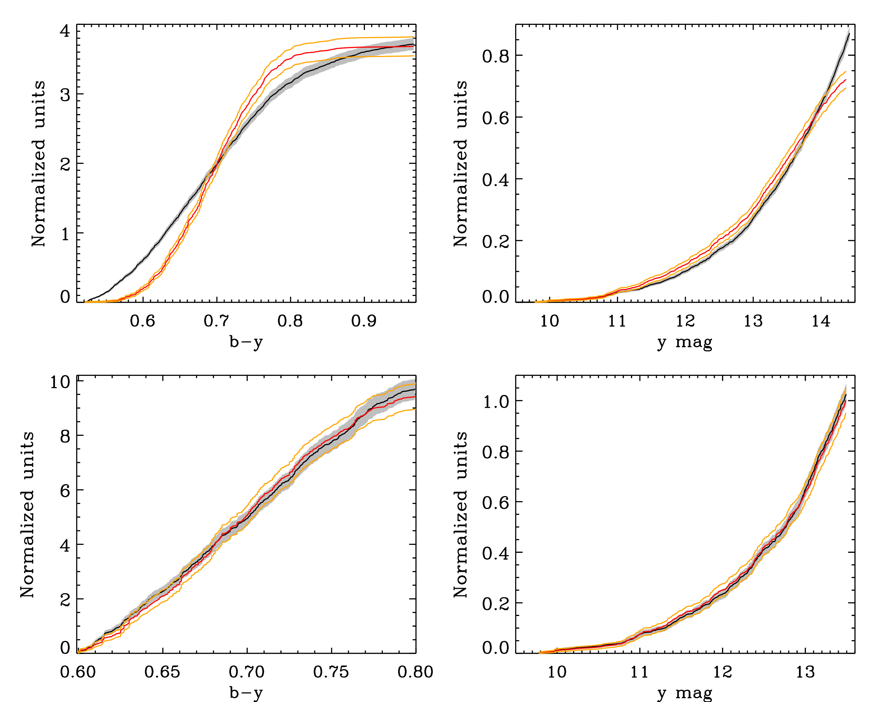
Figure 6: Top panels: cumulative distribution in $b-y$ and $y$ for the the unbiased photometric sample of giants (in black, with gray shaded area indicating $1\sigma$ Poisson errors) and the uncut asteroseismic sample of giants (in red, with orange line indicating $1\sigma$ Poisson errors) having the same colour and magnitude limits ($0.52\leq b-y\leq 0.97$ and $y\leq 14.4$). All curves are normalized to equal area. Low panels: same as above, but restricting both the asteroseismic and the unbiased photometric sample of giants to $0.6\leq b-y\leq 0.8$ and $y\leq 13.5$.

In order to have an unbiased asteroseismic sample, we must avoid the incompleteness towards the bluest and reddest colours as well as at the faintest magnitudes. We explore different cuts in $b-y$ and $y$, finding that for $0.6\leq b-y\leq 0.8$ and $y\leq 13.5$ the asteroseismic sample is representative of the underlying population of giants in the same colour and magnitude range. To this purpose, we use the Kolmogorov-Smirnov statistic on the colour and magnitude distributions: the significance levels between the asteroseismic and the unbiased photometric sample in $b-y$ and $y$ pass from $\sim 10^{-6}$ and $\sim 10^{-11}$ to about $67$ per cent and $98$ per cent respectively, when we use the cuts listed above. This implies that the null assumption that the two samples are drawn from the same population can not be rejected to a very high significance. Equally high levels of significance are obtained for the other Strömgren indices $m_{1}$ (73 per cent) and $c_{1}$ (99 per cent), as well as when the two samples are compared as function of Galactic latitude $b$ (94 per cent). For all the above parameters, significance levels of $\simeq 20$ to $80$ per cent are also obtained using different statistical indicators such as the Wilcoxon Rank-Sum test, and the F-statistic. We remark however that the unbiased photometric sample (641 targets) also includes all the seismic targets (408) within the same magnitude and colour limits. To relax this condition, we bootstrap resample the datasets $10,000$ times and find that significance levels for all of the above tests vary between $30-60$ per cent when bootstrapping either of the two samples, to $20-40$ per cent when bootstrapping both. Since for all these tests significance levels below 5 per cent are generally used to discriminate whether two samples originate from different populations, we thus conclude that the asteroseismic sample is representative of the underlying population of giants to a very high confidence level.

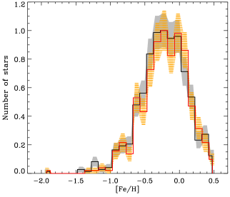
Figure 7: Normalized metallicity distribution for the unbiased photometric sample of giants (black line, with shaded gray area indicating $1\sigma$ Poisson errors) and the asteroseismic sample (red line, with shaded orange area indicating $1\sigma$ Poisson errors) in the same magnitude and colour range $0.6\leq b-y\leq 0.8$ and $y\leq 13.5$. Only stars with good photometric and metallicity flags are used.

Our photometry is significantly affected by binarity only in the case of near equal luminosity companions (or equal mass, dealing with giants at the same evolutionary stage). These binaries imprint an easily recognizable signature in the seismic frequency spectrum and are very rare (5 such cases in the full SAGA asteroseismic catalog, see discussion in Paper I). When restricting to the unbiased asteroseismic catalog three such cases survive, implying an occurrence of near equal-mass binaries of $0.7\pm 0.4$ per cent. We exclude these binaries from the analysis. Although we cannot exclude such binaries from the photometric sample, we expect the same fraction as in the asteroseismic catalog. All of the above statistical tests remain unchanged whether the asteroseismic sample with (411) or without binaries (408 targets) is benchmarked against the unbiased photometric catalog of giants, suggesting that indeed they have a negligible effect on our results.

From the above comparisons, we have already concluded that the asteroseismic sample of giants is representative of the underlying populations of giants in both colour and magnitude distribution. We expect this to be true for all other properties we are interested in as well. Whilst this is impossible to verify for masses and ages, Strömgren photometry offers a convenient way of checking this in metallicity space.

Before deriving photometric metallicities we must correct for reddening also the unbiased photometric sample (in fact, metallicities for the asteroseismic sample were derived after correcting for reddening). Interstellar extinction is rather low and well constrained in the magnitude range of our targets; we fit the $E(B-V)$ values of the asteroseismic sample as an exponential function of Galactic latitude; this functional form reflects the exponential disc used to model the spatial distribution of dust in the reddening map adopted for the asteroseismic sample (see Paper I for a discussion). The fit has a scatter $\sigma=0.015$ mag, which is well within the uncertainties at which we are able to estimate reddening. More importantly, despite this fit is based upon the asteroseismic sample (the one we want to estimate biases upon), it also reproduces (within the above scatter) the values of $E(B-V)$ obtained from 2MASS, using an independent sample of several thousand stars (see details in Paper I). Such a fit obviously misses any three-dimensional information on the distribution of dust, but the purpose here is to derive a good description of reddening for the population as a whole, in the range of magnitudes, colours, and Galactic coordinates covered in the present study.

After correcting for reddening, we apply the same giant metallicity calibration used for the asteroseismic sample (Paper I) to the photometric unbiased sample of giants, and compare the two (Figure 7). In both cases we only use stars with good photometric and metallicity flags (i.e. when the calibration is applied within its range of validity). We run the same statistical tests discussed above also for the distributions in metallicity, and significance levels varies between $15$ and $50$ per cent depending on the test and/or whether bootstrap resampling is implemented or not. Based on the above tests, we can thus conclude that for $y\leq 13.5$ and $0.6\leq b-y\leq 0.8$ the $\rm{[Fe/H]}$ distribution of the asteroseismic sample represents that of the giants in the field within the same colour and magnitude ranges.

Although we have already constrained the Kepler selection function using our Strömgren photometry, we also explore whether 2MASS photometry offers an alternative approach of assessing it, for the sake of other dataset where Strömgren is not available (e.g., such as APOKASC, Pinsonneault et al., 2014). In Figure 8a), dark-gray dots show the $K_{S}$ vs. $J-K_{S}$ colour-magnitude diagram for stars approximately in the same stripe of the asteroseismic sample ($73.4^{\circ}\leq l\leq 74.4^{\circ}$ and $7.6^{\circ}\leq b\leq 19.8^{\circ}$). In this plot, three main features are obvious: the overdensity of stars around $J-K_{S}\simeq 0.35$, which corresponds to main-sequence and turn-off stars; the overdensity at $J-K_{S}\simeq 0.65$ comprising primarily giants, and the blob at $J-K_{S}\simeq 0.85$ and faint magnitudes ($K_{S}\gtrsim 13$), mostly comprising cool dwarfs. Again, at bright magnitudes most late-type stars are giants. Overplotted with circles is the entire asteroseismic sample, including both dwarfs and giants independently of their Mflg and Pflg flags. The $K_{S}$ magnitude limit of Kepler is clearly a function of spectral type, or $J-K_{S}$ colour. Using seismic giants only, we derive the following relation between Strömgren and 2MASS magnitudes: $K_{S}=0.99\,y-3.28(J-K_{S})-0.35$, with a scatter $\sigma_{K_{S}}=0.09$ mag. The inclined black-dashed line in Figure 8a) corresponds to a constant $y=14.4$, which, as we previously saw, is roughly the limit of the faintest stars selected to measure oscillations in Kepler. At bright magnitudes, we introduce a similar cut, corresponding to $y=9.5$ (upper red-dashed line) which is approximately the saturation limit of the INT. This bright cut removes only a handful of stars and it is of limited importance. If we now compare the asteroseismic sample of giants (i.e. all giants stars with good Mflg and Pflg flags) with the entire 2MASS sample within the same magnitude limit ($9.5\leq\frac{K_{S}+0.35+3.28(J-K_{S})}{0.99}\leq 14.4$) and colour range ($0.494\leq J-K_{S}\leq 0.951$), the hypothesis that two samples are drawn from the same population is rejected. The same is still the case if we use a constant magnitude cut $6\leq K_{S}\leq 12$ (such to encompass our sample, see Fig. 8a) instead of the colour dependent one done above.

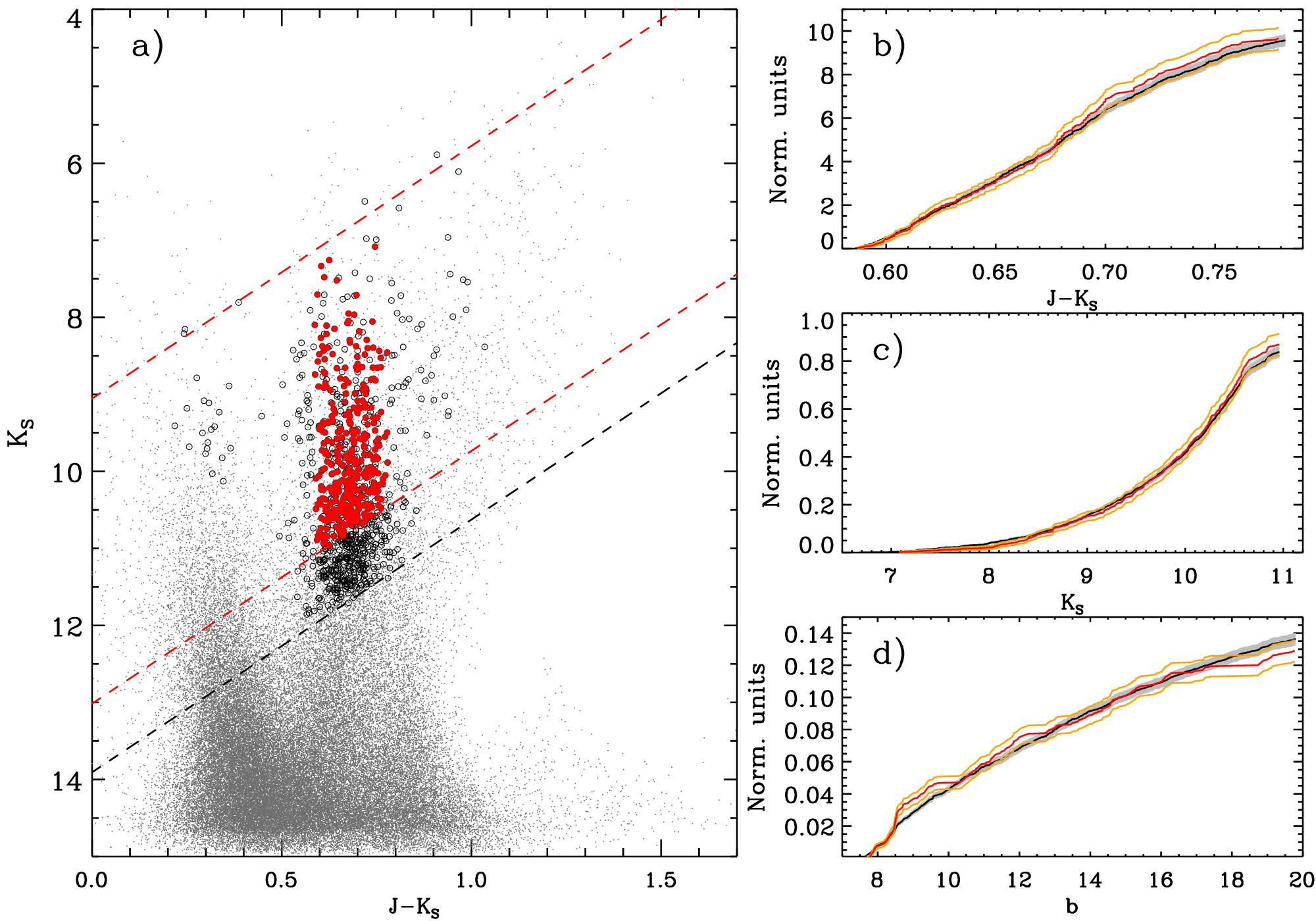
Figure 8: Left panel: 2MASS $K_{S}$ vs. $J-K_{S}$ diagram (gray dots) for stars in approximately the same Galactic stripe of the asteroseismic sample (black open circles). Filled red circles identify stars belonging to the unbiased asteroseismic sample built as described in the text, i.e. having good photometric and metallicity flags, and with $0.586\leq J-K_{S}\leq 0.782$ and $K_{S}\leq 13.01-3.28\,(J-K_{S})$. Right panels: cumulative distributions between the unbiased 2MASS photometic sample and seismic giants with same colour and magnitude cuts (colour code same as of Figure 6).

From the Strömgren analysis we already know the magnitude and colour range where the asteroseismic targets are expected, on average, to unbiasedly sample the underlying population of giants. Thus, we can see how these limits convert in the 2MASS system. Using all seismic targets we derive the following relation $J-K_{S}=0.977\,(b-y)$ with $\sigma_{J-K_{S}}=0.04$, which converts $0.6\leq b-y\leq 0.8$ into $0.586\leq J-K_{S}\leq 0.782$. We also apply a colour dependent $K_{S}$ magnitude cut corresponding to $9.5\leq y\leq 13.5$ (filled red circles and red-dashed lines in Figure 8a). In this case, the seismic and 2MASS samples are drawn from the same population to statistically significant levels in colour, magnitude and Galactic latitude distribution, as qualitatively shown on the right-hand side panels of Figure 8.

4 Vertical Mass and Age Gradients in the Milky Way disc

The Kepler field encompasses stars located in the direction of the Orion arm, edging toward the Perseus, and rising above the Galactic plane. The stripe observed so far by SAGA has Galactic longitude $l\simeq 74^{\circ}$ and covers latitude $8^{\circ}\lesssim b\lesssim 20^{\circ}$. Its location in the Galactic context is shown in Figure 9; it can be immediately appreciated from panel a) and b) that the geometry of the SAGA survey allows us to probe distances of several kpc from the Sun at nearly the same Galactocentric radius, thus minimizing radial variations and greatly simplifying studies of the vertical structure of the Milky Way disc. At the same time, SAGA spans a vertical distance Z (altitude or height, hereafter) of about $1.5$ kpc, probing the transition between the thin and the thick disc, which have scale-heights of $\simeq 0.3$ and $\simeq 1$ kpc, respectively (e.g., Jurić et al., 2008). In Figure 10 we show the raw dependence of stellar ages and masses with Galactic height, as well as the raw age-metallicity relation. For the purpose of Galactic studies, these plots can not be taken at face value, and must first be corrected for target selection effects (stemming from the colour and magnitude cuts derived in the previous Section), as well as to account for the fact that in the most general case, the ages of red giants might not be representative of those of an underlying stellar population. These steps are described further below.

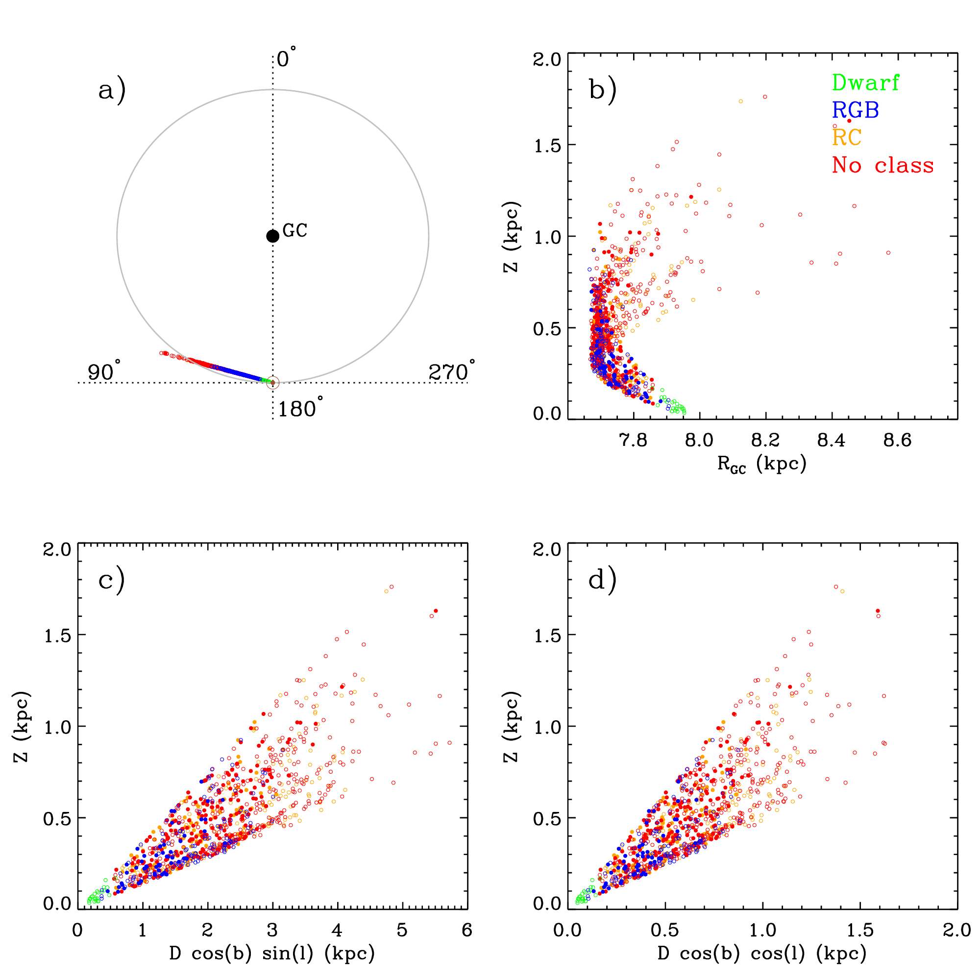
Figure 9: Location of the SAGA targets in Galactic coordinates. Stars with different colours have different seismic evolutionary classification “Dwarf”, “RGB”, “RC” and “NO” as indicated. Filled circles identify the 373 stars which satisfy the constraints described in Section 4. Panel a): target distribution over the Galactic plane, where the distance of each seismic target from the Sun ($D$) is projected along the line of sight $D\,\cos(b)$ having direction $l\simeq 74^{\circ}$ and Galactic latitude $b$. The distance between the Galactic Centre (GC) and the location of the Sun ($\odot$) is marked by the gray circle. Galactic longitudes ($l$) at four different angles are indicated. Panel b): same as above, but as function of Galactic height $\textrm{Z}=D\,\sin(b)$ and Galactocentric Radius ($\rm{R_{GC}}$, computed assuming a solar distance of $8$ kpc from the Galactic Centre). Panel c) and d): Z distribution of targets across two orthogonal directions. The multiple beams structure in panels b) to d) arises from the projection of the gaps in the CCD modules on Kepler.

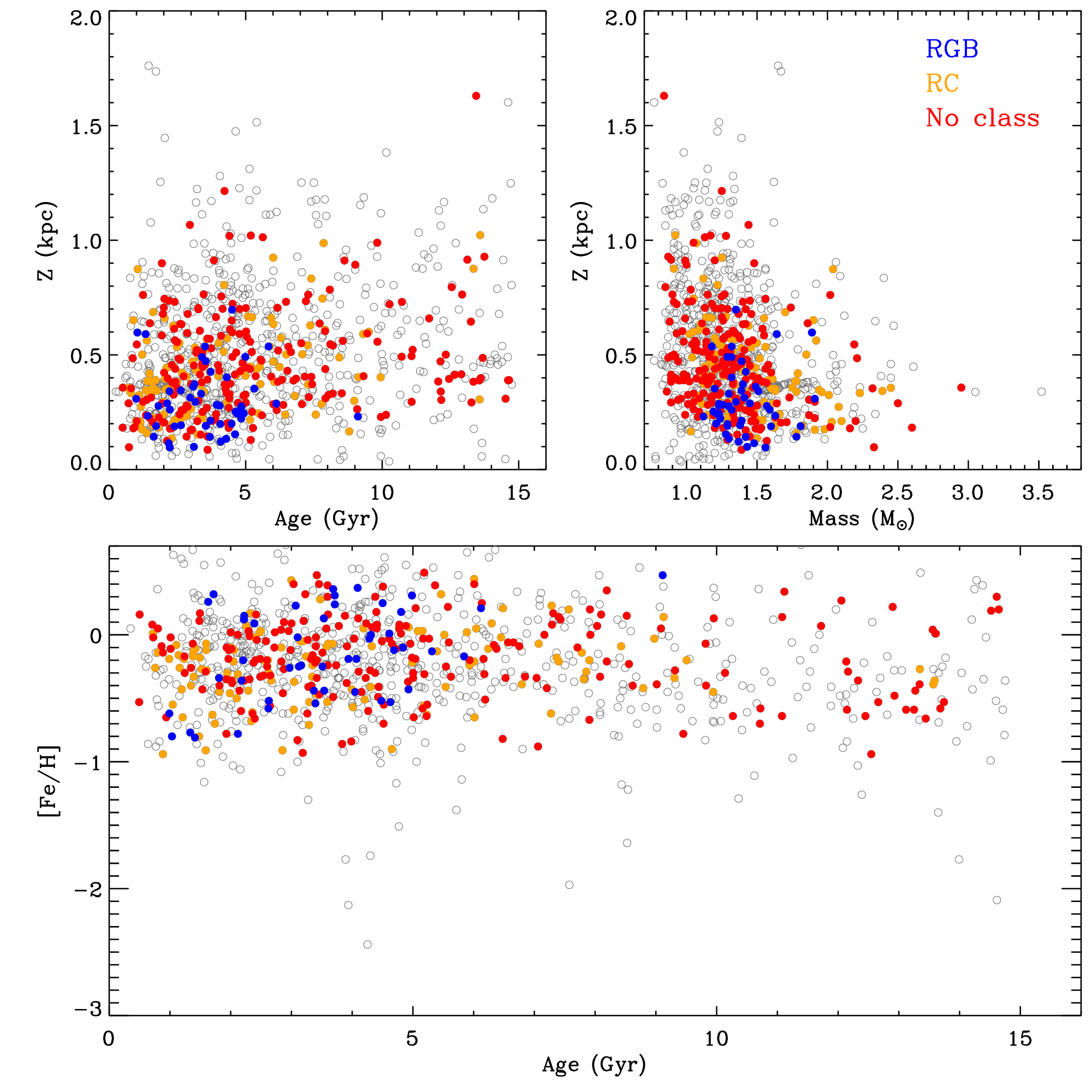
Figure 10: Raw age and mass gradients (top panels) and age-metallicity relation (lower panel) before correcting for completness and target selection. Open circles are all giants in SAGA, while filled circles (colour coded according to their seismic classification) are stars satisfying the seismic target selection discussed in Section 4.1.

4.1 Sample selection

To estimate gradients, we limit our sample to $0.6\leq b-y\leq 0.8$ and $y\leq 13.5$ such that it reflects the distribution of the underlying sample of giants (Section 3). We remove stars labelled as binaries and those flagged as having poor photometry and/or metallicity estimates (see Section 2). The latter requirement automatically excludes stars with $\rm{[Fe/H]}\geqslant 0.5$, but we also limit the metallicity range to $\rm{[Fe/H]}>-1.0$, to remove any halo object, which would contaminate our study of disc gradients. By excluding metal-poor stars we also avoid problems related to the potential inaccuracy of seismic scaling relations in this regime (Epstein et al., 2014). Because we are interested in studying properties of the Galactic disc via field stars, we also exclude members of the open cluster NGC 6819, based on their seismic membership. Furthermore, we remove all targets classified as “Dwarf”, obtaining a final sample of 373 giants (i.e. with seismic evolutionary classification “RGB”, “RC” or “NO”, see Section 2.2). They cover heights from $\approx 0.1$ to $1.5$ kpc (Figures 9 and 10). From the above sample of giants, we also extract a subsample of 48 seismically classified “RGB” stars with age uncertainties less than 30 per cent. As discussed in Section 2.3, mass-loss can severely affect age estimates of unclassified and clump stars, whereas “RGB” stars are essentially immune to such uncertainty. These stars provide more robust ages, though at the price of a greatly reduced sample size. We also refer to Paper I for the uncertainties associated to masses and distances, which are of order 6 and 4 per cent, respectively. In the following we will determine vertical gradients using both samples whenever possible: the 373 “Giants” and the 48 best pedigreed “RGB” stars. The bulk of gravities for the “Giants” sample covers the range $2.0<\log g<3.5$, while for “RGB” stars covers $2.6<\log g<3.35$: we will use these values when modelling target selection in Section 4.3.

4.2 Methodology and raw vertical gradients

We adopt two methodologies to estimate the vertical gradient of age and mass. First i) we use a boxcar-smoothing technique described in Schlesinger et al. (2015). Sorting the stars by height above the plane, we calculate the median age (mass) and altitude Z of a fraction of the sample at the lowest height. We then step through the sample in altitude, as we want to quantify the age (mass) variation with height above the plane. Each bin contains the same number of stars and overlaps by a small fraction with the previous bin. For the “Giants” sample, we explore the range between 18 and 30 stars per bin with overlaps ranging from 8 to 15. The “RGB” sample is much smaller and we explore the range between 8 and 10 stars per bin with overlaps ranging from 2 to 4 stars. The binsizes and overlaps explored contain enough targets so that the overall trend is not dominated by outliers, and the median points well reflect the overall behaviour of the underlying sample. We then perform a least-squares fit on these median points; the change in slope (i.e. gradient) due to different choices of binsize and overlap is typically below half the uncertainty of the fit parameter itself. We perform a Monte-Carlo to explore the sensitivity of the boxcar-smoothing on the uncertainty of the input ages (masses), and add this uncertainty in quadrature to those estimated above. We obtain the following raw age and mass gradients for the “Giants” $3.9\pm 1.1$ Gyr kpc^-1, $-0.39\pm 0.10\,\rm{M}_{\odot}$ kpc^-1. Similarly, for the “RGB” stars we have $-0.1\pm 3.3$ Gyr kpc^-1, $-0.09\pm 0.35\,\rm{M}_{\odot}$ kpc^-1.

Our second estimate of the gradient ii) consists of a simple least-squares fit to all of the stars that meet our criteria. Again our uncertainties include those from the fitting coefficients and from a Monte-Carlo. In this case we obtain for the “Giants” $4.1\pm 0.9$ Gyr kpc^-1, $-0.43\pm 0.08\,\rm{M}_{\odot}$ kpc^-1 and for the “RGB” stars $0\pm 1.7$ Gyr kpc^-1, $0.03\pm 0.20\,\rm{M}_{\odot}$ kpc^-1.

With both methods, the gradients for the “RGB” stars have considerably larger uncertainties, which make them consistent with no slope and limit their usability to derive meaningful conclusions. This is due to the small sample size and scatter of the points. Because of this, the $\chi^{2}$ of the “RGB” fits have the same statistical significance whether we let the slope and intercept be free, or we fix the latter on the “Giants” sample (roughly 3 Gyr and $1.5\,\rm{M}_{\odot}$ on the plane). With this caveat in mind (i.e. fixing the intercept), and including in the error budget the uncertainty in the intercept derived from the “Giants”, the raw “RGB” slopes become $3.6\pm 1.7$ Gyr kpc^-1 and $-0.43\pm 0.17\,\rm{M}_{\odot}$ kpc^-1 for method i), and $1.4\pm 1.2$ Gyr kpc^-1 and $-0.39\pm 0.14\,\rm{M}_{\odot}$ kpc^-1 for method ii).

Technique i) and ii) have different strengths; as the sample size is small, the least-squares fit takes full advantage of every star available. However, the boxcar-smoothing technique avoids being skewed by any outliers. Additionally, we can see how the uncertainties vary with respect to height above the plane by examining the variation in each median point.

We stress that both methods still need to be corrected for target selection effects, i.e. the gradients above should not be quoted as the values obtained for the Galactic disc. Also, the use of stellar masses as proxy for stellar ages is applicable only to red giants. Thus, while it is meaningful to derive a Galactic age gradient by assessing how well our sample of red giants (with known selection function) will convey the age structure of the larger underlying stellar population (done in the next Section), the stellar mass gradient will reflect the mass structure of the underlying population of red-giants only. For red giants, the relation between mass and age is $\textrm{Age}\propto M^{-\alpha}$, with $\alpha\simeq 2.5$. Thus, we expect that the age gradient traced by red giants translates into a variety of masses at the youngest ages, whereas low-mass (i.e. old) stars will be preferentially found at higher altitudes. Indeed, this picture is consistent with Figure 10, which shows an L-shaped distribution of red-giants, with low-mass stars extending from low to large heights and more massive stars being preferentially close to the Galactic plane. Because of the aforementioned power-law relationship between age and mass, one might wonder whether a linear fit is appropriate for quantifying the mass gradient shown by red giants. In fact, a change of say $0.2\rm{M}_{\odot}$ translates to a few 100 Myr in a $2\rm{M}_{\odot}$ star, but corresponds to several Gyr at solar mass. Here, our goal is not to provide a value for the mass gradient –which given the above discussion would be of limited utility– but simply to use the masses of our red giants as a model independent signature of the vertical age gradient. The above fits of the mass gradient suffice for this purpose, and in the following discussion we will focus only on the vertical age gradient.

4.3 Correcting for target selection

In Section 3 we have studied the Kepler selection function to determine the colour and magnitude ranges in which the SAGA asteroseismic sample reflects the properties of an underlying unbiased photometric sample of red giants. However, to derive the Galactic age gradient we must assess how target selection systematically affects our gradient estimates (i.e. once a clear selection function is defined, we must assess its effect). To avoid our results being too depend on particular model assumptions, we use various approaches to understand how our selection criteria and survey geometry will bias our sample, and to what extent the ages of a population of red giants are representative of the ages of a full stellar population.

Figure 11: Probability of a star passing the “Giants” target selection to be observed given its height, metallicity and age (see description in Section 4.3.1). All probabilities are normalized to an arbitrary scale.

4.3.1 Target selection modelling

We first want to examine the probability that a star with specific stellar parameters will be observed given our target selection criteria. We generate a data-cube in age, metallicity and distance where each point in the age and metallicity plane is populated according to a Salpeter IMF over the BaSTI isochrones. For each of these populations we then assign apparent magnitudes by running over the distance dimension in the cube. Thus, for each combination of age, metallicity and distance we can define the probability of a star being observed by SAGA as the ratio between how many stars populate that given point in the cube, and how many pass our sample selection (i.e. our color, magnitude and gravity cuts, see Section 4.1). This approach naturally accounts for the effects of age and metallicity on the location of a star on the HR diagram. Via the IMF it also accounts for the fact that stars of different masses have different evolutionary timescales, and thus different likelihood of being age tracers of a given population. This approach is the least model dependent, and provides an elegant way to gauge the selection function.

Figure 11 shows the probability of each star being observed given its height, metallicity and age. Our sample is biased against stars at large distances (and thus altitudes), low metallicities, and old ages.

We can then apply methodology i) and ii) described in Section 4.2, where in the boxcar-smoothing/fitting procedure we assign to each star a weight proportional to the inverse of its probability. Stars with low probability will be given larger weight to compensate for the fact that target selection is biased against them. Figure 11 indicates that probabilities are non linear functions of the input parameters; for some targets the combination of age, metallicity and distance results in a probability of zero, which then translates into an unphysical weight. Observational errors are mainly responsible for scattering stars into regions not allowed in the probability space. To cope with this effect without setting an arbitrary threshold on the probability level, for each target we compute the probability obtained by sampling the range of values allowed by its age, metallicity and distance uncertainties with a Monte-Carlo. While this procedure barely changes the probabilities of targets very likely to be observed, it removes all null values. Depending on the method and sample (Section 4.2), factoring these probabilities in the linear fit typically increases the raw age gradient (Table 1).

4.3.2 Population synthesis modelling

Our second method to explore target selection effects also relies on population synthesis. However, rather than generating a probability data-cube, we produce a synthetic population with a certain star formation history, metallicity distribution function, IMF, and stellar density profile. This gives us the flexibility of varying each of the input parameters at the time, to explore their impact on a population.

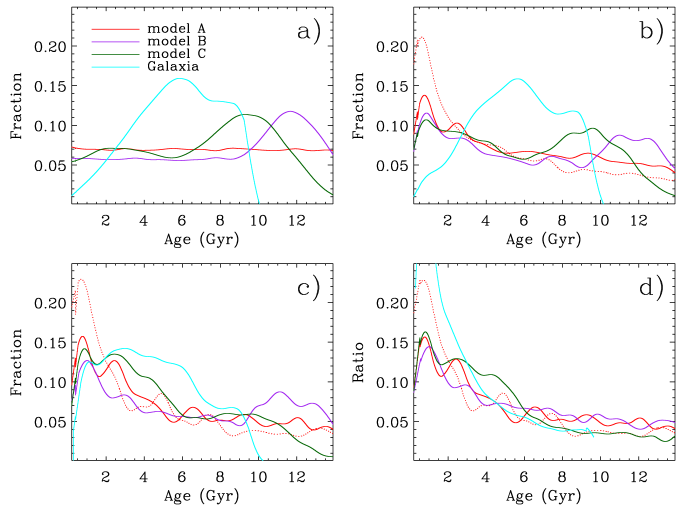
Figure 12: Panel a): age distribution input in different models, as traced by low-mass, unevolved stars. Panel b): the same distributions when restricting to stars with $2.0<\log g<3.5$. Dotted red line is when changing the IMF in model A to have $\alpha=-1.35$. Panel c): age distributions when applying the SAGA “Giants” target selection: $2.0<\log g<3.5$, $10\leq y\leq 13.5$, $0.6\leq b-y\leq 0.8$ and $\rm{[Fe/H]}>-1$. Panel d): ratio between the outputs in panel c) and the inputs in panel a). All curves are normalized to equal area. Small wiggles are due to realization noise.

We assume a vertical stellar density profile described by two exponential functions with scale-heights of $0.3$ and $1.2$ kpc, to mimic the thin and the thick disc, respectively. For our tests, we define three models; in our first one (A) we adopt a constant star formation history over cosmic time, meaning that each age has a probability of occurring $1/\tau_{max}$, where $\tau_{max}$ is the maximum age covered by the isochrones. We also assume a flat metallicity distribution function over the entire range of the BaSTI isochrones and a Salpeter IMF. Shallower and a steeper slopes for the IMF are also explored ($\alpha\pm 1$).

Our second model (B) is very similar to the previous one, the only difference being a burst of star formation centred at 12 Gyr (50 per cent of the stars), followed by a flat age distribution until the present day. Note that in both model A and B ages are assigned independently of their thin or thick disc membership, and no vertical age gradient is present.

In our last model (C) we describe the ages of thin disc stars with a standard gamma distribution (with $\gamma=2$) having a dispersion of $2.5$ Gyr, centred at zero on the Galactic plane, and with a vertical gradient of $4.5$ Gyr kpc^-1. For thick disc stars we adopt a Gaussian distribution centred at 10 Gyr with a dispersion of $2$ Gyr. The metallicity distribution function of thin disc stars is modelled by a Gaussian centred at solar metallicity on the plane, with a dispersion of $0.2$ dex and a vertical gradient of $-0.2$ dex kpc^-1. For the thick disc we assume a Gaussian metallicity distribution centred at $\rm{[Fe/H]}=-0.5$ with dispersion of $0.25$ dex. While model C provides a phenomenological description of some of the features we observe in the Milky Way disc, it is far from being a complete representation of it, which is not our goal anyway. A more complete Milky Way model is explored in the next Section using Galaxia (Sharma et al., 2011).

Here, we simply want to explore selection effects, in particular on stellar ages. Figure 12 shows how the age distribution input in different models (traced by unevolved low mass stars, panel a) is altered when selecting evolved stars (defined as having $2.0<\log g<3.5$, panel b) or applying the SAGA “Giants” target selection discussed in Section 4.1 (panel c). It is clear that even in the simplest case (model A), the age distribution of “Giants” is strongly biased towards young stars (panel d), in agreement to what we already deduced from Figure 11. This is driven by the combined effect of evolutionary timescales and the slope of the IMF (compare continuous and dotted line for model A).

We first compute the gradient input in each model using its unevolved stars, defined here as all stars with masses below $0.7M_{\odot}$. Because of the large dispersion of ages at each height (also present in Galaxia, see next Section), we find that fitting heights as function of ages –i.e. to derive a slope in kpc Gyr^-1– provides a better description of the data. From the population synthesis volume, we extract a pencil beam with Galactic latitudes $8^{\circ}<b<20^{\circ}$, apply the target selection of “Giants” and “RGB” stars and compute the kpc Gyr^-1 slopes of these sub-samples. The change in slope between the unevolved-stars and the target-selected ones defines the correction that must be applied to the raw data. Thus, we use the correction in slope determined above to modify the observed SAGA values, by adjusting the height of each star depending on its age. This adjustment increasingly affects older stars, which are lifted in altitude Z after correcting for target selection. In reality, the position of each of our targets is well determined (within its observational uncertainties): the change we introduce here is simply meant to counteract the bias introduced into the distribution by target selection. This is to say that if our sample were not affected by target selection, we would preferentially observe additional stars at higher Z. Once we adjust the height of each of our objects as described, we then perform a least-squares fit on the shifted points in terms of Gyr kpc^-1. We apply a similar technique to our boxcar-smoothing analysis except here, rather than shifting every star, we shift each median point and re-fit them with a least-squares in Gyr kpc^-1. Thus, although we apply the same target selection correction, its effect will be different. Because there is a much wider range of values star-by-star than in the median points, the gradient from the least-squares analysis changes more than for the boxcar-smoothing. Also in this case, correcting for target selection typically increase the raw SAGA gradients by a few Gyr kpc^-1 (Table 1).

4.3.3 Galaxy modelling

By applying our target selection criteria to a model of the Galaxy, we can determine how well the resulting sample reflects the disc behaviour assumed by the model. For this purpose we simulate the SAGA stripe using Galaxia (Sharma et al., 2011).

Galaxia is based on the Besancon analytical model of the Milky Way (Robin et al., 2003); the disc is composed of six different populations with a range of ages from 0 to 10 Gyr. The thick disc and halo are modelled as single-burst, metal-poor populations of 11 and 14 Gyr, respectively. For our analysis, we limit ourselves to the six thin-disc populations in Galaxia; this age range is representative of the bulk of the SAGA sample with a more continuous distribution in age and chemistry than if we used also the single-burst populations. Although the origin of the thick disc is still unclear, it is unlikely to consist of stars having a single age and it might also span a large metallicity range (see discussion in the Introduction). Galaxia itself is a sophisticated –yet simplified– representation of the Galaxy, which assumes a certain age and metallicity distribution for each Galactic component. Among other things the metallicity scale, the stellar radii, gravities, synthetic colours, model $T_{\rm{eff}}$ along the red giant branch and mass-loss prescription will also depend on the isochrones implemented in the model, which are from Padova in the case of Galaxia (Bertelli et al., 1994; Marigo et al., 2008). We do not attempt to vary any of the Galaxia ingredients, and we have already explored the effect of changing some of those assumptions using the population synthesis approach described in the previous Section.

Here, we want to further assess how a known input population from a realistic Galactic model will appear once filtered through our target selection algorithm. We adopt the same technique described in Section 4.3.2. We calculate the input gradient using unevolved stars, implement the “Giants” and “RGB” target selection on the Galaxia simulated stars to derive corrections in kpc Gyr^-1, and apply those to the data before re-fitting the gradient in Gyr kpc^-1. The age distribution input in Galaxia is rather different from that traced by our simplistic population synthesis models, and it does not extend beyond 10 Gyr because of the thick disc exclusion (Figure 12).

The Galaxia model shows a wide range of ages at each height above the Galactic plane; however, the proportion of young stars diminishes as the height increases, resulting in typically older ages far away from the Galactic plane. The SAGA cuts in colour and magnitude remove many of the older stars at large heights: this boosts the fraction of young stars and skews the sample to lower heights in accordance to what we already derived in Section 4.3.1 and 4.3.2. Target selection corrections are similar to what we derived previously, and of the order of few Gyr kpc^-1.

4.3.4 Correlation with distances

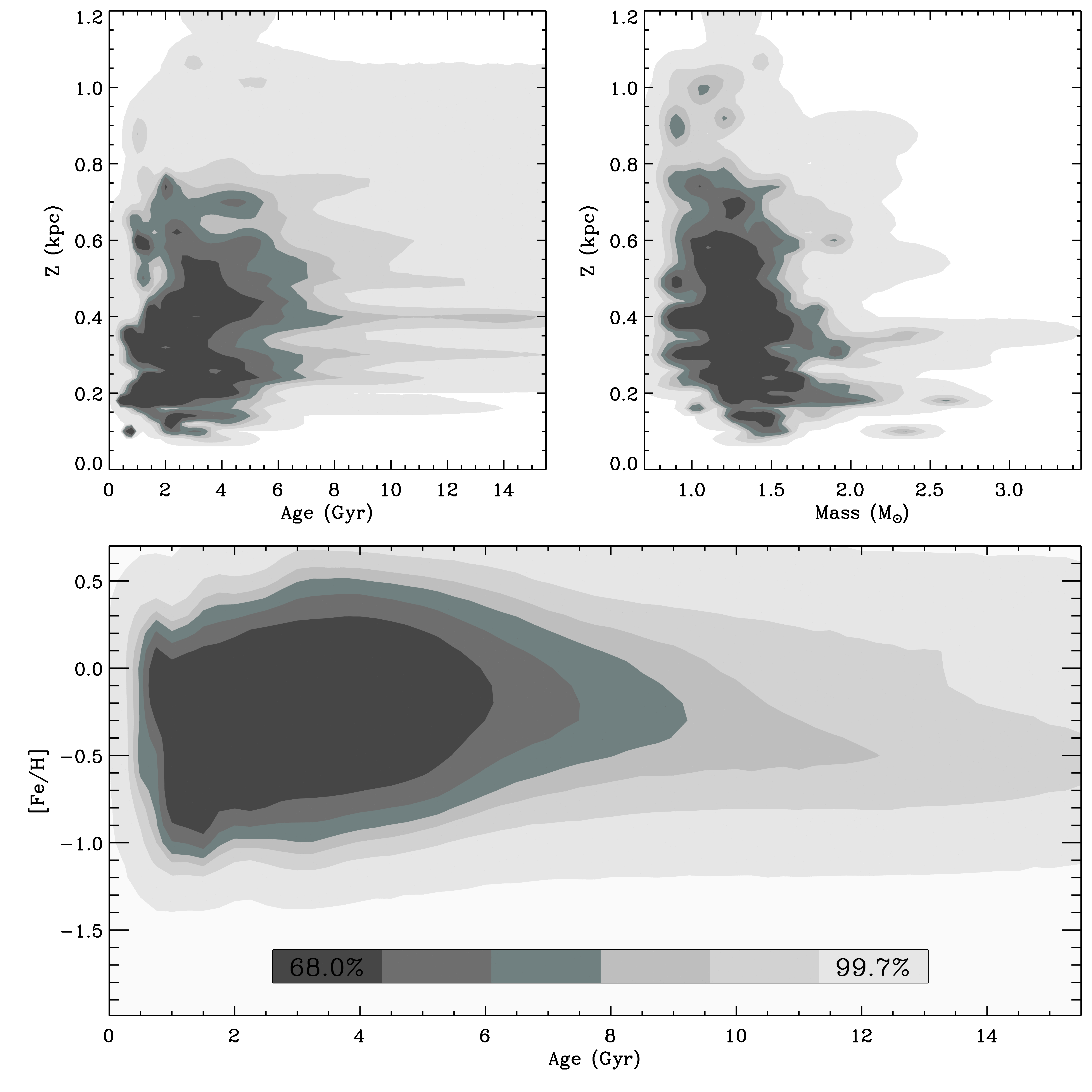
Figure 13: Age and mass gradients (top panels) and age-metallicity relation (lower panel) after correcting for target selection the “Giants” sample. Contour levels have been obtained by convolving each star with its age, distance and metallicity uncertainties and assigning a density proportional to the logarithm of the inverse probability of being observed. Probabilities have been computed as described in Section 4.3.1.

In a pencil-beam sample such as SAGA, the average altitude $\textrm{Z}=D\sin(b)$ will, by the geometry, rise almost linearly with distance $D$; hence the two quantities are strongly correlated. Thus, any correlation for example of age with distance, will bias the gradient derived as function of Z. This effect can be accounted for by introducing the dependence on distance in the least-squares fit when deriving the gradients (e.g. Schönrich et al., 2014). This technique provides a model-independent check (modulo the degree at which giants trace the ages of an underlying stellar population). Assuming that a (multi) linear dependence provides a reasonable description of the underlying structure of the data (which over the range of distances studied here is appropriate for ages), one can expand the fit into

$$\tau_{i}=\frac{d\tau}{d\textrm{Z}}\textrm{Z}_{i}+\frac{d\tau}{dD}D_{i}+\epsilon$$ (2)

where $i$ is the index running over the stellar sample, $d\tau/d\rm{Z}$ and $d\tau/dD$ are the free fit parameters measuring the correlation between age $\tau$, altitude Z and distance $D$, and $\epsilon$ is the intercept of the fit. When we apply this technique to SAGA, the significance of the derived slopes is usually above three sigma for the “Giants” sample, whereas it is below 1 sigma for “RGB” stars due to the smaller sample size and range of distances. Thus, we apply this method only to “Giants”.

Accounting for the distance dependence returns a least-squares gradient of $6.3\pm 1.6$ Gyr kpc^-1. The increase with respect to the value of $4.1\pm 0.9$ Gyr kpc^-1 obtained with a simple linear fit (Section 4.2) tells us that the survey geometry is indeed biased against old stars, and thus any fit of the raw data underestimate the true age gradient.

4.4 The vertical age gradient

In Section 4.2 we have used two different methods and samples to measure the raw vertical age gradient with SAGA. We have then assessed target selection effects using different approaches. Although they return a range of values for the correction, they all consistently show that any raw measurement of the vertical age gradient using red giants underestimates the real underlying value.

We summarize the raw gradients obtained using different samples and methods in Table 1, along with the target selection corrections discussed in Section 4.3.1 to 4.3.3. For each method and sample listed in the table, we compute the median target selection correction and standard deviation as a measure of its uncertainty. This is added in quadrature to the undertainty derived for each fit, after which the weighted average of all gradients is computed, obtainining a value of $4.3\pm 1.6$ Gyr kpc^-1. If we instead replace the “RGB” slopes with those obtained without forcing the intercept, then we obtain a weighted average of $3.9\pm 2.5$ Gyr kpc^-1. Hence, the gradient does not change dramatically, but its uncertainty is increased.

Table 1: Target selection effects. Corrections are intended to be summed to the raw vertical gradients. All values are in Gyr kpc^-1.

		Corrections from	Corrections from			Corrections from
	Raw gradients	target selection	population synthesis			Galactic
		modelling	modelling			modelling
			A	B	C
boxcar	$+3.9\pm 1.1$	$+0.6$	$+0.2$	$+0.3$	$+0.1$	$+0.0$	“Giants”
smoothing	$+3.6\pm 1.7$	$+1.2$	$+1.4$	$+1.2$	$+3.5$	$+3.4$	“RGB”
least-squares	$+4.1\pm 0.9$	$+3.7$	$+2.4$	$+1.2$	$+2.7$	$+3.8$	“Giants”
fit	$+1.4\pm 1.2$	$-1.0$	$+1.8$	$+1.3$	$+5.3$	$+4.8$	“RGB”

The raw gradients quoted for the “RGB” sample are obtained forcing the intercept of the fit. If kept unconstrained, the raw “RGB” values would change to $-0.1\pm 3.3$ and $0\pm 1.7$ Gyr kpc^-1.

While all the above values clearly indicate that the age of the Galactic disc increases when moving away from the plane, the consistency among different samples, methods and target selection corrections vary. It should also be kept in mind that mass-loss changes our age estimates. If we were to adopt the ages derived for SAGA assuming an efficient mass-loss ($\eta=0.4$), the raw gradients for the “Giants” sample would decrease by $1.3$ Gyr kpc^-1. Since the effect of mass-loss for the SAGA “RGB” stars is negligible, their gradient decreases by only $0.2$ Gyr kpc^-1.

Based on the above discussion, we conclude that in the region of the Galactic disc probed by our sample, the vertical age gradient is on the order of $4.0\pm 2.$ Gyr kpc^-1, which also encompasses the uncertainty stemming from mass-loss. In particular, it should be stressed that at any given height there is a wide range of ages. Figure 13 shows such overdensities in the vertical age, mass and age-metallicity relation when including observational uncertainties and correcting for target selection.

To our knowledge, the present study is the first of this kind, quantifying the in situ vertical age gradient of the Milky Way disc. While the origin of this age gradient is beyond the scope of this paper, its existence has long been known by indirect evidence such as e.g. the age-velocity dispersion relation (e.g. von Hoerner, 1960; Mayor, 1974; Wielen, 1977; Holmberg et al., 2007), the chemistry in red giants (Masseron & Gilmore, 2015) and the change in fraction of active M dwarfs of similar spectral type at increasing Galactic latitudes (e.g., West et al., 2011, and references therein). However none of these studies is able to provide a direct measurement as we do here.

5 The age-metallicity relation of disc red giants and their age distribution

An important constraint for Galactic models is provided by the time evolution of the metal enrichment, the so-called age-metallicity relation. The strength or even the existence of this relation among disc stars has been largely debated in the literature because of the intrinsic difficulty of deriving reliable ages for field stars, as well as issues with sample selection biases (e.g., McClure & Tinsley, 1976; Twarog, 1980; Edvardsson et al., 1993; Ng & Bertelli, 1998; Rocha-Pinto et al., 2000; Feltzing et al., 2001). We can now take a fresh look at this issue, with the first age-metallicity relation from seismology shown in Figure 10 for the entire dataset, as well as when restricting only to “Giants”. The SAGA target selection intrinsically favours metal-rich, young stars thus flattening the overall age-metallicity. If we adopt the age ($\simeq 4\pm 2$ Gyr kpc^-1) and metallicity gradients ($\simeq-0.2\pm 0.1$ dex kpc^-1, Schlesinger et al., 2015) measured over the SAGA stripe we obtain a shallow slope of $-0.05\pm 0.06$ dex Gyr^-1. This is consistent with what is obtained instead if we were fitting the age-metallicity in Figure 10, and correcting for target selection afterwards. Seismology thus confirm the rather mild slope and large spread at all ages in the age-metallicity relation of disc stars, as already derived from turn-off and subgiant stars in the solar neighbourhood (e.g., Nordström et al., 2004; Haywood, 2008; Casagrande et al., 2011; Bergemann et al., 2014) and also in agreement with the study of Galactic open clusters (e.g., Friel, 1995; Carraro et al., 1998, see also Leaman et al. 2013 for the age-metallicity relation of disc globular clusters). It should also be noted that a typical age uncertainty of order 20 per cent implies a much larger absolute number at older ages than at younger ones (i.e. $10\pm 2$ Gyr versus $1\pm 0.2$ Gyr). Thus, despite old and metal-rich stars do exist, when convolving their uncertainties in the age-metallicity relation their contribution is much reduced (compare Figure 10 with Figure 13). Also, our sample selection limits us to $\rm{[Fe/H]}>-1$, preventing us from tracing the early enrichment expected in the age-metallicity relation (compare e.g. the steep rise in metallicity at about 13 Gyr in figure 16 of Casagrande et al. 2011).

Figure 14 shows the age distribution for the “Giants” sample. Overall this is similar to what we have already discussed in Section 2.3, apart from the fact that we are now applying completness cuts. A significant overdensity seems to appear at the oldest ages, above $\simeq 10$ Gyr, which persist also when adopting ages computed with mass-loss. We know that our target selection is biased against old stars (Section 4.3), and it would thus be intriguing to interpret this overdensity as the signature of a population formed/accreated early in the history of the Galaxy. As we have discussed in Section 4.3.2, a constant star formation rate produces an age distribution of red giants which peaks at young values, and with a long tail. A strong burst in star formation at a given age manifests instead as a localised peak at that epoch (see Figure 12).

Figure 14: Panel a): age distribution (with Poisson error bars) for the “Giants” sample. Panel b) and c): same as above, but for $\rm{Z}\geq 0.5$ kpc and $\rm{Z}<0.5$ kpc, respectively.

We only select stars with $\rm{[Fe/H]}>-1$, implying that this overdensity is associated with disc stars, rather than the halo, and it could be the signature e.g., associated to the formation of the thick disc or enhanced star formation in the early Galaxy (c.f. Haywood et al., 2013; Robin et al., 2014; Snaith et al., 2014). Because of the vertical age gradient and the survey geometry we must first verify whether this overdensity could simply stem from stars at the highest Z. Correcting the histogram for the vertical age gradient is not straightforward since we have a mixture of young and old stars at all heights, and this would unphysically shift part of the age histogram at negative values. We therefore split the age distribution below and above $\textrm{Z}=0.5$ kpc in Figure 14b) and c). A moderate overdensity at the oldest ages is still present in both panels. However, when we fold age uncertainties in the histogram, the overdensity at old ages disappears, consistently with the lower panel in Figure 13.

We thus conclude that the detection of a peak at old ages is not significant and emphasize the importance of taking proper age uncertainties into consideration when conducting this kind of analysis. Future larger datasets with improved age precision will be able to look for the existence of signatures of this kind. With our current SAGA sample, we can rule out the presence of any major overdensity at ages younger than about 10 Gyr, implying that the Milky Way disc had a relatively quiescent evolution since a redshift of about 2 (see also Ruchti et al., 2015). Increasingly sophisticated cosmological simulations are now able to predict gross morphological properties on galactic scales (Torrey et al., 2012; Vogelsberger et al., 2014), yet the survival of discs seem to critically depend on the abscence of violent events (Scannapieco et al., 2009); our results support such scenario.

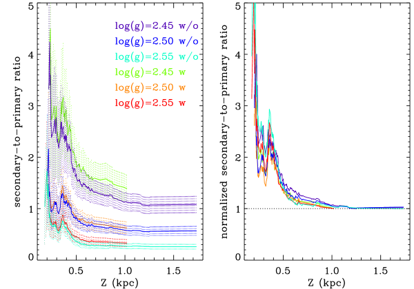
Figure 15: Left panel: ratio between the (cumulative) number of secondary to primary clump stars and function of height from the plane Z. Different colours indicate the adopted surface gravity cut to discriminate between primary and secondary clump, whether with (w) or without (w/o) completness cuts. Dotted areas indicate Poisson’s errors. Right panel: same plot but normalizing each curve to the value at the highest altitude Z.

6 Secondary clump stars: standard age candles for Galactic Archaeology

The secondary clump is populated by stars which ignite helium in (partly) nondegenerate conditions, and it is a phase relatively well-defined in time (e.g., Girardi, 1999). Although the precise mass and hence age, at which this happens depend on the models themselves, secondary clump stars define a nearly pure population of young ($\lesssim 2$ Gyr) stars. At the youngest ages the intrinsic luminosity of clump stars is non constant, thus making them unsuitable distance calibrators (Chen et al., in prep); nevertheless as we show below, secondary clump stars can be used as standard age candles to estimate i) the intrinsic metallicity spread at young ages, and ii) to trace the aging of the Galactic disc.

i) We have already shown that thanks to our precise seismic $\log g$ determinations we can discriminate between primary and secondary clump stars in a field population (see also Paper I, figure 17). Here, we use only stars with secure “RC” classification and adopt a fixed $\log g=2.5$ to discriminate between the two phases. This cut is rather arbitrary, although we have verified that our results still hold for reasonable variations of this threshold. After discarding members of the open cluster NGC 6819 and considering only stars with good photometric and metallicity flags, we derive for the secondary clump stars a metallicity scatter $\sigma_{\rm{[Fe/H]}}=0.28\pm 0.04$ dex. The reported uncertainty is twice as large as the variation stemming from a change of $0.05$ dex in gravity cut, and from the adoption or not of the completeness cuts ($0.6\leq b-y\leq 0.8$ and $y\leq 13.5$ as derived in Section 3). After unfolding the typical uncertainty of our photometric metallicities (derived by comparing with independent $\rm{[Fe/H]}$ measurements, Paper I), we find that the intrinsic metallicity spread of secondary clump stars is $0.14\pm 0.04$ dex (this procedure holds true under the assumption that errors are reasonably Gaussian, and there is no systematic bias). This number is essentially unchanged when correcting for the vertical metallicity gradient measured in SAGA (Schlesinger et al., 2015). The intrinsic scatter derived here is similar to that obtained using stars in the same age range from the GCS (Casagrande et al., 2011), which, after accounting for the uncertainty in those metallicity measurements, is about $0.13\pm 0.02$ dex.

ii) Since primary and secondary clump stars occupy very similar position on the H-R diagram, it is reasonable to assume that they have nearly equal probability of being observed by Kepler. Therefore, the ratio of secondary to primary clump stars is independent of the selection function. Most importantly, this ratio is sensitive to the mixture between a young population (including secondary clumps) and an old one (including primary only), thus meaning that it can be used to trace the relative age of a population. Also, although ages in the clump phase are affected by mass-loss (especially at the low masses typical of primary clump stars) their number ratio is unaffected by this uncertainty, until linked to an age scale.

This is explored in Figure 15 (left-hand panel), which shows the ratio of secondary to primary clump stars as function of height from the Galactic plane Z. Again, members of the cluster NGC 6819 have been excluded since we are interested at studying properties of field disc stars. Adopting our completness cuts ($V\leq 13.5$ and $0.6\leq b-y\leq 0.8$) is irrelevant here, with little effect aside from changing the limit in heights at which we have targets. The ratio of secondary to primary clump stars will vary when adopting different cuts in $\log g$ ($2.45$, $2.50$ and $2.55$ dex). However, once these ratios are normalized to the value at the maximum height, they all remarkably overlap. It is clear that at lower altitudes secondary clump stars outnumber primary ones, indicating that the fraction of young stars decreases when moving away from the plane, in qualitative agreement with the vertical age gradient measured in Section 4.4.

7 Conclusions

In this paper we have used the powerful combination of asteroseismic and classic stellar parameters of the SAGA ensemble to investigate the vertical age structure of the Galactic disc as traced by red giants in the Kepler field. This goal is facilitated by the pencil-beam survey geometry analyzed here, which covers latitudes from about $8^{\circ}$ to $20^{\circ}$ translating into bulk vertical distances up to $\approx 1$ kpc above the Galactic plane for red giants. Galactic longitudes are centred at $l\simeq 74^{\circ}$ implying nearly constant Galactocentric distances and thus minimizing radial variations.

For the asteroseismic sample we have complemented the stellar masses, metallicities and distances already derived in Paper I with stellar ages. For a large fraction of our stars we have seismic classification available to distinguish between red giants burning hydrogen in a shell and clump stars that have already ignited helium in their core, thus greatly improving on the accuracy of age determinations. For clump stars, as well as for stars on the upper part of the red giant branch the largest source of uncertainty in age determination stems from mass-loss. We have therefore included this uncertainty by deriving stellar ages under two very different assumptions for mass-loss.

The Strömgren photometry of SAGA is magnitude complete to $y\approx 16$, i.e. nearly two magnitudes fainter than the giants selected to measure stellar oscillations with the Kepler satellite. This, and the capability of Strömgren photometry to disentangle dwarfs from giants, has allowed us to build an unbiased population of giants, that we have used to benchmark against the asteroseismic sample. We have been able to constrain the thus-far unknown selection function of seismic targets for the Kepler satellite (see also Sharma et al., in prep.), by identifying a colour and magnitude range where giants with oscillations measured by Kepler are representative of the underlying population in the field. This holds true for $V=y\leq 13.5$ and $0.6\leq b-y\leq 0.8$, modulo reddening, which is anyway well constrained for our sample. This has been verified to correspond to $K_{S}\leq 13-3.28(J-K_{S})$ and $0.586\leq J-K_{S}\leq 0.782$ for the 2MASS system. These cuts, together with the use of stars with best quality flags in SAGA, as well as the exclusion of members of the open cluster NGC 6819 and a handful of the most metal-poor stars ($\rm{[Fe/H]}\leq-1$, for which seismic scaling relation might be inaccurate) reduce the initial SAGA sample by almost one third, to 373 stars.

Although we have been able to identify the colour and magnitude range where our sample is representative of giants in the field, when measuring the vertical age structure of the Galactic disc we must still correct the raw measurements for the colour and magnitude cuts reported above, i.e. for target selection. To control for these biases, we separately estimated the effects of the selection function from Galaxy models, and from a more simple and straightforward approach with direct population synthesis.

We see a clear increase of the average stellar age at increasing Galactic heights, thus indicating the aging of the Milky Way disc as one moves away from the Galactic plane. This is also traced by a stellar mass gradient, since the mass of a red giant is a proxy for its age. We have used linear fits to describe these trends; although this allows us to quantify their strength, we are aware that they might not capture the full complexity of the age and mass structure in the Galactic disc. The bulk stellar age increases with increasing altitude, but there is a large spread of ages at all heights. This translates into a decreasing stellar mass with increasing altitude; stellar masses are not linearly mapped into ages, and the overall trend of the stellar mass with Galactic heights is rather L-shaped.

We have quantified these trends using giants independently of their seismic classification (373 stars), as well as “RGB” stars only (48 object), for which the impact of mass-loss on age estimates is negligible. All the above estimators and samples agree in showing increasing stellar ages (and decreasing stellar masses) at increasing Galactic heights, albeit the degree of consistency among different methods and samples varies. We have argued that our current best estimate for the vertical age gradient is $4\pm 2$ Gyr kpc^-1. Part of the scatter might stem from uncertainties related to sample size and target selection corrections, although it should also be kept in mind that part of it is real, an the age gradient we measure is just the heighest overdensity of a wide distribution. We have also used the number ratio of secondary clump stars to primary clump stars as an independent proxy of the aging of the stellar disc, confirming the presence of preferentially old stars at increasing Galactic heights.

Stellar ages show a smooth distribution over the last 10 Gyr, whereas a small overdensity appears at older values, which could be a signature associated with the early phases of the Milky Way. Once age uncertainties are taken into account, this does not appear to be statistically significant. Nevertheless, the smooth distribution of ages over the last 10 Gyr is consistent with a rather constant star formation history and suggests that the Galactic disc has had a rather quiescent evolution since a redshift of about 2. This is in agreement with scenarios where stellar discs in galaxies form at relatively early times, and their survival critically depends on the absence of major mergers.

Finally, we derive the first seismic age-metallicity relation for the Galactic disc. We confirm results from other methods (such as age dating of turn-off and subgiant stars, as well as Galactic open clusters) that a metallicity spread exists at all ages, and the overall slope of the age-metallicity relation is small. Because of their young ages, secondary clump stars can also be used to assess the instrinsic metallicity spread at almost the present time, which we estimate to be $\approx 0.14$ dex. We remark that studies of local early type stars and gas-phase in diffuse interstellar medium reveal indeed a high degree of homogeneity in the present day cosmic abundances (Sofia & Meyer, 2001; Nieva & Przybilla, 2012). Thus, despite a spread of ages at all heights, and a spread of metallicity at all ages, there are well defined and smooth vertical age and metallicity gradients, indicating that the disc is generally composed of well mixed populations that have undergone a largely quiescent evolution. This validates scenarios in which the evolution of the disc is largely driven by internal dynamical processes, and it provides a first constraint on the disc spatial growth over cosmic time.

References

- Abadi et al. (2003) Abadi, M. G., Navarro, J. F., Steinmetz, M., & Eke, V. R. 2003, ApJ, 597, 21
- Anthony-Twarog & Twarog (1994) Anthony-Twarog, B. J., & Twarog, B. A. 1994, AJ, 107, 1577
- Árnadóttir et al. (2010) Árnadóttir, A. S., Feltzing, S., & Lundström, I. 2010, A&A, 521, A40
- Aumer et al. (2010) Aumer, M., Burkert, A., Johansson, P. H., & Genzel, R. 2010, ApJ, 719, 1230
- Baglin & Fridlund (2006) Baglin, A., & Fridlund, M. 2006, in ESA Special Publication, Vol. 1306, ESA Special Publication, ed. M. Fridlund, A. Baglin, J. Lochard, & L. Conroy, 11
- Bastian et al. (2010) Bastian, N., Covey, K. R., & Meyer, M. R. 2010, ARA&A, 48, 339
- Basu et al. (2011) Basu, S., et al. 2011, ApJ, 729, L10
- Batalha et al. (2010) Batalha, N. M., et al. 2010, ApJ, 713, L109
- Bedding et al. (2011) Bedding, T. R., et al. 2011, Nature, 471, 608
- Bedin et al. (2015) Bedin, L. R., Salaris, M., Anderson, J., Cassisi, S., Milone, A. P., Piotto, G., King, I. R., & Bergeron, P. 2015, MNRAS, 448, 1779
- Bensby et al. (2003) Bensby, T., Feltzing, S., & Lundström, I. 2003, A&A, 410, 527
- Bensby et al. (2014) Bensby, T., Feltzing, S., & Oey, M. S. 2014, A&A, 562, A71
- Bergemann et al. (2014) Bergemann, M., et al. 2014, A&A, 565, A89
- Bertelli et al. (1994) Bertelli, G., Bressan, A., Chiosi, C., Fagotto, F., & Nasi, E. 1994, A&AS, 106, 275
- Bessell (2005) Bessell, M. S. 2005, ARA&A, 43, 293
- Bird et al. (2013) Bird, J. C., Kazantzidis, S., Weinberg, D. H., Guedes, J., Callegari, S., Mayer, L., & Madau, P. 2013, ApJ, 773, 43
- Bournaud et al. (2009) Bournaud, F., Elmegreen, B. G., & Martig, M. 2009, ApJ, 707, L1
- Bovy et al. (2012) Bovy, J., Rix, H.-W., & Hogg, D. W. 2012, ApJ, 751, 131
- Brook et al. (2004) Brook, C. B., Kawata, D., Gibson, B. K., & Freeman, K. C. 2004, ApJ, 612, 894
- Burstein (1979) Burstein, D. 1979, ApJ, 234, 829
- Carraro et al. (1998) Carraro, G., Ng, Y. K., & Portinari, L. 1998, MNRAS, 296, 1045
- Casagrande et al. (2010) Casagrande, L., Ramírez, I., Meléndez, J., Bessell, M., & Asplund, M. 2010, A&A, 512, A54
- Casagrande et al. (2011) Casagrande, L., Schönrich, R., Asplund, M., Cassisi, S., Ramírez, I., Meléndez, J., Bensby, T., & Feltzing, S. 2011, A&A, 530, A138
- Casagrande et al. (2014) Casagrande, L., et al. 2014, ApJ, 787, 110, Paper I
- Catelan (2009) Catelan, M. 2009, Ap&SS, 320, 261
- Chaplin et al. (2014) Chaplin, W. J., et al. 2014, ApJS, 210, 1
- Chaplin et al. (2011) Chaplin, W. J., et al. 2011, Science, 332, 213
- Chen et al. (2000) Chen, Y. Q., Nissen, P. E., Zhao, G., Zhang, H. W., & Benoni, T. 2000, A&AS, 141, 491
- Chiappini et al. (2015) Chiappini, C., et al. 2015, A&A, 576, L12
- Chiappini et al. (1997) Chiappini, C., Matteucci, F., & Gratton, R. 1997, ApJ, 477, 765
- Christiansen et al. (2014) Christiansen, J. L., Clarke, B. D., Burke, C. J., Jenkins, J. M., & Jenkins. 2014, in IAU Symposium, Vol. 293, IAU Symposium, ed. N. Haghighipour, 88
- Crawford (1975) Crawford, D. L. 1975, AJ, 80, 955
- Crawford & Barnes (1970) Crawford, D. L., & Barnes, J. V. 1970, AJ, 75, 946
- De Ridder et al. (2009) De Ridder, J., et al. 2009, Nature, 459, 398
- De Silva et al. (2015) De Silva, G. M., Freeman, K. C., & Blad-Howthorn, J. 2015, submitted
- Dupret et al. (2009) Dupret, M.-A., et al. 2009, A&A, 506, 57
- Edvardsson et al. (1993) Edvardsson, B., Andersen, J., Gustafsson, B., Lambert, D. L., Nissen, P. E., & Tomkin, J. 1993, A&A, 275, 101
- Epstein et al. (2014) Epstein, C. R., et al. 2014, ApJ, 785, L28
- Feltzing & Bensby (2008) Feltzing, S., & Bensby, T. 2008, Physica Scripta Volume T, 133, 014031
- Feltzing et al. (2001) Feltzing, S., Holmberg, J., & Hurley, J. R. 2001, A&A, 377, 911
- Forbes et al. (2012) Forbes, J., Krumholz, M., & Burkert, A. 2012, ApJ, 754, 48
- Friel (1995) Friel, E. D. 1995, ARA&A, 33, 381
- Fuhrmann (2008) Fuhrmann, K. 2008, MNRAS, 384, 173
- Genzel et al. (2006) Genzel, R., et al. 2006, Nature, 442, 786
- Gilliland et al. (2010) Gilliland, R. L., et al. 2010, PASP, 122, 131
- Gilmore & Reid (1983) Gilmore, G., & Reid, N. 1983, MNRAS, 202, 1025
- Girardi (1999) Girardi, L. 1999, MNRAS, 308, 818
- Gratton et al. (2010) Gratton, R. G., Carretta, E., Bragaglia, A., Lucatello, S., & D’Orazi, V. 2010, A&A, 517, A81
- Hänninen & Flynn (2002) Hänninen, J., & Flynn, C. 2002, MNRAS, 337, 731
- Haywood (2008) Haywood, M. 2008, MNRAS, 388, 1175
- Haywood et al. (2013) Haywood, M., Di Matteo, P., Lehnert, M. D., Katz, D., & Gómez, A. 2013, A&A, 560, A109
- Heyl et al. (2015) Heyl, J., Kalirai, J., Richer, H. B., Marigo, P., Antolini, E., Goldsbury, R., & Parada, J. 2015, ArXiv e-prints
- Holmberg et al. (2007) Holmberg, J., Nordström, B., & Andersen, J. 2007, A&A, 475, 519
- House et al. (2011) House, E. L., et al. 2011, MNRAS, 415, 2652
- Howell et al. (2014) Howell, S. B., et al. 2014, PASP, 126, 398
- Huber et al. (2010) Huber, D., et al. 2010, ApJ, 723, 1607
- Huber et al. (2014) Huber, D., et al. 2014, ApJS, 211, 2
- Jeffries et al. (2013) Jeffries, M. W., Jr., et al. 2013, AJ, 146, 58
- Jendreieck et al. (2012) Jendreieck, A., Weiss, A., Silva Aguirre, V., Christensen-Dalsgaard, J., Handberg, R., Ruchti, G., Jiang, C., & Thygesen, A. 2012, Astronomische Nachrichten, 333, 939
- Jørgensen & Lindegren (2005) Jørgensen, B. R., & Lindegren, L. 2005, A&A, 436, 127
- Jurić et al. (2008) Jurić, M., et al. 2008, ApJ, 673, 864
- Kalirai et al. (2001) Kalirai, J. S., et al. 2001, AJ, 122, 266
- Kazantzidis et al. (2008) Kazantzidis, S., Bullock, J. S., Zentner, A. R., Kravtsov, A. V., & Moustakas, L. A. 2008, ApJ, 688, 254
- Leaman et al. (2013) Leaman, R., VandenBerg, D. A., & Mendel, J. T. 2013, MNRAS, 436, 122
- Leighton et al. (1962) Leighton, R. B., Noyes, R. W., & Simon, G. W. 1962, ApJ, 135, 474
- Loebman et al. (2011) Loebman, S. R., Roškar, R., Debattista, V. P., Ivezić, Ž., Quinn, T. R., & Wadsley, J. 2011, ApJ, 737, 8
- Maeder (1974) Maeder, A. 1974, A&A, 32, 177
- Marigo et al. (2008) Marigo, P., Girardi, L., Bressan, A., Groenewegen, M. A. T., Silva, L., & Granato, G. L. 2008, A&A, 482, 883
- Martig et al. (2015) Martig, M., et al. 2015, MNRAS, 451, 2230
- Masseron & Gilmore (2015) Masseron, T., & Gilmore, G. 2015, ArXiv e-prints
- Matteucci & Greggio (1986) Matteucci, F., & Greggio, L. 1986, A&A, 154, 279
- Mayor (1974) Mayor, M. 1974, A&A, 32, 321
- McClure & Tinsley (1976) McClure, R. D., & Tinsley, B. M. 1976, ApJ, 208, 480
- McDonald & Zijlstra (2015) McDonald, I., & Zijlstra, A. A. 2015, MNRAS, 448, 502
- Miglio et al. (2012) Miglio, A., et al. 2012, MNRAS, 419, 2077
- Miglio et al. (2013a) Miglio, A., et al. 2013a, in European Physical Journal Web of Conferences, Vol. 43, European Physical Journal Web of Conferences, 3004
- Miglio et al. (2013b) Miglio, A., et al. 2013b, MNRAS, 429, 423
- Milone et al. (2014) Milone, A. P., et al. 2014, ApJ, 785, 21
- Nemec & Nemec (1991) Nemec, J., & Nemec, A. F. L. 1991, PASP, 103, 95
- Ng & Bertelli (1998) Ng, Y. K., & Bertelli, G. 1998, A&A, 329, 943
- Nieva & Przybilla (2012) Nieva, M.-F., & Przybilla, N. 2012, A&A, 539, A143
- Nordström et al. (2004) Nordström, B., et al. 2004, A&A, 418, 989
- Norris (1987) Norris, J. 1987, ApJ, 314, L39
- Olsen (1984) Olsen, E. H. 1984, A&AS, 57, 443
- Origlia et al. (2014) Origlia, L., Ferraro, F. R., Fabbri, S., Fusi Pecci, F., Dalessandro, E., Rich, R. M., & Valenti, E. 2014, A&A, 564, A136
- Petigura et al. (2013) Petigura, E. A., Howard, A. W., & Marcy, G. W. 2013, Proceedings of the National Academy of Science, 110, 19273
- Pietrinferni et al. (2004) Pietrinferni, A., Cassisi, S., Salaris, M., & Castelli, F. 2004, ApJ, 612, 168
- Pietrinferni et al. (2006) Pietrinferni, A., Cassisi, S., Salaris, M., & Castelli, F. 2006, ApJ, 642, 797
- Pinsonneault et al. (2014) Pinsonneault, M. H., et al. 2014, ApJS, 215, 19
- Pont & Eyer (2004) Pont, F., & Eyer, L. 2004, ApJ, 351, 487
- Reddy et al. (2003) Reddy, B. E., Tomkin, J., Lambert, D. L., & Allende Prieto, C. 2003, MNRAS, 340, 304
- Reimers (1975) Reimers, D. 1975, Memoires of the Societe Royale des Sciences de Liege, 8, 369
- Robin et al. (2003) Robin, A. C., Reylé, C., Derrière, S., & Picaud, S. 2003, A&A, 409, 523
- Robin et al. (2014) Robin, A. C., Reylé, C., Fliri, J., Czekaj, M., Robert, C. P., & Martins, A. M. M. 2014, A&A, 569, A13
- Rocha-Pinto et al. (2000) Rocha-Pinto, H. J., Maciel, W. J., Scalo, J., & Flynn, C. 2000, A&A, 358, 850
- Rosvick & Vandenberg (1998) Rosvick, J. M., & Vandenberg, D. A. 1998, AJ, 115, 1516
- Ruchti et al. (2015) Ruchti, G. R., et al. 2015, ArXiv e-prints
- Salpeter (1955) Salpeter, E. E. 1955, ApJ, 121, 161
- Sandquist et al. (2013) Sandquist, E. L., et al. 2013, ApJ, 762, 58
- Scannapieco et al. (2009) Scannapieco, C., White, S. D. M., Springel, V., & Tissera, P. B. 2009, MNRAS, 396, 696
- Schlesinger et al. (2015) Schlesinger, K. J., Casagrande, L., Silva Aguirre, V., & et al. 2015, MNRAS, in prep
- Schönrich et al. (2014) Schönrich, R., Asplund, M., & Casagrande, L. 2014, ApJ, 786, 7
- Schönrich & Binney (2009a) Schönrich, R., & Binney, J. 2009a, MNRAS, 396, 203
- Schönrich & Binney (2009b) Schönrich, R., & Binney, J. 2009b, MNRAS, 399, 1145
- Schuster et al. (2004) Schuster, W. J., Beers, T. C., Michel, R., Nissen, P. E., & García, G. 2004, A&A, 422, 527
- Searle & Zinn (1978) Searle, L., & Zinn, R. 1978, ApJ, 225, 357
- Serenelli et al. (2013) Serenelli, A. M., Bergemann, M., Ruchti, G., & Casagrande, L. 2013, MNRAS, 429, 3645
- Sharma et al. (2011) Sharma, S., Bland-Hawthorn, J., Johnston, K. V., & Binney, J. 2011, ApJ, 730, 3
- Silva Aguirre et al. (2012) Silva Aguirre, V., et al. 2012, ApJ, 757, 99
- Silva Aguirre et al. (2011) Silva Aguirre, V., et al. 2011, ApJ, 740, L2
- Silva Aguirre et al. (2015) Silva Aguirre, V., et al. 2015, MNRAS, 452, 2127
- Snaith et al. (2014) Snaith, O. N., Haywood, M., Di Matteo, P., Lehnert, M. D., Combes, F., Katz, D., & Gómez, A. 2014, ApJ, 781, L31
- Sofia & Meyer (2001) Sofia, U. J., & Meyer, D. M. 2001, ApJ, 554, L221
- Stello et al. (2013) Stello, D., et al. 2013, ApJ, 765, L41
- Stello et al. (2011) Stello, D., et al. 2011, ApJ, 739, 13
- Stinson et al. (2013) Stinson, G. S., Brook, C., Macciò, A. V., Wadsley, J., Quinn, T. R., & Couchman, H. M. P. 2013, MNRAS, 428, 129
- Strömgren (1963) Strömgren, B. 1963, QJRAS, 4, 8
- Taylor (2006) Taylor, B. J. 2006, MNRAS, 368, 1880
- Tinsley (1979) Tinsley, B. M. 1979, ApJ, 229, 1046
- Torrey et al. (2012) Torrey, P., Vogelsberger, M., Sijacki, D., Springel, V., & Hernquist, L. 2012, MNRAS, 427, 2224
- Trevisan et al. (2011) Trevisan, M., Barbuy, B., Eriksson, K., Gustafsson, B., Grenon, M., & Pompéia, L. 2011, A&A, 535, A42
- Twarog (1980) Twarog, B. A. 1980, ApJ, 242, 242
- van der Kruit & Searle (1981) van der Kruit, P. C., & Searle, L. 1981, A&A, 95, 116
- van Dokkum et al. (2013) van Dokkum, P. G., et al. 2013, ApJ, 771, L35
- Villalobos & Helmi (2008) Villalobos, Á., & Helmi, A. 2008, MNRAS, 391, 1806
- Vogelsberger et al. (2014) Vogelsberger, M., et al. 2014, Nature, 509, 177
- von Hoerner (1960) von Hoerner, S. 1960, ZAp, 50, 184
- West et al. (2011) West, A. A., et al. 2011, AJ, 141, 97
- White & Rees (1978) White, S. D. M., & Rees, M. J. 1978, MNRAS, 183, 341
- Wielen (1977) Wielen, R. 1977, A&A, 60, 263
- Yang et al. (2013) Yang, S.-C., Sarajedini, A., Deliyannis, C. P., Sarrazine, A. R., Kim, S. C., & Kyeong, J. 2013, ApJ, 762, 3
- Yoachim & Dalcanton (2006) Yoachim, P., & Dalcanton, J. J. 2006, AJ, 131, 226