Simple-average expressions for shear-stress relaxation modulus

Abstract

Focusing on isotropic elastic networks we propose a novel simple-average expression $G(t)=\mu_{\mathrm{A}}-h(t)$ for the computational determination of the shear-stress relaxation modulus $G(t)$ of a classical elastic solid or fluid and its equilibrium modulus $G_{\mathrm{eq}}=\lim_{t\to\infty}G(t)$. Here, $\mu_{\mathrm{A}}=G(0)$ characterizes the shear transformation of the system at $t=0$ and $h(t)$ the (rescaled) mean-square displacement of the instantaneous shear stress $\hat{\tau}(t)$ as a function of time $t$. While investigating sampling time effects we also discuss the related expressions in terms of shear-stress autocorrelation functions. We argue finally that our key relation may be readily adapted for more general linear response functions.

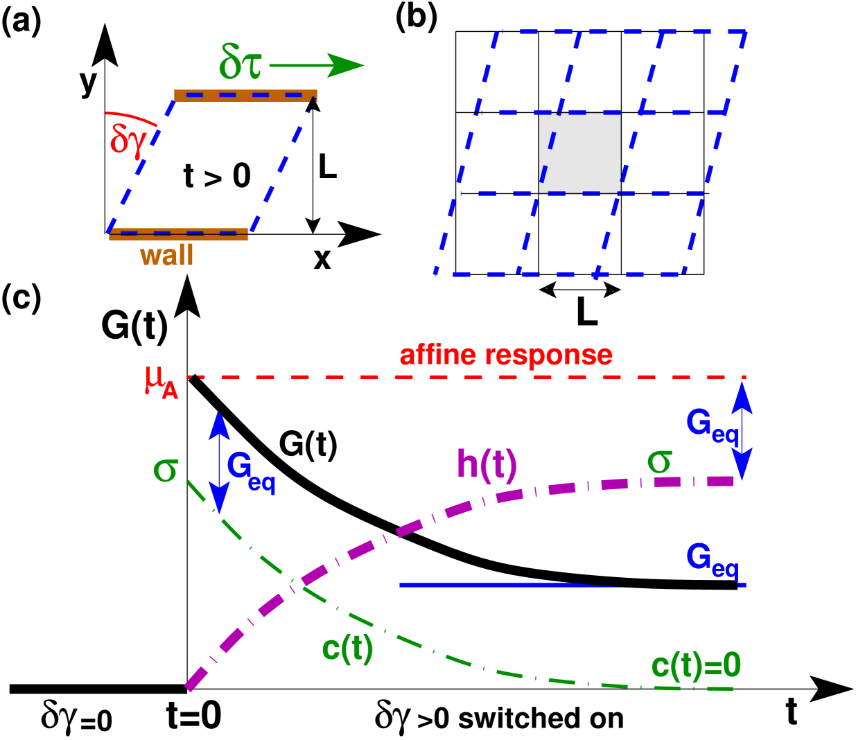
Figure 1: Notations and addressed problem: (a) experimental setup with $\delta\gamma$ being the shear strain, $\delta\tau$ the shear stress increment and $L$ the system size, (b) affine plain shear with periodic boundary conditions, (c) sketch of Eq. (2) and Eq. (3) with $G(t)$ being the response modulus (bold solid line), $G_{\mathrm{eq}}$ the equilibrium shear modulus (thin solid horizontal line), $\mu_{\mathrm{A}}$ the affine shear-elasticity (thin dashed horizontal line), $\sigma$ the shear-stress fluctuations, $c(t)$ the ACF (thin dash-dotted line) and $h(t)=\sigma-c(t)$ the MSD (bold dash-dotted line).

I Introduction

Background.

A central rheological property characterizing the linear response of (visco)elastic bodies is the shear relaxation modulus $G(t)$ Rubinstein and Colby (2003); Witten and Pincus (2004); Doi and Edwards (1986). Assuming for simplicity an isotropic body, $G(t)=\delta\tau(t)/\delta\gamma$ may be obtained from the stress increment $\delta\tau(t)$ after a small step strain $\delta\gamma$ has been imposed at time $t=0$ as sketched in panel (a) of Fig. 1. The instantaneous shear stress $\hat{\tau}(t)$ may be determined in a numerical study, as shown in panel (b) for a sheared periodic simulation box, from the model Hamiltonian and the particle positions and momenta Allen and Tildesley (1994). The long-time response yields the equilibrium shear modulus $G_{\mathrm{eq}}=\lim_{t\to\infty}G(t)$ as shown in panel (c). More readily, one may obtain $G_{\mathrm{eq}}$ by means of equilibrium simulations performed at constant volume $V$ and shear strain $\gamma$ using the stress-fluctuation relation Squire et al. (1969); Barrat et al. (1988); Barrat (2006); Lutsko (1989); Flenner and Szamel (2015); Wittmer et al. (2013); Wittmer et al. (2015a, b)

$$G_{\mathrm{eq}}=g\equiv\mu_{\mathrm{A}}-\sigma$$ (1)

with $\mu_{\mathrm{A}}$ being the “affine shear-elasticity” Wittmer et al. (2013); Wittmer et al. (2015a, b), a simple average characterizing the second order energy change under a canonical-affine shear strain Wittmer et al. (2015b). The second contribution $\sigma\equiv\beta V\langle\delta\hat{\tau}^{2}\rangle=\tilde{\sigma}-\sigma_{\star}$ stands for the rescaled shear stress fluctuation with $\beta$ being the inverse temperature and where we have introduced for later convenience the two terms $\tilde{\sigma}\equiv\beta V\langle\hat{\tau}^{2}\rangle$ and $\sigma_{\star}\equiv\beta V\langle\hat{\tau}\rangle^{2}$. As shown in Refs. Wittmer et al. (2013); Wittmer et al. (2015a, b) Eq. (1) can be derived using the general transformation relation for fluctuations between conjugated ensembles Lebowitz et al. (1967). Using these transforms for the shear-stress autocorrelation function (ACF) $c(t)\equiv\beta V\left<\delta\hat{\tau}(t)\delta\hat{\tau}(0)\right>\equiv\tilde{c}(t)-\sigma_{\star}$, Eq. (1) can be extended into the time domain Wittmer et al. (2015a, b). This allows the determination of the shear relaxation modulus using

$$G(t)=G_{\mathrm{eq}}+c(t)$$ (2)

as illustrated by the thin dash-dotted line in panel (c). Note that Eq. (2) is more general than the relation $G(t)=\tilde{c}(t)$ commonly used for liquids Doi and Edwards (1986); Hansen and McDonald (2006); Klix et al. (2012); Flenner and Szamel (2015). One important consequence of Eq. (2) is that a finite shear modulus $G_{\mathrm{eq}}$ is only probed by $G(t)$ on time scales where $c(t)$ actually vanishes. While $G_{\mathrm{eq}}$ can be obtained from Eq. (1), this is not possible using only $c(t)$ or $\tilde{c}(t)$ Wittmer et al. (2015a).

Key points made.

Note that both Eq. (1) and Eq. (2) assume that the sampling time $\Delta t$ is much larger than the longest, terminal relaxation time $t_{\star}$ of the system and that, hence, time and ensemble averages are equivalent. Since both relations are formulated in terms of fluctuating properties, not in terms of “simple averages” Allen and Tildesley (1994), this suggests that they might converge slowly with increasing $\Delta t$ to their respective thermodynamic limits. The aim of the present study is to rewrite and generalize (where necessary) both relations in terms of simple averages allowing an accurate determination even for $\Delta t\ll t_{\star}$. As we shall demonstrate this can be achieved by rewriting Eq. (2) simply as

$$G(t)=\mu_{\mathrm{A}}-\tilde{\sigma}+\tilde{c}(t)=G(0)-h(t)$$ (3)

with $G(0)=\mu_{\mathrm{A}}$ and $h(t)=\beta V/2\ \langle(\hat{\tau}(t)-\hat{\tau}(0))^{2}\rangle$ being the shear-stress mean-square displacement (MSD). We have used in the second step of Eq. (3) the exact identity

$$h(t)=\tilde{c}(0)-\tilde{c}(t)=c(0)-c(t)$$ (4)

with $\tilde{c}(0)=\tilde{\sigma}$ and $c(0)=\sigma$. Both expressions given in Eq. (3) are numerically equivalent $\Delta t$-independent simple averages.

Outline.

We begin by presenting in Sec. II the numerical model and remind some properties of the specific elastic network investigated already described elsewhere Wittmer et al. (2015a, b). Our numerical results are then discussed in Sec. III. Carefully stating the subsequent time and ensemble averages performed we present in Sec. III.1 the pertinent static properties as a function of the sampling time $\Delta t$. We emphasize in Sec. III.2 that the MSD $h(t)$ is a simple average not explicitly depending on the sampling time and on the thermodynamic ensemble. It will be demonstrated that our key relation Eq. (3) is a direct consequence of this simple-average behavior. We shall then turn in Sec. III.3 to the scaling of the ACF $c(t)$. We come back to the $\Delta t$-dependence of some static properties in Sec. III.4 where we compare several methods for the computation of $G_{\mathrm{eq}}$. Our work is summarized in Sec. IV where we discuss some consequences for the liquid limit and outline finally how Eq. (3) may be adapted for more general response functions.

II Some algorithmic details

Model Hamiltonian.

As in previous work Wittmer et al. (2013); Wittmer et al. (2015a, b) we illustrate the suggested general relations by molecular dynamics (MD) simulations Allen and Tildesley (1994) of a periodic two-dimensional network of ideal harmonic springs of interaction energy $\hat{\cal H}_{\mathrm{ex}}=\frac{1}{2}\sum_{l}K_{l}\left(r_{l}-R_{l}\right)^{2}$ with $K_{l}$ being the spring constant, $R_{l}$ the reference length and $r_{l}=|\underline{r}_{i}-\underline{r}_{j}|$ the length of spring $l$. (The sum runs over all springs $l$ between topologically connected vertices $i$ and $j$ of the network at positions $\underline{r}_{i}$ and $\underline{r}_{j}$.) The mass $m$ of the (monodisperse) particles and Boltzmann’s constant $k_{\rm B}$ are set to unity and Lennard-Jones (LJ) units are assumed throughout this paper.

Specific network.

As explained elsewhere Wittmer et al. (2013); Wittmer et al. (2015b) our network has been constructed using the dynamical matrix of a strongly polydisperse LJ bead glass quenched down to $T=0$ using a constant quenching rate and imposing a relatively large average normal pressure $P=2$. This yields systems of number density $\rho\approx 0.96$, i.e. linear length $L\approx 102.3$ for the periodic square box. Since the network topology is by construction permanently fixed, the shear response $G(t)$ must approach a finite shear modulus $G_{\mathrm{eq}}$ for $t\to\infty$ for all temperatures at variance to systems with plastic rearrangements. If not stated otherwise below, we use an $\text{NV}\gamma\text{T}$-ensemble with constant particle number $N=10^{4}$, volume $V=L^{2}$, shear strain $\gamma=0.00071$ foo (a) and temperature $T=1/\beta=0.001$. Due to the low temperature the ideal contributions to the average shear stress $\tau$ or the affine shear-elasticity $\mu_{\mathrm{A}}$ are negligible compared to the excess contributions. The static (ensemble averaged) thermodynamic properties of our finite-temperature network relevant for the present study are $P\approx 2$, $\tau\approx\sigma_{\star}\approx 0$, $\sigma\approx\tilde{\sigma}\approx 18$, $\mu_{\mathrm{A}}\approx 34$ and $G_{\mathrm{eq}}=\mu_{\mathrm{A}}-\sigma\approx 16$ as already shown elsewhere Wittmer et al. (2013); Wittmer et al. (2015b).

Technicalities.

As in Ref. Wittmer et al. (2015b) the data have been obtained using a Langevin thermostat of friction constant $\zeta=1$ and a tiny velocity-Verlet time step $\delta t_{\mathrm{MD}}=10^{-4}$. The instantaneous shear stress $\hat{\tau}$ and several other useful properties such as the instantaneous affine shear-elasticity $\hat{\mu}_{\mathrm{A}}$ Wittmer et al. (2015b) are written down every $10\delta t_{\mathrm{MD}}$ over several trajectories of length $t_{\mathrm{traj}}=10^{5}$. This is much larger than the longest stress relaxation time $t_{\star}\approx 10$ of the network properly defined in Sec. III.1. Packages of various sampling times $\Delta t\leq t_{\mathrm{traj}}$, as shown in Fig. 2, are then analyzed in turn using first time (gliding) averages within each package Allen and Tildesley (1994). Finally, we ensemble-average over different $\Delta t$-packages.

III Computational results

III.1 Sampling-time dependence of static properties

Notations.

A time average of a property $a$ within a $\Delta t$-package is denoted below by a horizontal bar, $\overline{a}$, and an ensemble average by $\langle a\rangle$. While “simple averages” of form $\langle\overline{a}\rangle$ generally do not depend on the sampling time, this may be different for averages of type $\langle\overline{a}^{2}\rangle$ and similar non-linear “fluctuations”. To mark this sampling time dependence we often note $\Delta t$ as an (additional) argument for the relevant property. Obviously, ergodicity implies $\overline{a}\to\langle a\rangle$ for large sampling times $\Delta t\gg t_{\star}$ for all properties considered. Hence, $\langle\overline{a}^{2}\rangle\to\langle\langle a\rangle^{2}\rangle=\langle a\rangle^{2}$, i.e. all $\Delta t$-effects must ultimately become irrelevant and the argument $\Delta t$ is dropped again to emphasize the thermodynamic limit.

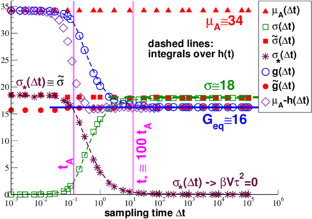
Figure 2: Sampling time dependence of various static properties. The “simple averages” $\mu_{\mathrm{A}}$, $\tilde{\sigma}$ and $\tilde{g}=\mu_{\mathrm{A}}-\tilde{\sigma}$ do not dependent on $\Delta t$ (filled symbols), while $\sigma_{\star}(\Delta t)$, $\sigma(\Delta t)$ and $g(\Delta t)$ do for $\Delta t\ll t_{\star}\approx 10\approx 100t_{\mathrm{A}}$. Only for $\Delta t\gg t_{\star}$ these “fluctuations” converge to their thermodynamic limits $\sigma_{\star}=0$, $\sigma\approx 18$ and $g=G_{\mathrm{eq}}\approx 16$. The dashed lines indicate for $\sigma_{\star}(\Delta t)$, $\sigma(\Delta t)$ and $g(\Delta t)$ the respective integrals over the MSD $h(t)$ according to Eq. (19). The diamonds represent $\mu_{\mathrm{A}}-h(t=\Delta t)$ ensemble-averaged over $10^{4}$ $\Delta t$-packages.

Simple averages.

We begin by verifying the (slightly trivial) $\Delta t$-dependence of the simple averages

$$\mu_{\mathrm{A}}(\Delta t) \equiv \left<\overline{\hat{\mu}_{\mathrm{A}}}\right>$$ (5)

$$\tilde{\sigma}(\Delta t) \equiv \beta V\left<\overline{\hat{\tau}^{2}}\right>$$ (6)

$$\tilde{g}(\Delta t) \equiv \mu_{\mathrm{A}}(\Delta t)-\tilde{\sigma}(\Delta t)$$ (7)

as shown in Fig. 2 (filled symbols). As expected, all three simple averages do indeed not depend on the sampling time and we shall drop below the argument $\Delta t$. We remind that according to the stress-fluctuation formula Eq. (1) $\mu_{\mathrm{A}}$ gives an upper bound for the shear-modulus $G_{\mathrm{eq}}$ Wittmer et al. (2013), while the rescaled second shear stress moment $\tilde{\sigma}$ gives the leading term to the shear-stress fluctuation $\sigma(\Delta t)$. Consistently with other work Barrat (2006); Wittmer et al. (2013) $\mu_{\mathrm{A}}$ is about twice as large as $\tilde{\sigma}$ and $\tilde{g}$ is thus finite. As can be seen, $\tilde{g}$ is essentially identical (for reasons given below) to the shear modulus $G_{\mathrm{eq}}\approx 16$ indicated by the bold solid line.

Fluctuations.

While the simple averages are $\Delta t$-independent, this is qualitatively different for the three “fluctuations”

$$\sigma_{\star}(\Delta t) \equiv \beta V\left<\overline{\hat{\tau}}^{2}\right>$$ (8)

$$\sigma(\Delta t) \equiv \tilde{\sigma}-\sigma_{\star}(\Delta t)$$ (9)

$$g(\Delta t) \equiv \mu_{\mathrm{A}}-\sigma(\Delta t)=\tilde{g}+\sigma_{\star}(\Delta t)$$ (10)

presented in Fig. 2 which reveal three distinct sampling time regimes. For very small $\Delta t\ll t_{\mathrm{A}}\approx 0.13$ (with $t_{\mathrm{A}}$ being properly defined below in Sec. III.2) the shear-stress fluctuations $\sigma(\Delta t)$ do naturally vanish since the instantaneous shear-stress $\hat{\tau}$ has no time to evolve and to explore the phase space. (There is no fluctuation for just one data entry.) Since $\sigma(\Delta t)\approx 0$, this implies that $\sigma_{\star}(\Delta t)\approx\tilde{\sigma}$ must have a constant shoulder and the same applies to the generalized stress-fluctuation formula $g(\Delta t)$, Eq. (10). The second time regime of about two orders of magnitude between $t_{\mathrm{A}}$ (left vertical line) and $t_{\star}\approx 10\approx 100t_{\mathrm{A}}$ (right vertical line) is due to the monotonous decay of $\sigma_{\star}(\Delta t)$, i.e. the ensemble averaged squared time-averaged shear stress indicated by stars. As a consequence, $\sigma(\Delta t)$ increases montonously in this interval while $g(\Delta t)$ decreases. The time scale $t_{\star}$ is the longest (terminal) time scale in this problem. Due to ergodicity time and ensemble averages become identical in the third sampling time regime for $\Delta t\gg t_{\star}$ where $\overline{\hat{\tau}}\to\langle\hat{\tau}\rangle=\tau$, $\sigma_{\star}(\Delta t)\to\beta V\tau^{2}$, $\sigma(\Delta t)\to\tilde{\sigma}-\beta V\tau^{2}$ and $g(\Delta t)\to g=G_{\mathrm{eq}}$ in agreement with the stress-fluctuation formula, Eq. (1).

Imposed zero average shear stress.

Since for convenience we have chosen $\tau=0$ for our network, this implies that $\sigma_{\star}(\Delta t)$ must vanish and in turn that $\sigma(\Delta t)\to\tilde{\sigma}$ and $g\to\tilde{g}$ as observed. It is thus strictly speaking due to the choice $\tau=0$, that the simple mean $\tilde{g}$ actually corresponds to the shear modulus $g=G_{\mathrm{eq}}$. For a more general imposed mean shear stress $\tau$ one might, however, readily use the shifted simple average

$$\tilde{g}\Rightarrow\tilde{g}+\beta V\tau^{2}=g=G_{\mathrm{eq}}$$ (11)

using the known/imposed (not the sampled) $\tau$ as a fast and reliable estimate of the shear modulus $G_{\mathrm{eq}}$ converging several orders of magnitude more rapidly than the classical (albeit slightly generalized) stress-fluctuation formula $g(\Delta t)$. We shall come back to the $\Delta t$-dependence of $\sigma_{\star}(\Delta t)$ and $g(\Delta t)$ in Sec. III.4.

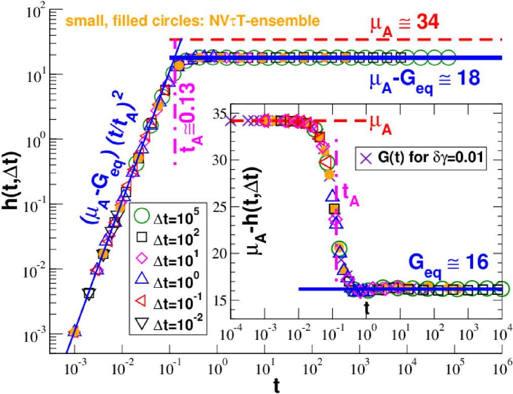
Figure 3: Shear-stress MSD $h(t,\Delta t)$ as a function of time $t$. The filled circles refer to $\text{NV}\tau\text{T}$-ensemble simulations for a sampling time $\Delta t=10^{3}$, all open symbols to the corresponding $\text{NV}\gamma\text{T}$-ensemble for a broad range of $\Delta t$. All data collapse. Main panel: The MSD increases as $h(t)\sim t^{2}$ for small times $t\ll t_{\mathrm{A}}$ (thin solid line) and becomes constant for $t\gg t_{\mathrm{A}}$ (bold solid line). The crossover time $t_{\mathrm{A}}\approx 0.13$ is obtained by matching both regimes. Inset: Comparison of $\mu_{\mathrm{A}}-h(t)$ with the shear-stress response function $G(t)$ obtained from the shear-stress increment $\left<\delta\hat{\tau}(t)\right>$ after applying a step-strain increment $\delta\gamma=0.01$ at $t=0$ (crosses).

III.2 Shear-stress mean-square displacement

$\Delta t$-independence.

The MSD $h(t,\Delta t)$ is presented in Fig. 3 as a function of time $t$ for a broad range of sampling times $\Delta t$. The data have been computed using

$$h(t,\Delta t)\equiv\frac{\beta V}{2}\left<\overline{\left(\hat{\tau}(t+t_{0})-\hat{\tau}(t_{0})\right)^{2}}\right>\mbox{ for }t\leq\Delta t$$ (12)

where the horizontal bar stands for the gliding average over $t_{0}$ within a $\Delta t$-package Allen and Tildesley (1994) and $\left<\ldots\right>$ for the final ensemble average over the packages. The first remarkable point in Fig. 3 is the perfect data collapse for all sampling times $\Delta t$, i.e. the MSD does not depend explicitly on $\Delta t$. This scaling is not surprising since $h(t,\Delta t)$ is a simple average measuring the difference of the shear stresses $\hat{\tau}(t+t_{0})$ and $\hat{\tau}(t_{0})$ along the trajectory and increasing $\Delta t/\delta t_{\mathrm{MD}}$ only improves the statistics but does not change the expectation value. The second argument $\Delta t$ is dropped from now on.

Ensemble-independence of MSD.

The small filled circles in Fig. 3 have been obtained for $\Delta t=10^{3}$ in the $\text{NV}\tau\text{T}$-ensemble at an imposed average shear stress $\tau=0$. An ensemble of $1000$ configurations with quenched shear strains $\hat{\gamma}$ distributed according to the $\text{NV}\tau\text{T}$-ensemble has been used Wittmer et al. (2015b); foo (b). All other data presented have been obtained in the corresponding $\text{NV}\gamma\text{T}$-ensemble foo (a). As already emphasized elsewhere Wittmer et al. (2015b), it is inessential in which ensemble we sample the MSD, i.e.

$$h(t)|_{\tau}=h(t)|_{\gamma}\mbox{ for }t\leq\Delta t.$$ (13)

The MSD $h(t)$ thus does not transform as a fluctuation, but as a simple average Allen and Tildesley (1994). Interestingly, assuming this fundamental scaling property one may (alternatively) demonstrate Eq. (3). To see this let us write down the exact identity Eq. (4) in the $\text{NV}\tau\text{T}$-ensemble

$$h(t)|_{\tau}=c(0)|_{\tau}-c(t)|_{\tau}=G(0)-G(t)$$ (14)

using in the last step that $G(t)=c(t)|_{\tau}$ foo (c) as shown by integration by parts in Eq. (15) of Ref. Wittmer et al. (2015a). Due to Eq. (13) and $G(0)=\mu_{\mathrm{A}}=\sigma|_{\tau}$ Wittmer et al. (2015a), this directly demonstrates $G(t)=\mu_{\mathrm{A}}-h(t)|_{\gamma}$ in agreement with Eq. (3). (For convenience $|_{\gamma}$ is dropped elsewhere.)

Time-dependence of MSD.

As seen from the main panel of Fig. 3, the MSD $h(t)$ of our extremely simple elastic network shows only two dynamical regimes. For small times $t\ll t_{\mathrm{A}}\approx 0.13$ the MSD increases quadratically as indicated by the thin solid line. This is to be expected if the MSD and/or the ACF are analytic around $t=0$ Wittmer et al. (2015b); Hansen and McDonald (2006). (Strictly speaking, this argument requires time-reversal symmetry, i.e. begs for an asymptotically small Langevin thermostat friction constant.) For larger times $h(t)$ becomes a constant given by $h(t)=\mu_{\mathrm{A}}-G_{\mathrm{eq}}=\sigma$ (bold solid line) in agreement with Eq. (3) and $G(t)\to G_{\mathrm{eq}}$ for $t\to\infty$. As seen in the main panel, the crossover time $t_{\mathrm{A}}$ is determined from the matching of both regimes. It marks the time where all forces created by an affine shear transformation have been relaxed by non-affine displacements Wittmer et al. (2015b).

Comparison with response function.

The key relation Eq. (3) is put to the test for all times $t$ in the inset of Fig. 3. We compare here $\mu_{\mathrm{A}}-h(t)$ obtained for different $\Delta t$ with the shear-stress response $G(t)$. The latter quantity has been computed from the shear-stress increment $\left<\delta\hat{\tau}(t)\right>$ with $\delta\hat{\tau}(t)\equiv\hat{\tau}(t)-\hat{\tau}(0^{-})$ measured after a step-strain $\delta\gamma=0.01$ has been applied at $t=0$. This is done using a metric-change of the periodic simulation box as illustrated in panel (b) of Fig. 1. As in Ref. Wittmer et al. (2015a) $\left<\delta\hat{\tau}(t)\right>$ has been averaged over $1000$ configurations. The perfect collapse of all data presented confirms the key relation and this for all sampling times $\Delta t$. This is the main computational result of the present work.

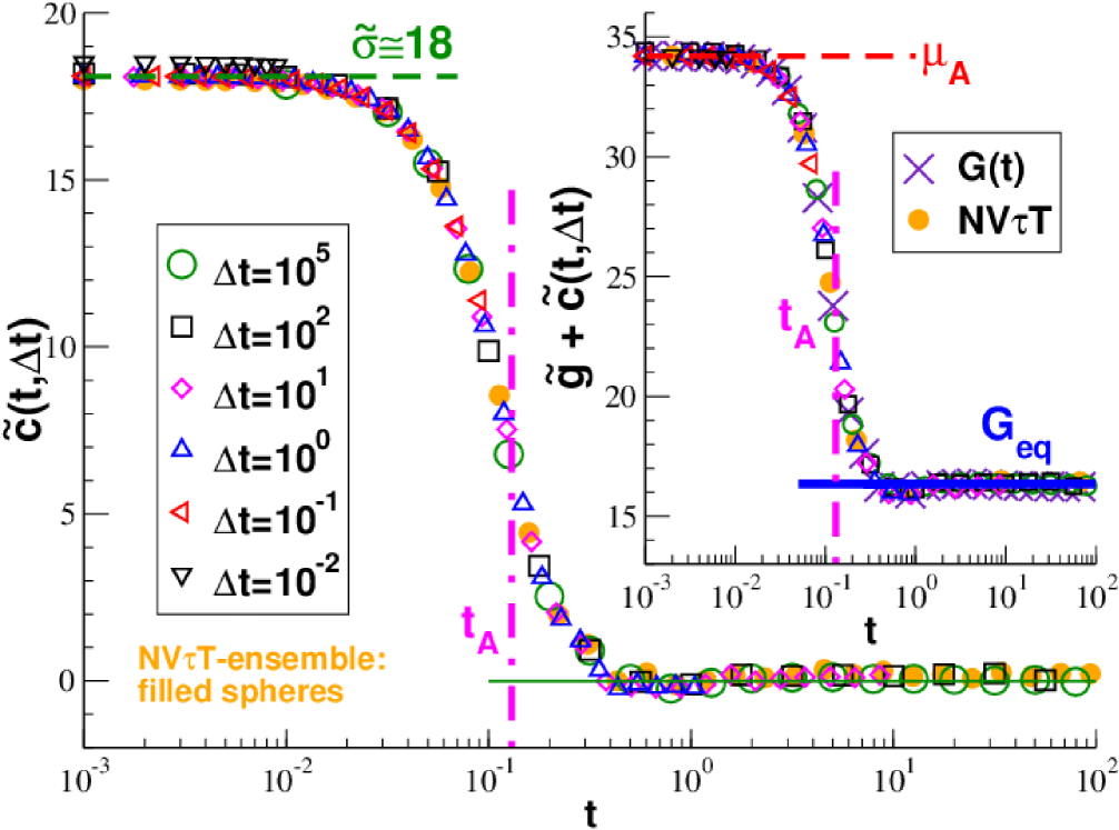
Figure 4: Shear-stress ACF $\tilde{c}(t,\Delta t)=\tilde{\sigma}-h(t,\Delta t)$ as a function of time $t$ for different sampling times $\Delta t$ as indicated. The filled spheres indicate results obtained in the $\text{NV}\tau\text{T}$-ensemble. As the MSD $h(t)$ the ACF $\tilde{c}(t)$ is a simple average neither depending on $\Delta t$ or the ensemble. Main panel: $\tilde{c}(t)\to\tilde{\sigma}$ for $t\to 0$ and $\tilde{c}(t)\to\sigma_{\star}=0$ for $t\gg t_{\mathrm{A}}$. Inset: Confirming Eq. (17) the shifted ACF $\tilde{g}+\tilde{c}(t)$ collapses perfectly on the directly measured response function $G(t)$.

III.3 Shear-stress autocorrelation function

We present in Fig. 4 the shear-stress ACF

$$\tilde{c}(t,\Delta t)\equiv\beta V\left<\overline{\hat{\tau}(t+t_{0})\hat{\tau}(t_{0})}\right>\mbox{ for }t\leq\Delta t$$ (15)

as a function of $t$ comparing different $\Delta t$ for the $\text{NV}\gamma\text{T}$-ensemble (open symbols) and one example with $\Delta t=10^{3}$ for the $\text{NV}\tau\text{T}$-ensemble (filled spheres). Since $\tilde{c}(t)=\tilde{\sigma}-h(t)$, this is essentially just a replot of the data already seen in Fig. 3 using, however, a more common representation. As one expects the ACF does depend neither on the sampling time nor on the ensemble, i.e. $\tilde{c}(t)$ is a simple average just as $h(t)$. Interestingly, by writing the identity Eq. (4) for the $\text{NV}\gamma\text{T}$-ensemble

$$h(t)|_{\gamma}=\tilde{c}(0)|_{\gamma}-\tilde{c}(t)|_{\gamma}=\tilde{\sigma}|_{\gamma}-\tilde{c}(t)|_{\gamma}$$ (16)

and using again Eq. (13) and Eq. (14) one verifies directly that within the $\text{NV}\gamma\text{T}$-ensemble

$$G(t) = \tilde{g}+\tilde{c}(t)$$ (17)

$$= g(\Delta t)+c(t,\Delta t)$$ (18)

holds where for convenience $|_{\gamma}$ has been dropped and the same notations $g(\Delta t)=\tilde{g}+\sigma_{\star}(\Delta t)$ are used as in Sec. III.1. Since $g(\Delta t)\to g=G_{\mathrm{eq}}$ for $\Delta t\gg t_{\star}$, Eq. (18) thus confirms Eq. (2) but generalizes it to finite sampling times $\Delta t$. As seen in the inset the response function $G(t)$ can be obtained by shifting $\tilde{c}(t)\to\tilde{g}+\tilde{c}(t)$ confirming thus Eq. (18). We emphasize that while $\tilde{c}(t)$ is a sampling-time independent simple average, the associated ACF $c(t,\Delta t)=\tilde{c}(t)-\sigma_{\star}(\Delta t)$ appearing in Eq. (16) and Eq. (18) is a fluctuation. It depends on the ensemble Wittmer et al. (2015a, b) and on the sampling time due to the substracted reference $\sigma_{\star}(\Delta t)$. It is simply for this reason that for $\Delta t\ll t_{\star}$, $c(t,\Delta t)$ is numerically less convenient than $\tilde{c}(t)$. However, for $\Delta t\gg t_{\star}$ both ACF become identical (not shown) since $\tilde{c}(t)\to\sigma_{\star}=\beta V\tau^{2}=0$ due to the zero average shear stress $\tau=0$ chosen.

III.4 Sampling-time effects revisited

We return now to the sampling-time behavior of the fluctuations $\sigma_{\star}(\Delta t)$, $\sigma(\Delta t)$ and $g(\Delta t)$ shown in Fig. 2. As seen, e.g., from Eq. (20) of Ref. Wittmer et al. (2015a), the $\Delta t$-effects can be understood by noticing that $\sigma(\Delta t)$ may be written as a weighted integral over the MSD $h(t)$ foo (d)

$$\sigma(\Delta t)=\frac{2}{\Delta t^{2}}\int_{0}^{\Delta t}\ \text{d}t\ (\Delta t-t)h(t).$$ (19)

Time translational invariance is assumed here and we have used that the MSD does not explicitly depend $\Delta t$. The sampling-time dependence of $\sigma(\Delta t)$ is thus reduced to the time dependence of $h(t)$. Equation (19) and the corresponding relations for $g(\Delta t)=\mu_{\mathrm{A}}-\sigma(\Delta t)$ and $\sigma_{\star}(\Delta t)=\tilde{\sigma}-\sigma(\Delta t)$ are indicated by thin dashed lines in Fig. 2. Also given is the simple-average expression $\mu_{\mathrm{A}}-h(t=\Delta t)$ for $\Delta t\leq 10^{2}$ (diamonds) using only the end-points of $\Delta t$-packages which are then in addition ensemble-averaged over $10^{4}$ independent packages. Since this corresponds to the response modulus $G(t)$ taken at $t=\Delta t$, it converges to $G_{\mathrm{eq}}$ already for sampling times $\Delta t\gg t_{\mathrm{A}}$, i.e. two orders of magnitude earlier than the stress-fluctuation formula $g(\Delta t)$ which only converges for $\Delta t\gg t_{\star}\approx 100t_{\mathrm{A}}$. The reason for this stems simply from the inequality

$$h(t=\Delta t)\geq\frac{2}{\Delta t^{2}}\int_{0}^{\Delta t}\ \text{d}t\ (\Delta t-t)h(t)$$ (20)

for a monotonously increasing function $h(t)$. Unfortunately, assuming the same number of $\Delta t$-packages, $\mu_{\mathrm{A}}-h(\Delta t)$ fluctuates much more strongly than $g(\Delta t)$, just as the end-to-end distance of a polymer chain fluctuates much more strongly as its radius of gyration. Equation (3) is thus only of interest for the determination of $G_{\mathrm{eq}}$ if a large ensemble of short trajectories with $t_{\mathrm{A}}\ll\Delta t\ll t_{\star}$ has been computed. As already pointed out in Sec. III.1, the most efficient property for the computation of the modulus is the simple average $\tilde{g}+\beta V\tau^{2}$. We note finally that since $h(t)$ is characterized by only one characteristic time, the crossover time $t_{\mathrm{A}}$, Eq. (19) implies that the terminal time $t_{\star}$ must be a unique function of $t_{\mathrm{A}}$ foo (e). Our simple network is thus only characterized by one characteristic time.

IV Conclusion

Summary.

Rewriting the central relation Eq. (2) of Ref. Wittmer et al. (2015a) it is shown that the shear-relaxation modulus $G(t)$ of an isotropic elastic body may be computed as $G(t)=\mu_{\mathrm{A}}-h(t)$ in terms of the difference of the two simple averages $\mu_{\mathrm{A}}$ and $h(t)$ characterizing, respectively, the canonical-affine strain response $G(0)$ at $t=0$ and the subsequent stress relaxation process for $t>0$. Interestingly, Eq. (2) and Eq. (3) may be directly demonstrated from the fundamental scaling $h(t)|_{\gamma}=h(t)|_{\tau}$ (Sec. III.2). Note that $G(t)=\mu_{\mathrm{A}}-h(t)$ and $G(t)=\tilde{g}+\tilde{c}(t)$ are equivalent simple-average expressions as shown, respectively in Fig. 3 and Fig. 4. From the practical point of view it is important that $h(t)$ or $\tilde{c}(t)$ do not depend explicitly on the sampling time $\Delta t$ and the response function $G(t)$ may thus be computed even if $\Delta t$ is much smaller than the terminal relaxation time $t_{\star}$ of the system. (For our simple networks $t_{\star}\approx 100t_{\mathrm{A}}$ with $t_{\mathrm{A}}$ being the crossover time of the MSD.) As shown in Sec. III.3, the relaxation modulus may be also obtained from the ACF $c(t,\Delta t)=\tilde{c}(t)-\sigma_{\star}(\Delta t)$ using $G(t)=g(\Delta t)+c(t,\Delta t)$ with $g(\Delta t)=\tilde{g}+\sigma_{\star}(\Delta t)$ being the generalized, sampling-time dependent stress-fluctuation estimate for the shear modulus $G_{\mathrm{eq}}$. For $\Delta t\gg t_{\star}$ these relations reduce to Eq. (2). Finally, comparing $\mu_{\mathrm{A}}-h(t\approx\Delta t)$ with the stress-fluctuation formula $g(\Delta t)$ it has been shown (Sec. III.4) that the former expression converges about two orders of magnitude more rapid, albeit with lesser accuracy depending on the number of independent $\Delta t$-packages used. The fastest convergence has been obtained, however, using the simple average $\tilde{g}+\beta V\tau^{2}$ (Fig. 2).

Discussion.

While the present paper has focused on solids, it should be emphasized that Eq. (3), being derived using quite general arguments not relying on a well-defined particle displacement field, should apply also to systems with plastic rearrangements and to the liquid limit. Due to its $\Delta t$-independence it should be useful especially for complex liquids and glass-forming systems Witten and Pincus (2004) with computationally non-accessible terminal relaxation times $t_{\star}$. We emphasize that the commonly used expression $G(t)=\tilde{c}(t)$ requires $\tilde{g}=\mu_{\mathrm{A}}-\tilde{\sigma}=0$ to hold foo (f). While this condition is justified for a liquid where $\tilde{g}=g=G_{\mathrm{eq}}=0$, it is incorrect in general as shown by the example presented in this work (Fig. 2). Hence, some care is needed when approximating $G(t)$ by $\tilde{c}(t)$ for systems below the glass transition Klix et al. (2012); Flenner and Szamel (2015). Since Eq. (3) can be used in any case and since it is not much more difficult to compute, it provides a rigorous alternative without additional assumptions Allen et al. (1994); foo (g).

Outlook.

Naturally, one expects that Eq. (3) can be generalized for more general linear relaxation moduli $M(t)$ of classical elastic bodies and fluids. With

$$M_{\mathrm{A}}=V\left<\left.\partial\hat{i}_{\beta}/\partial x_{\alpha}\right|_{x_{\alpha}x_{\beta}}\right>$$ (21)

characterizing the initial canonical-affine response $M(0)$ of the system to an infinitesimal change $\delta x_{\alpha}$ of an extensive variable $x_{\alpha}$ and $\delta i_{\beta}$ the subsequent change of an intensive system variable $i_{\beta}$ and

$$h(t)\equiv\frac{\beta V}{2}\left<\overline{\left(\hat{i}_{\alpha}(t)-\hat{i}_{\alpha}(0)\right)\left(\hat{i}_{\beta}(t)-\hat{i}_{\beta}(0)\right)}\right>$$ (22)

being the generalized MSD associated with the instantaneous intensive variables $\hat{i}_{\alpha}(t)$ and $\hat{i}_{\beta}(t)$, one expects $h(t)$ to be a simple average, i.e. $h(t)|_{x_{\alpha}x_{\beta}}=h(t)|_{i_{\alpha}i_{\beta}}$, and a generalized simple-average expression

$$M(t)=M(0)-h(t)\mbox{ with }M(0)=M_{\mathrm{A}}$$ (23)

should thus hold again. The reformulation of the general stress-fluctuation formalism in terms of such simple averages and the test of its computational efficiency are currently under way.