Polarimetric microlensing of circumstellar disks

Abstract

We study the benefits of polarimetry observations of microlensing events to detect and characterize circumstellar disks around the microlensed stars located at the Galactic bulge. These disks which are unresolvable from their host stars make a net polarization effect due to their projected elliptical shapes. Gravitational microlensing can magnify these signals and make them be resolved. The main aim of this work is to determine what extra information about these disks can be extracted from polarimetry observations of microlensing events in addition to those given by photometry ones. Hot disks which are closer to their host stars are more likely to be detected by microlensing, owing to more contributions in the total flux. By considering this kind of disks, we show that although the polarimetric efficiency for detecting disks is similar to the photometric observation, but polarimetry observations can help to constraint the disk geometrical parameters e.g. the disk inner radius and the lens trajectory with respect to the disk semimajor axis. On the other hand, the time scale of polarimetric curves of these microlensing events generally increases while their photometric time scale does not change. By performing a Monte Carlo simulation, we show that almost $4$ optically-thin disks around the Galactic bulge sources are detected (or even characterized) through photometry (or polarimetry) observations of high-magnification microlensing events during $10$ years monitoring of $150$ million objects.

1 Introduction

Gravitational microlensing is assigned to the increase in the brightness of a background star due to passing through the gravitational field of a foreground object Einstein (1936). Although this phenomenon was first proposed as a tool to probe the distribution and nature of dark matter in the Galactic disk Paczyński (1986), currently microlensing has been referred to a powerful method in detecting exo-planets, indicating the Galactic mass distribution, probing the stellar atmospheres , etc. (see e.g. Mao 2012, Gaudi 2012, Rahvar 2015). A significant problem in microlensing observations is that the number of the physical parameters of the source and lens is more than the number of the physical quantities measured from observations (see e.g. Kains et al. 2013). Hence, extra observational constraints are needed to resolve the lensing degeneracy.

A method for partially breaking the microlensing degeneracy and obtaining extra information about the lens or source star is performing astrometry or polarimetry observations in addition to the photometry observation. For example, the astrometric shift in the source trajectory due to the lensing effect (see e.g. Walker 1995, Høg et al. 1995) gives us the angular Einstein radius which by adding the parallax effect measurement, the lens mass can be inferred Paczyński (1997); Miralda-Escdé (1996); Rahvar et al. (2003). Polarimetric observations can also be done during microlensing events. Indeed, there is a local polarization over the star surface due to the photon scattering occuring in the stellar atmospheres. The effect is particularly effective for the host stars that have a free electron atmosphere Chandrasekhar (1960). By a minor extent, polarization may be also induced in main-sequence stars (of late-type) by the scattering of star light off atoms and molecules Fluri & Stenflo (1999) and in evolved, cool giant stars by photon scattering off dust grains contained in extended envelopes Simmons et al. (2002). However, the net polarization of a distant star is zero due to symmetric orientations of local polarizations on its surface with respect to the source centre. During a microlensing event, the circular symmetry of the source surface is broken which causes a net polarization from the source star Schneider & Wagoner (1987); Simmons et al. 1995a,b ; Bogdanov et al. (1996).

Polarimetry observations during microlensing events by partially resolving the microlensing degeneracy can help us to evaluate the finite source effect, the Einstein radius, the limb-darkening parameters of the source star and the lens impact parameter Yoshida (2006); Agol (1996); Schneider & Wagoner (1987); Simmons et al. (2002).

On the other hand, polarimetric microlensing can probe the surface and the atmosphere of the source stars by magnify the small polarization signals from the anomalies on the surface of stars such as stellar spots and magnetic fields to be detected Sajadian & Rahvar (2015); Sajadian 2015b . Another anomaly in the star atmosphere that makes a net polarization is the existence of a circumstellar disk around the source. Here, we study detecting and characterizing this anomaly through polarimetric microlensing.

Although $170$ disks have been resolved until now , most of them were located at distances less than $1$ kpc from us. Through gravitational microlensing, we can potentially detect and even characterize the circumstellar disks around the Galactic bulge stars. Hence, using this method we can study the environmental effects on the disks’ structure as well as statistically investigate them. Gravitational microlensing of (or due to) disks has been discussed in details by a number of authors, e.g. microlensing by lenses consisting of the gas clouds was first investigated by Bozza and Mancini (2002). Then, microlensing effects on a source surrounded by a circumstellar disk as a function of the wave length were studied by Zheng and Ménard (2005) and they showed that the magnification factors of these disks reach to $\mathrm{10\%-20\%}$ in the mid- and far- infrared. Recently, Hundertmak et al. (2009) investigated the microlensing as a tool for detecting debris disks around microlenses and estimated that one debris disk per year can be detected through microlensing. Another application of gravitational microlensing for detecting circumstellar disks around source stars is performing polarimetry observations.

In this work, we investigate detecting and characterizing circumstellar disks around source stars through polarimetry observations during microlensing events. Here, only optically-thin disks which contain hot circumstellar dusts and are located beyond the condensation radius $\mathrm{(\sim 1500K)}$ are considered. It seems that about $10\%$ of solar-type stars (G- and K-type) in our neighbourhood have such disks Absil et al. (2013); Ertel et al. (2014). Detecting this kind of disks even around nearby stars needs high-resolution observations with interferometers, because of small angular separation between the disk and the host star. In the direction of Galactic bulge for polarimetry microlensing, the late-type stars with disks around them are the most suitable sources for polarimetry observations. Our plan is also performing statistical study of these events. During the lensing of these sources, the closer distances from their host stars (small impact parameter) makes higher magnification factor as well as higher contributions in total Stokes parameters.

In section (2) we explain the formalism used to calculate the polarization of sources surrounded by circumstellar disks in microlensing events. The characteristics of the polarimetric microlensing of source stars with circumstellar disks are studied in section (3). In section (4) we evaluate the efficiencies of detecting disks around the source stars through polarimetry and photometry microlensing (in optical wavelength) by performing a Monte Carlo simulation. Finally, we give conclusions in the last section.

2 The formalism of polarimetric microlensing of disks

Here, we explain how to calculate the polarization in gravitational microlensing (the first subsection) and the polarization due to lensed source stars with circumstellar disks (the second subsection).

2.1 Polarimetry microlensing

The existence of a net polarization due to the lensing effect for supernovae was first pointed out by Schneider & Wagoner (1987). They analytically estimated the amounts of polarization degree near point and critical line singularities. The polarization during microlensing events was investigated by a number of authors Simmons et al. 1995a,b ; Bogdanov et al. (1996). Polarization in binary microlensing events was also numerically calculated by Agol (1996) and he noticed that in a binary microlensing event the net polarization is larger than the net polarization generated by a single lens and can reach to one per cent during the caustic-crossing. Polarization from microlensing of cool giants with spherically symmetric envelopes by a point lens and binary microlenses was investigated by Simmons et al. (2002) and Ignace et al. (2006). Ingrosso et al. (2012,2015) evaluated the expected polarization signals for a set of reported high-magnification single-lens and exo-planetary microlensing events as well as OGLE-III events towards the Galactic bulge. Recently, Sajadian and Rahvar (2015) noticed that there is an orthogonal relation between the polarization and astrometric shift of source star position in the simple and binary microlensing events except in the fold singularities and investigated the advantages of this correlation for studying the surface of a source star and spots on it.

To describe a polarized light, we use the Stokes parameters $\mathrm{S_{I}}$, $\mathrm{S_{Q}}$, $\mathrm{S_{U}}$ and $\mathrm{S_{V}}$. These parameters are, the total intensity, two components of linear polarizations and circular polarization over the source surface, respectively Tinbergen (1996). Taking into account that there is only linear polarization of light scattered on the atmosphere of a star, we set $\mathrm{S_{V}=0}$. Therefore, the polarization degree $(P)$ and angle of polarization $\mathrm{(\theta_{p})}$ as functions of total Stokes parameters are Chandrasekhar (1960):

$$P = \frac{\sqrt{S_{Q}^{2}+S_{U}^{2}}}{S_{I}},$$

$$\theta_{p} = \frac{1}{2}\tan^{-1}{\frac{S_{U}}{S_{Q}}}.$$ (1)

In microlensing events, the Stokes parameters are given by:

$$S_{I} = ~{}\rho^{2}_{\star}\int_{0}^{1}\rho~{}d\rho\int_{-\pi}^{\pi}d\phi I^{\star}(\mu)~{}A(u),$$ (2)

$$\left(\begin{array}[]{c}S_{Q}\\ S_{U}\end{array}\right) = \rho^{2}_{\star}\int_{0}^{1}\rho~{}d\rho\int_{-\pi}^{\pi}d\phi I^{\star}_{-}(\mu)A(u)\left(\begin{array}[]{c}-\cos 2\phi\\ \sin 2\phi\end{array}\right),$$ (6)

where $\mathrm{\rho}$ is the distance from the center to each projected element over the source surface normalized to the projected radius of star on the lens plane (i.e. $\mathrm{\rho_{\star}}$), $\mathrm{\mu=\sqrt{1-\rho^{2}}}$, $\mathrm{\phi}$ is the azimuthal angle between the lens-source connection line and the line from the center to each element over the source surface, $\mathrm{u=(u_{cm}^{2}+\rho^{2}\rho^{2}_{\star}-2\rho\rho_{\star}u_{cm}\cos\phi)^{1/2}}$ is the distance of each projected element over the source surface with respect to the lens position, $\mathrm{u_{cm}}$ is the impact parameter of the source center and $A(u)$ is the magnification factor.

$\mathrm{I^{\star}(\mu)}$ and $\mathrm{I^{\star}_{-}(\mu)}$ are the total and polarized light intensities that depends on the type of the source star. Different physical mechanisms for various types of stars make the overall polarization signals Ingrosso et al. (2012). For instance, in the hot early-type stars, the electron scattering in their atmosphere produces the polarization signal. The amounts of Stokes intensities over the surface of these stars were first evaluated by Chandrasekhar (1960) and then their numerical amounts were approximated by the following functions Schneider & Wagoner (1987):

$$I^{\star}(\mu) = I_{0}(1-c_{1}(1-\mu)),$$

$$I^{\star}_{-}(\mu) = I_{0}c_{2}(1-\mu),$$ (7)

where $\mathrm{c_{1}=0.64}$, $\mathrm{c_{2}=0.032}$ and $\mathrm{I_{0}}$ is the source intensity in the line of sight direction. For late-type main-sequence stars, the polarization signal is produced because of both Rayleigh scattering on neutral hydrogens and with a minor contribution from the Thompson scattering by free electrons Fluri & Stenflo (1999). The amount of polarization degree for this kind of stars was approximated as follows Stenflo (2005):

$$P(\mu)=q_{\lambda}\frac{1-\mu^{2}}{(\mu+m_{\lambda})(I_{\lambda}(\mu)/I_{\lambda}(1))},$$ (8)

where $\mathrm{I_{\lambda}(\mu)/I_{\lambda}(1)}$ shows the center-to-limb variation of the intensity, $\mathrm{q_{\lambda}}$ and $\mathrm{m_{\lambda}}$ are linear functions of wavelength (see more details in Ingrosso et al. 2012). Finally, in cool giant stars Rayleigh scattering on atomic and molecular species or on dust grains generates the polarization signal. In this regard, Simmons et al. (2002) offered the relevant Stokes parameters for giant stars with spherically circumstellar envelopes lensed by a single lens.

2.2 Polarization due to circumstellar disks

We assume that there is a circumstellar disk around the source star. A disk has mostly a circular shape with respect to its host star, while its projected shape on the sky plane is generally an ellipse. Hence, the projection breaks the circular symmetry and the result is a net polarization. Gravitational lensing of the star surrounded by such a disk can magnify the disk polarization signal, change its orientation and make it be detected. The amount of magnified polarization depends on the orientation of disk with respect to the lens trajectory as well as the disk structure and its projected surface density.

Here we use some parameters to quantify a circumstellar disk around the source star in our calculation as: (i) the inner and outer radii $\mathrm{R_{i}}$, $\mathrm{R_{o}}$ (here, we define the disk inner radius beyond the source condensation radius where the dust forms and the outer radius of the disk where its Stokes intensities with respect to the source intensity decrease significantly e.g. by four orders of magnitude), (ii) the inclination angle $i$ to project the disk on the sky plane, i.e. the angle between the normal to disk and the line of sight towards the observer and (iii) some parameters to indicate the disk density distribution: the length scale $\mathrm{R_{c}}$ where the electron number density of the disk in the mid plane reaches to $\mathrm{n_{0}}$ (here we set $\mathrm{R_{c}=R_{i}}$), $\mathrm{\gamma}$ and $\mathrm{\beta}$ which specify the radial dependence of the disk surface density and its thickness respectively, $\mathrm{R_{s}}$ and $\mathrm{h_{0}}$ which indicate the thickness of the disk versus the radial distance in the mid plane. The more details about the disk density distribution can be found in the Appendix (B).

We also assume some limitations to model the Stokes intensities of the disk: (i) the disk has a circular shape in the stellar coordinate system, (ii) the disk is optically thin, (iii) The scattering opacity which produces the polarization for the disk is the photon scattering on atomic and molecular species (Rayleigh scattering) or on the dust grains, (iv) the magnetic field of the disk is negligible, (v) the incident radiation of the source star to the disk is unpolarized, (vi) any diffuse contribution from other parts of the disk is not included, (vii) the single scattering approximation is used and (viii) the disk inner radius is beyond of the condensation radius.

Let us characterize the lens plane by $\mathrm{(x,y)}$ axes and put the projected center of source at the center of coordinate system so that $\mathrm{x}$-axis is parallel with the semimajor axis of the disk (after projection on the sky and lens planes), $\mathrm{y}$-axis is normal to it and $\mathrm{z}$-axis is toward the observer (see Figure 3). We normalize all parameters to the Einstein radius of the lens, $\mathrm{R_{E}}$. Generally, the projected disk on the sky plane has an elliptical shape that the ratio of its minor to major axes is $\mathrm{\cos(i)}$. The positions of the lens and each element of the projected disk in this reference frame normalized to $\mathrm{R_{E}}$ are $\mathrm{(x_{l},y_{l})}$ and $\mathrm{(x_{d},y_{d})=(\varrho\cos\varphi,\varrho\sin\varphi)}$ where $\mathrm{\varphi}$ alters in the range of $\mathrm{[0,2\pi]}$ and $\mathrm{\varrho}$ changes in the range of $\mathrm{\varrho\in[\varrho_{i},\varrho_{o}](1+\sin^{2}\varphi\tan^{2}i)^{-1/2}}$ Zheng & Ménard (2005), $\mathrm{\varrho_{i}=R_{i}x_{ls}/R_{E}}$ and $\mathrm{\varrho_{o}=R_{o}x_{ls}/R_{E}}$ where $\mathrm{x_{ls}=D_{l}/D_{s}}$ the ratio of the lens and the source distances from the observer. Indeed, we choose a circular disk around the source star before projecting on the sky plane.

To calculate the overall Stokes parameters, we should add the contributions of the source and its disk as follows:

$$\left(\begin{array}[]{c}S^{\prime}_{I}\\ S^{\prime}_{Q}\\ S^{\prime}_{U}\end{array}\right) = \left(\begin{array}[]{c}S_{I}\\ S_{Q}\\ S_{U}\end{array}\right)$$ (15)

$$+ \int_{0}^{2\pi}~{}d\varphi~{}\int_{\varrho_{i}}^{\varrho_{o}}~{}\varrho~{}d\varrho~{}A(u_{d})\boldsymbol{I}_{d}(\varrho,\varphi),$$ (16)

where $\mathrm{S_{I}}$, $\mathrm{S_{Q}}$ and $\mathrm{S_{U}}$ are the Stokes parameters due to the source given by equation (2) and the second term calculates the disk Stokes parameters. $\mathrm{u_{d}=\sqrt{(x_{d}-x_{l})^{2}+(y_{d}-y_{l})^{2}}}$ is the distance of each projected element of the disk from the lens position. Integrating is done over the disk area projected on the lens plane. $\mathrm{\boldsymbol{I}_{d}(\varrho,\varphi)}$ as a vector contains the Stokes intensities of the disk in the observer coordinate system. More details about calculating these Stokes intensities by considering the mentioned limitations are brought in the Appendix (A).

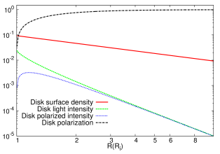
Figure 1: The surface density (normalized to the amount of $n_{0}$) (red solid line), light intensity (green dashed line), polarized intensity (blue dotted line) and polarization signal (black dot-dashed line) of the disk are plotted versus the normalized distance started from the disk inner radius. Here, we assume that the disk and central star intensities are resolvable, so that we mask the central star and consider only the light and polarized intensities from the disk to calculate the polarization degree. Here, we set $\mathrm{\gamma=9/4}$, $\mathrm{\beta=5/4}$, $\mathrm{h_{0}=10AU}$, $\mathrm{R_{c}=R_{i}=R_{\star}}$, $\mathrm{R_{s}=100AU}$, $\mathrm{I_{0}=1}$ and $\mathrm{\tau_{eq}=1}$.

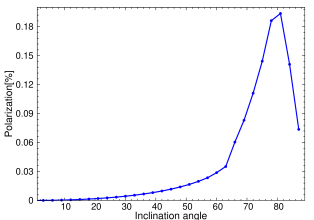
Figure 2: The total polarization signal owing to a source star with the circumstellar disk characterized in Figure (1) without lensing effect versus the disk inclination angle.

Here, we study the disk polarization signal without considering the lensing effect. In Figure (1) we plot the surface density (red solid line), light intensity (green dashed line), polarized intensity (blue dotted line) and polarization degree (black dot-dashed line) of a typical disk versus the normalized distance started from the inner radius of disk. The parameters used to make this figure are $\mathrm{\gamma=9/4}$, $\mathrm{\beta=5/4}$, $\mathrm{h_{0}=10AU}$, $\mathrm{R_{s}=100AU}$, $\mathrm{I_{0}=1}$, $\mathrm{R_{c}=R_{i}=R_{\star}}$ where $\mathrm{R_{\star}}$ is the source radius. Note that we normalize the disk surface density to the amount of $\mathrm{n_{0}}$ (whose definition is brought in equation 38) to justify its range with the ranges of the light and polarized intensities. As explained in the Appendix (B), the polarization signal due to the disk is proportional to the equatorial optical depth due to the dust scattering, i.e. $\mathrm{\tau_{eq}}$, whose definition is brought in the equation (39). Here we set $\mathrm{\tau_{eq}=1}$. Here, we assume that the disk and the central star intensities are resolvable, so that we mask the central star and consider only the light and polarized intensities from the disk for calculating the polarization degree. The light intensities as well as the disk surface density decrease by increasing the distance from the source star. The disk polarized light is maximized at almost the disk inner radius. Hence, during lensing if the lens crosses the disk inner radius the polarimetric disk-induced perturbation maximizes.

If the source is so far from us, we can not discern the source light from the disk light and receive the total polarization signal due to the disk and its central star. If there is no lensing effect, the total polarization signal depends strongly on the projected shape of the disk which is a function of the disk inclination angle as well as the dust optical depth of the disk. In Figure (2) we plot the total polarization signal of the source star surrounded by the circumstellar disk (specified in Figure 1) versus the disk inclination angle. The more inclined disks, the higher polarization signals. However, the maximum polarization signal happens for the disks with the inclination angles between $\mathrm{70^{\circ}-80^{\circ}}$ which agrees with the results of simulations of polarization signals for gaseous disks around Be-stars (see e.g. Halonen et al. 2013, Halonen and Jones 2013). The polarization angle of different inclined disks does not depend on the disk inclination angle in contrast with the polarization degree. Because, an inclined disk has a symmetric density distribution with respect to its semiminor and major axes. Hence, the disk Stokes parameter $\mathrm{S_{U}}$ vanishes and $\mathrm{S_{Q}}$ becomes negative which result the polarization angle equal to $90$ with respect to its semimajor axis (see equation 2.1).

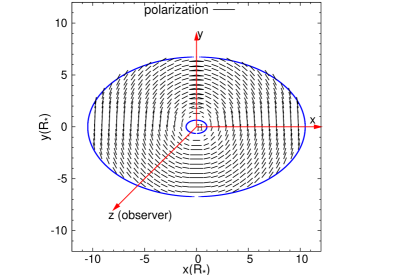
Figure 3: The polarization map around that disk specified in Figure (1) with the inclination angle $\mathrm{i=50^{\circ}}$. The size of lines is proportional to the polarization degree.

In Figure (3) we plot the polarization map over that disk with the inclination angle $\mathrm{i=50^{\circ}}$. Note that, the size of lines is proportional to the polarization degree. The polarization orientation (i.e. $\mathrm{\theta_{p}}$) is given in terms of its angle with respect to $\mathrm{x}$-axis. The largest polarization signals occur near the disk outer radius whereas the maximum polarized intensity comes from the disk inner radius. Having simulated a circumstellar disk around the source star, we turn on the lensing effect and study detecting disks through polarimetric microlensing which is explained in the following section.

3 Polarimetric microlensing of disks

In this section, we study the characteristics of polarimetric curves of lensed source stars with circumstellar disks. In Figure (4) some polarimetry and photometry curves due to microlensing events of source stars surrounded by circumstellar disks are represented. According to these Figures, we notice some significant properties of light and polarimetric curves as following. In this section, we consider early-type stars in the microlensing sources and use equations (2.1) to calculate the source Stokes intensities.

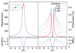
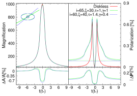
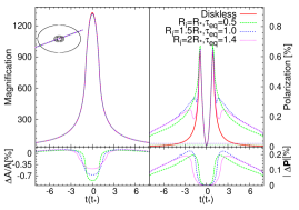
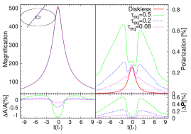
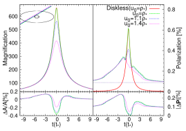
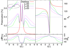
Figure 4: Example polarimetric microlensing events affected with a circumstellar disk around the source star. In each subfigure, the light and polarimetric curves are shown in left and right panels. The source (grey circle) with circumstellar disk (black ellipses) projected on the lens plane and lens trajectory are shown with insets in the left-hand panels. The simple models without disk effect are shown by red solid lines. The thinner straight lines in right panels represent the polarization signal of disk without lensing effect. The photometric and polarimetric residuals with respect to the simple models are plotted in bottom panels. Noting that, in the last panel (f), the curves of polarization degree and its angle during a microlensing event with three different amounts of $\mathrm{\xi}$ are shown instead of light and polarimetric curves. The parameters used to make these figures can be found in Table (1). We also set $\mathrm{M_{l}=0.3~{}M_{\odot}}$, $\mathrm{D_{l}=6.5~{}kpc}$, $\mathrm{D_{s}=8~{}kpc}$, $\mathrm{R_{c}=R_{i}}$, $\mathrm{h_{0}=10~{}AU}$, $\mathrm{R_{s}=100~{}AU}$ and the limb-darkening coefficients over the source surface $\mathrm{c_{1}=0.64}$ and $\mathrm{c_{2}=0.032}$.

(a) The time scale of the polarimetric curve of the lensed source star surrounded by a circumstellar disk increases. This time scale depends on (i) the disk density distribution which indicates the disk equatorial optical depth and (ii) the disk and lens geometrical parameters, e.g. the angle of the lens-source trajectory with respect to the disk semimajor axis $\mathrm{\xi}$ and the disk inclination angle. The disk length that lens crosses with the impact parameter $\mathrm{u_{0}}$ is given by:

$$\Delta L=\frac{2}{f^{2}}\sqrt{\varrho^{2}_{o}f^{2}-u^{2}_{0}(1+\tan^{2}i)},$$ (17)

where $\mathrm{f=\sqrt{1+\sin^{2}\xi\tan^{2}i}}$. Examples of these lengths are shown in the inset in the left-hand panel of Figure 4 in which the ellipse shows the projected outer radius of the disk and the straight lines represent the lens trajectories with the different angles with respect to the disk semimajor axis. Let us assume $\mathrm{\varrho_{o}\sim 5\rho_{\star}}$ the distance from the source star in which the polarized intensity of the disk with $\mathrm{\tau_{eq}=1}$ almost decreases by four orders of magnitude with respect to the source intensity (according to Figure 1). By considering high-magnification microlensing events with $\mathrm{u_{0}\leq\rho_{\star}}$ in which the probability of detecting the polarization signals due to the lensed sources is high, we calculate the average amount of the time duration when the lens crosses the disk length which is $\mathrm{\bar{\Delta t}=\bar{\Delta L}\times t_{E}\sim 8t_{\star}}$. Here $\mathrm{t_{E}}$ is the Einstein crossing time and $\mathrm{t_{\star}=\rho_{\star}t_{E}}$ is the time of crossing the projected source radius which is the time scale of a typical polarimetric microlensing without any perturbation. Noting that $\mathrm{\bar{\Delta L}}$ is a dimensionless parameter. Therefore, the time scale of the polarimetric microlensing of the source surrounded by the disk with $\mathrm{\tau_{eq}=1}$ increases in averagely by one order of magnitude with respect to that without disk effect. If the disk equatorial optical depth decreases, the outer radius of the disk shrinks. As a result, the increase in the polarimetric time scales lessens by decreasing the disk equatorial optical depth. Increasing in the time scale also occurs in the polarimetric microlensing events of cool giant stars with spherically symmetric envelopes Simmons et al. (2002). We note that the time scale of light curves of these microlensing events does not significantly change in contrast with the polarimetric ones.

	Figure number	$M_{\star}(M_{\odot})$	$R_{\star}(R_{\odot})$	$T_{\star}(K)$	$\rho_{\star}\times 10^{3}$	$R_{i}(R_{\star})$	$R_{o}(R_{\star})$	$\tau_{eq}$	$i^{\circ}$	$\gamma$	$u_{0}(\rho_{\star})$	$\xi^{\circ}$
	$4(a)$	$0.6$	$0.66$	$3796$	$1.5$	$1$	$10.5$	$1$	$65$	$1.0$	$0$	$--$
	$4(b)$	$1.0$	$1.0$	$5770$	$2.2$	$1$	$5.5$	$--$	$--$	$--$	$0.1$	$--$
	$4(c)$	$0.7$	$0.75$	$4191$	$1.6$	$--$	$8.5$	$--$	$50$	$1$	$0.1$	$20$
	$4(d)$	$0.7$	$0.75$	$4191$	$1.6$	$2$	$10.5$	$--$	$60$	$1$	$1.3$	$50$
	$4(e)$	$0.8$	$0.83$	$4719$	$1.8$	$1.5$	$9.5$	$1.1$	$70$	$1$	$--$	$30$
	$4(f)$	$0.7$	$0.75$	$4191$	$1.6$	$2$	$10.5$	$0.3$	$70$	$1$	$0.6$	$--$

Table 1: The table contains the parameters used to make microlensing events shown in Figures 4, 4, 4, 4, 4 and 4. These parameters are the source mass $\mathrm{M_{\star}(M_{\odot})}$, the source radius $\mathrm{R_{\star}(R_{\odot})}$, the photosphere temperature of the source $\mathrm{T_{\star}(K)}$, the projected source radius in the lens plane, normalized to the Einstein radius $\mathrm{\rho_{\star}(\times 10^{3})}$, the disk inner radius normalized to the source radius $\mathrm{R_{i}(R_{\star})}$, the normalized outer radius of the disk $\mathrm{R_{o}(R_{\star})}$, the disk equatorial optical depth $\mathrm{\tau_{eq}}$, the inclination angle of the disk $\mathrm{i^{\circ}}$, $\mathrm{\gamma}$ which indicates the radial dependence of disk density distribution, the impact parameter of the source center normalized to $\mathrm{\rho_{\star}}$ $\mathrm{u_{0}(\rho_{\star})}$ and the angle of the lens trajectory with respect to the disk semimajor axis $\mathrm{\xi^{\circ}}$ respectively. For these figures, we also set the mass of the primary lens $\mathrm{M_{l}=0.3~{}M_{\odot}}$, the lens and source distance from the observer $\mathrm{D_{l}=6.5~{}kpc}$ and $\mathrm{D_{s}=8.0~{}kpc}$ and the limb-darkening coefficients $\mathrm{c_{1}=0.64}$ and $\mathrm{c_{2}=0.032}$.

Figure 4 shows a polarimetric microlensing event of a source star with a circumstellar disk, considering three different amounts of $\mathrm{\xi}$. Photometry and polarimetry curves are shown in the left and right panels. The source star (grey circle), its circumstellar disk (black ellipses) projected on the lens plane and the lens trajectory are shown with an inset in the left-hand panel. The simple models without disk effect are shown by red solid lines. The thinner straight lines in the right panels represent the polarization signal of the disk without lensing effect. The photometric and polarimetric residuals with respect to the simple models are plotted in the bottom panels. The polarimetric residual is the residual in the polarization vector i.e.

$$\mathrm{|\boldsymbol{\Delta P}|=\sqrt{P^{\prime 2}+P^{2}-2P^{\prime}P\cos 2(\theta^{\prime}_{p}-\theta_{p})},}$$

where the prime symbol refers to the related quantity considering the disk effect. The parameters used to generate these microlensing events can be found in Table (1). For the case that lens trajectory is parallel with the semimajor axis of the disk, the polarimetry curve has the longest time scale.

The polarization angle of an inclined disk without lensing effect is $\mathrm{90^{\circ}}$ with respect to its semimajor axis. Whereas, the polarization signal of the source is always normal to the lens-source connection line (see e.g. Sajadian and Rahvar 2015). When the lens is entering into an inclined disk normal to the disk semimajor axis $\mathrm{(\xi=90^{\circ})}$, the polarizations of the disk and source are normal to each other. In that case as the lens is moving towards the source center, at some time these two polarization signals will have the same amounts and the total polarization signal vanishes which is shown in Figure 4. When $\mathrm{\xi=0^{\circ}}$, the polarization signals due to the source and disk are always parallel and as a result enhances each other. Hence, as the lens is entering the disk parallel with the disk semimajor axis the total polarization signal is always enhancing (see Figure 4). Detecting these features in the polarimetric curves of the microlensing events helps us to evaluate the angle of the lens-source trajectory with respect to the disk semimajor axis i.e. $\mathrm{\xi}$. Noting that the variation of $\mathrm{\xi}$ has no detectable effect on the light curves and the photometric residuals are similar for different values of $\mathrm{\xi}$. Hence, the polarimetry observations of microlensing events can give some information about the disk geometrical structure.

If the impact parameter of the lens trajectory is small $\mathrm{u_{0}\sim 0}$, the polarimetry and photometry curves almost have symmetric shapes with respect to the time of the closest approach. Because, the disk surface density is symmetric with respect to the semimajor and minor axes (see Figure 4). However, due to the projection process, if $\mathrm{\varrho_{i}\cos(i)<\rho_{\star}}$ some portion of the disk located near the inner radius and over the y-axis is blocked by the source edge. This causes the axial symmetry of the disk around the semimajor axis breaks a bit and makes a small perturbation in the polarimetry and light curves. Ignoring this perturbation due to its small amount, the polarimetric microlensing event of the star with the circumstellar disk while the lens impact parameter is so small $\mathrm{(u_{0}\sim 0)}$ can be degenerate by the polarimetric microlensing event of the star with the symmetric envelop.

(b) Two microlensing events with source stars surrounded by circumstellar disks with different parameters can have the same polarimetry and light curves and be degenerated. In this case the time scale of the disk crossing is a degenerate function of the disk inclination angle $i$, the lens impact parameter $\mathrm{u_{0}}$, the angle of the lens trajectory with respect to the semimajor axis of the disk $\mathrm{\xi}$ and the disk equatorial optical depth (see equation 17). Indeed, the more inclined disks have higher intrinsic polarization signals (see Figure 2), but by considering the lower optical depth and the density distribution with the slower slope for the more inclined disk, two disks with different inclination angles can have the same polarization signals. Hence, the disk and lens geometrical parameters can be degenerate with the disk surface density. Figure 4, shows an example of degenerated case for polarimetric observation with different disk and lensing parameters. This degeneracy in the light curves of the source stars with circumstellar disks was also mentioned by Zheng and Ménard (2005).

(c) The maximum disk-induced polarimetric signal happens when the lens reaches to the disk inner radius $\mathrm{\sim\varrho_{i}}$. If the disk inner radius is so close to the source radius, then the maximum disk-induced polarimetric signal is almost overlapped on the primary peaks of the polarimetric curve which occurs at $\mathrm{u\simeq 0.96\rho_{\star}}$ where $\mathrm{u}$ it66of the polarimetric curve increases and the amount of this increase depends on the disk equatorial optical depth. If the disk inner radius is larger than the source radius, the time interval between the primary peaks of the polarimetric curve and the peaks of the disk-induced perturbation increases and as a result two other peaks appear in the polarimetric curves. In Figure 4 we plot a polarimetric microlensing event of a source star surrounded by a circumstellar disk considering three different amounts of the disk inner radii. The equatorial optical depth for three cases are aligned so that they have the same intrinsic polarization signals. The time intervals between the primary peaks of the polarimetric curve and the peaks of the disk-induced perturbations, by assuming $\mathrm{u_{0}\leq\rho_{\star}}$, are given by:

$$\Delta t_{1,2}(t_{E}) = \frac{\pm 2\sqrt{\varrho^{2}_{i}f^{2}-u^{2}_{0}(1+\tan^{2}i)}-u_{0}\sin 2\xi\tan^{2}i}{2f^{2}}$$ (18)

$$\mp \sqrt{\rho^{2}_{\star}-u^{2}_{0}},$$

where the first term (we name it as $\mathrm{t^{d}_{1,2}(t_{E})}$) gives the crossing times of the disk inner radius and $\mathrm{\Delta t_{1,2}}$ are normalized to the Einstein crossing time. By measuring these time intervals we obtain two constrains on the geometrical parameters of the disk. If the source radius and the lens impact parameter are inferred from the photometric measurements, these time intervals give us a lower limit to the disk inner radius. However, in that case for observing the disk-induced peaks, the exposure time for polarimetric observations should be less than $\mathrm{\Delta t_{1,2}}$. Means that we need to have at least one data point between the primary peak and the disk-induced peak to resolve these peaks from each other.

Note that the photometric disk-induced perturbations decrease by increasing the disk inner radius in spite of enhancing the equatorial optical depth (i.e. disk mass). Increasing the disk inner radius decreases the magnification factors from the disk contribution (as well as decreases the disk contribution in the Stokes parameters), even though the ratio of the disk intensity to the source intensity at the inner radius is fixed. Therefore, if we assume that the disk inner radius is located just beyond the condensation radius for different types of stars, the less massive stars (late-type ones) are much suitable to be probed with the photometric microlensing method. For these stars their condensation radii are closer to the source centre. Cool disks which are located beyond several Astronomical Unit (AU) from their host stars can not most probably be detected using the gravitational microlensing.

(d) Let us assume that the lens impact parameter is in the ranges of $\mathrm{\rho_{\star}<u_{0}\leq\varrho_{i}~{}f~{}\cos(i)}$ which means the lens trajectory does not cross the projected source surface, but crosses the projected disk inner radius at two times i.e. $\mathrm{t^{d}_{1,2}(t_{E})}$. In this bypass case the primary polarimetry curve has one peak at the time of the closest approach (see e.g. Yushida 2006). In addition, the disk-induced polarization signal maximizes at two moments $\mathrm{t^{d}_{1}(t_{E})}$ and $\mathrm{t^{d}_{2}(t_{E})}$ while these times are not symmetric with respect to the time of the closest approach i.e. $\mathrm{t_{0}}$ and the polarization signals at these two moments are not identical. Consequently, for this event the polarimetry curve has three peaks: two non-symmetric peaks due to the crossing the disk inner radius and the other peak for the time of the closest approach. According to the lens impact parameter, the disk inner radius and the disk equatorial optical depth two disk-induced peaks can be higher or lower than the primary peak in the polarimetry curve. In Figure 4, we plot a polarimetric microlensing event of a source star with a disk by considering three different amounts of the disk equatorial optical depths. Here, the lens impact parameter is aligned so that the lens trajectory crosses the disk inner radius but does not cross the source surface. The three mentioned peaks are seen in this Figure. The disk-induced polarimetric peaks enlarge by increasing the optical depth of the disk. Measuring the time intervals between the disk-induced peaks and $\mathrm{t_{0}}$ gives us two constraints on the disk geometrical parameters, the lens trajectory and a lower limit on the disk inner radius.

(e) If the lens trajectory does not cross the disk inner radius and the source surface i.e. $\mathrm{u_{0}>\varrho_{i}~{}f~{}\cos(i)}$, the polarization signals due to the disk and source maximize at two different times: the time of the closest approach of the lens from the source center $\mathrm{t_{0}}$ and that from the disk inner radius $\mathrm{t_{p}}$. These times do not generally coincide. Therefore, the polarimetric curve has two peaks at these times. The time interval between these times is a function of the geometrical parameters of the disk and the lens trajectory which is given by:

$$\delta t(t_{E})=\varrho_{i}(1-b^{2})\frac{\cos\xi}{\sqrt{1+b^{2}\cot\xi^{2}}},$$ (19)

where $\mathrm{b=\cos i}$. Measuring this time interval gives us one constraint on the disk geometrical parameters, the lens trajectory and a lower limit on the disk inner radius. The polarization signals at these times depend on the disk equatorial optical depth and the lens impact parameter. In Figure 4 we show a polarimetric microlensing event of a source star surrounded by a disk so that $\mathrm{u_{0}>\varrho_{i}~{}f~{}\cos(i)}$. There are two peaks in the polarimetric curves corresponding to the closest approach of the lens with respect to the disk inner radius and the source center. We consider three different values of the impact parameter of the lens to show its effect on the polarization signal at $\mathrm{t_{0}}$. The residual of polarization with respect to the source star without disk is calculated for the case of each impact parameter.

Noting that the ratio of the disk-induced peak(s) to the primary peak in the polarimetry curves of Figures 4 and 4 gives one constraint on the ratio of the lens impact parameter to the disk equatorial optical depth. Comparing the photometric and polarimetric residuals in Figures 4, 4, 4, 4 and 4, we notice the maximum photometric disk-induced perturbations happen at $\mathrm{t_{0}}$, the time of the closest approach whereas the maximum polarimetric disk-induced perturbations occur at $\mathrm{t^{d}_{1,2}}$ the crossing times of the disk inner radius. Hence, although the photometric observations can be more conservative in detecting perturbation signals due to disks, but they can not give us any information about the disk structure specially disk inner radius. Whereas, polarimetric observations potentially give a lower limit to the disk inner radius.

(f) Finally, we investigate the disk-induced perturbation on the polarization angle. Figure 4 shows a polarimetric microlensing event, considering three different amounts of $\mathrm{\xi}$. The curves of the polarization degree and its angle are plotted in the left and right panels. The polarization vector of the source by itself is normal to the lens-source connection line i.e. $\mathrm{\theta_{p}=\xi+90^{\circ}}$. The existence of the disk alters the polarization angle from this amount specially when the lens is crossing the disk. However, by increasing the lens distance from the source center the disk Stokes intensities decrease significantly. Measuring the polarization angle helps to indicate $\mathrm{\xi}$ and $i$.

According to the different panels of Figure (4), it seems that the disk-induced perturbations on the polarimetric curves of microlensing events are larger than those on the photometric curves, but detectability of these polarimetric signals is not necessarily larger than that of the photometric ones. This factor depends on the precision of the available instruments. The polarimetric precision of the best available polarimeters can reach to $0.1$ per cent for high amounts of the signal-to-noise ratio $\mathrm{(S/N)}$, whereas the photometric observations of microlensing events are very conservative. We compare photometric and polarimetric efficiencies for detecting circumstellar disks by doing a Monte Carlo simulation which is explained in the next section.

4 Detectability of disk-induced perturbations

To investigate which observations of photometry or polarimetry is much efficient in detecting the disk-induced signatures, we perform a Monte Carlo simulation. We first simulate an ensemble of high-magnification and single-lens microlensing events of source stars surrounded by circumstellar disks. By considering two useful criteria for photometric and polarimetric observations, we investigate if the disk-induced perturbations can be discerned in the light and polarimetric curves. Our criterion for detectability of disks in microlensing light curves is $\mathrm{(A^{\prime}-A)/A\geq 2}$ per cent, where $A^{\prime}$ and $A$ are the magnification factors with and without disk effect.

For polarimetric observations, we assume that these observations are done by the FOcal Reducer and low dispersion Spectrograph (FORS2) polarimeter at Very Large Telescope (VLT) telescope. The polarimetric precision of this polarimeter is a function of $\mathrm{S/N}$ and improves by increasing it. The maximum polarimetric precision which is achievable by this instrument is $0.1$ per cent by taking one hour exposure time from a source star brighter than $14.5$ mag Ingrosso et al. (2015) which is equivalent to $\mathrm{S/R\sim 34000}$. Our definition of $\mathrm{S/N}$ can be found in Sajadian (2015b). We consider the following relation between $\mathrm{S/N}$ and the polarimetric precision of the FORS2 polarimeter Schemid et al. (2002):

$$\sigma_{p}[\%]=\frac{3400}{S/R},$$ (20)

where $\mathrm{\sigma_{p}}$ is the polarimetric precision in per cent.

For each simulated microlensing event, if $\mathrm{u_{0}<\varrho_{i}~{}f~{}\cos(i)}$ the disk-induced polarimetric perturbation contains two (almost similar) peaks on the both sides of the primary peak(s) (see Figure 4 and 4). We investigate the detectability of the disk signal in one side of the polarimetric curve and in the interval between the time of the disk-induced peak $t^{d}_{1}$ and the crossing time of the disk outer radius $\mathrm{t_{o}}$. We divide this time interval to three parts (corresponding to three hypothetical data points) and in each portion calculate the overall signal to noise ratio and the overall Stokes parameters. Then, we investigate if the polarimetric perturbation due to the disk $\mathrm{|\boldsymbol{\Delta P}|}$ is (at least) larger than the FORS2 polarimetric precision $\mathrm{\sigma_{p}}$ corresponding to that overall $\mathrm{S/N}$. If for at least two consecutive data points (i.e. in two portions) $\mathrm{|\boldsymbol{\Delta P}|>\sigma_{p}}$, the polarimetric signal due to the disk is detectable. If $\mathrm{u_{0}>\varrho_{i}~{}f~{}\cos(i)}$ we consider $\mathrm{2t_{o}}$ as the time interval.

Here we use the distribution functions used to simulate microlensing events. These functions are defining the mass of lenses, the velocities of both sources and lenses, distribution of matter in the Galaxy. Also we take the geometrical distributions as the source trajectory projected on the lens plane. The generic procedure for the Monte-Carlo Simulation is described in our previous works Sajadian (2014); Sajadian 2015a .

We consider only late-type stars as microlensing sources. Because, the condensation radii of these stars are closer to the source centers than those for early-type stars. Hence, the peaks of the disk-induced perturbations in the polarimetric curves occur closer to their primary peaks. The closer distances from the source centers, the higher magnification factors and as a result the higher $\mathrm{S/N}$s. Indeed, the detectability of the disk-induced polarimetric perturbations depends strongly on (i) the strength of the perturbation peak indicated according to the disk equatorial optical depth, a function of the disk mass and its density and (ii) $\mathrm{S/N}$, a function of the magnification factor and the source magnitude. On the other hand, for early-type stars the time interval between the primary peaks in the polarimetry curves (happen around $\mathrm{t_{\star}}$) and the disk-induced perturbation peaks (happen near the disk inner radius) is too long, so that the probability of detecting them decreases. Because, the polarimetry observations of microlensing events will be most likely done when the magnification of the source and $\mathrm{S/N}$ are enough high. We also consider only the high-magnification and single-lens microlensing events in which the lens impact parameter is less than a threshold amount $\mathrm{u_{0}<u_{th}}$ and take the threshold impact parameter $\mathrm{u_{th}=0.0008}$ which is the average amount of $\mathrm{\rho_{\star}}$ for the Galactic microlensing events of late-type source stars.

For the disk parameters, we assume the disk inner radius is out of the source condensation radius and indicate this radius according to the following analytical relation Lamers & Cassinelli (1999): $\mathrm{R_{h}=0.45~{}R_{\star}(T_{\star}(K)/1500)^{2.5}}$, where $\mathrm{R_{h}}$ is the condensation radius, $\mathrm{T_{\star}}$ is the effective surface temperature of the source and $\mathrm{R_{\star}}$ is the source radius. The inclination angle of the disk is uniformly chosen in the range of $\mathrm{i\in[0,86^{\circ}]}$. The disk equatorial optical depth, given in the equation (39), is specified according to $\mathrm{n_{0}}$, the disk number density in the mid plane and at the disk inner radius. $\mathrm{n_{0}}$ is in turn a function of the disk mass $\mathrm{M_{d}}$ (equation 38). We choose the disk mass uniformly in the logarithmic scale over the range of $\mathrm{M_{d}\in[10^{-7},10^{-9}]M_{\star}}$ where $\mathrm{M_{\star}}$ is the source mass. The uniform distribution of the disk mass in the log scale were confirmed for proto-planetary disks Williams & Cieza (2011). Indeed, we simulate only optically-thin disks around the late-type stars located at the Galactic bulge which have no chance to be directly detected. These Galactic bulge disks can be detected only with lensing. The other parameters of the disk density are chosen as follows: $\mathrm{R_{s}}$ is uniformly selected in the range of $\mathrm{R_{s}\in[80,100]AU}$, $\mathrm{h_{0}}$ is chosen in the range of $\mathrm{h_{0}\in[8,12]AU}$ smoothly. $\mathrm{\gamma}$ and $\mathrm{\beta}$ are taken uniformly in the ranges of $\mathrm{\gamma\in[1.9,2.4]}$ and $\mathrm{\beta\in[1.2,1.3]}$.

Having performed the Monte Carlo simulation, we conclude that the polarimetric and photometric efficiencies for detecting optically-thin circumstellar disks around late-type source stars in high-magnification and single-lens microlensing events are $38.6$ and $39.2$ per cent respectively. Although the disk-induced polarimetric perturbations are larger than the photometric ones, but the polarimetric and photometric observations have the same efficiencies for detecting these disks.

Here, we estimate the number of detectable disks through polarimetry and photometry observations of single-lens and high-magnification microlensing events. The statistic of disks around the late-type stars located at the Galactic bulge has not been studied yet. Let us assume that the probability of having hot disks for late-type stars located at the Galactic bulge is the same as that for nearby late-type stars. For stars in our neighborhood, Absil et al. (2013) studied a biased sample of $42$ nearby main-sequence stars. They showed that $\mathrm{14\%}$ of solar-type (G and K types) stars in their sample were associated with hot circumstellar dusts. Ertel et al. (2014) also studied a sample of $92$ stars and obtained the fraction $\mathrm{8\%}$ of solar-type stars showed the signatures of hot circumstellar dusts. Accordingly, we consider the probability that late-type stars located at the Galactic bulge have hot disks equals to $\mathrm{f_{1}\sim 10\%}$. About $\mathrm{f_{2}\sim 88.5\%}$ of the Galactic bulge stars are late-type ones, i.e. K and M-type stars. The optical depth for microlensing observations towards the Galactic bulge is $\mathrm{\tau=4.48\times 10^{-6}}$ Sumi et al. (2006). However, for high-magnification microlensing events with $\mathrm{u_{0}<u_{th}}$ the optical depth reduces to $\mathrm{\widetilde{\tau}=u_{th}^{2}~{}\tau}$, because the Einstein radius for high-magnification events reduces to $\mathrm{\widetilde{R}_{E}=R_{E}~{}u_{th}}$ (see e.g. Sajadian & Rahvar 2012). According to the definition of the optical depth, the number of detectable disks $\mathrm{N_{d}}$ in the high-magnification microlensing events with $\mathrm{u_{0}<u_{th}}$ is given by:

$$N_{d}=\frac{\pi}{2}\frac{T_{obs}~{}N_{bg}}{\widetilde{t}_{E}}\epsilon~{}\widetilde{\tau}~{}f_{1}~{}f_{2},$$ (21)

where $\mathrm{\epsilon}$ is the detection efficiency, $N_{bg}$ is the number of background stars during the observational time of $T_{obs}$ and $\mathrm{\widetilde{t}_{E}}$ is the time scale of the high-magnification microlensing events defined as $\mathrm{\widetilde{t}_{E}=t_{E}~{}u_{th}}$. Here, we obtain the number of detectable disks through polarimetry and photometry observations of high-magnification microlensing events is about $3.9$ and $4.0$ by monitoring $150$ million objects towards the Galactic bulge during $10$ years respectively, where we set $\mathrm{t_{E}=27}$ days Wyrzykowski et al. (2014). This number can be reliable, as far as the assumption $\mathrm{f_{1}\sim 10\%}$ is trusty. Note that we simulate only optically-thin disks. The thicker disks have more chances to be detected.

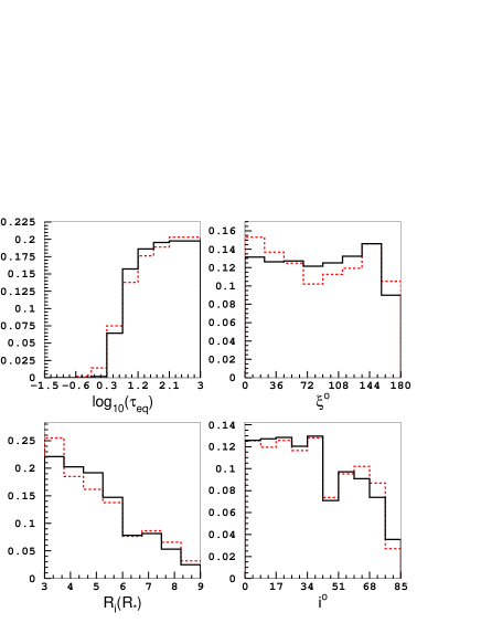
Figure 5: The photometric (black solid lines) and polarimetric (red dashed lines) efficiencies for detecting a circumstellar disk around the source star in high-magnification microlensing events versus the disk equatorial optical depth (top left panel), the angle of the lens trajectory with respect to the projected semimajor axis of disk (top right panel), the disk inner radius normalized to the source radius (bottom left panel) and the disk inclination angle (bottom right panel).

In Figure (5), we plot the photometric (black solid lines) and polarimetric (red dashed lines) efficiencies for detecting circumstellar disks around the source stars versus some relevant parameters of the disk and the source. The detection efficiency functions in terms of these parameters are given as follows.

(i) The first parameter is the disk equatorial optical depth, $\mathrm{\tau_{eq}}$. The more massive disks have higher number densities, higher equatorial optical depths and as a result the higher Stokes intensities (see the Appendix B). Hence, they have higher contributions in the total Stokes parameters (equation 15) and more chances to be detected.

(ii) The next parameter is the angle between the lens trajectory and the semimajor axis of disk, $\mathrm{\xi^{\circ}}$. The polarimetric detection efficiency maximizes when $\mathrm{\xi^{\circ}\sim 0,180}$. Because, the polarimetric time scale of disk crossing maximizes when the lens trajectory is parallel with the disk semimajor axis (see Figure 4). The photometric efficiency does not obviously depend on $\mathrm{\xi}$.

(iii) The third parameter is the disk inner radius normalized to the source radius, $\mathrm{R_{i}(R_{\star})}$. The maximum Stokes intensities due to the disk occur near the disk inner radius. The closer distance of the disk inner radius from the source center, the higher magnification factor, the larger $\mathrm{S/N}$ and as a result the higher probability for detecting disk-inducted signatures.

(iv) The last parameter is the disk inclination angle $\mathrm{i^{\circ}}$. The more inclined disks have the higher intrinsic polarization signal and the averagely shorter time scales of the disk crossing. Although, the first effect increases the polarization signals but the second decreases $\mathrm{S/N}$s. Hence, the polarimetric efficiency maximizes when $i$ is neither $\mathrm{0^{\circ}}$ nor $\mathrm{90^{\circ}}$. By more increasing the inclination angle two other effects appear which both decrease efficiencies significantly: (a) some portion of the disk located near the inner radius and above the disk semimajor axis are blocked by the source edge when $\mathrm{\varrho_{i}\cos i<\rho_{\star}}$. By increasing $i$, the larger portion of disk is blocked, whereas the blocked portions have the highest Stokes intensities. (b) The polarization of inclined disks sharply decreases by increasing the inclination angle more than $\mathrm{80^{\circ}}$ (see Figure 2).

Although the photometry and polarimetry observations of microlensing events have the same efficiencies for detecting the signature of the circumstellar disk around the source, but the polarimetry observations can give some information about the disk structure, its inner radius and its equatorial optical depth. This information can be obtained according to the position and the strength of the disk-induced polarimetric peaks in comparison with the primary peaks.

On the other hand, owing to the time interval between the primary peaks in the polarimetry curves of microlensing events and the peaks due to the disk, detecting the signatures due to disks needs doing polarimetry observations in the domains of the polarimetric curves, i.e. where the lens crosses the disk inner radius. We note that the photometric peak of disk-induced perturbations occurs at the time of the closest approach.

5 Conclusions

Gravitational microlensing is a unique method for studying the atmospheres of the Galactic bulge stars and their anomalies. One of these anomalies is the existence of a circumstellar disk around the source. In this work, we studied detecting and characterizing optically-thin disks, contain hot dusts and are located inside one Astronomical Unit from their host stars, around the Galactic bulge stars through polarimetry observations of microlensing events. Detecting these disks even around nearby stars needs high resolution observations with interferometers Absil et al. (2013). This kind of disks is the most suitable candidate to be detected with lensing. Because, the less distances from their host stars, the higher magnification factors, the higher contributions in the total Stokes parameters and higher $\mathrm{S/N}$s.

The sources surrounded by circumstellar disks have net polarization signals. Lensing can magnify these polarization signals and makes them be detected. We investigated the characteristics of the disk-induced perturbations in polarimetric microlensing events. In this regard, we summarized some significant points as follows:

(i) Disks cause that the time scale of the polarimetry curves in microlensing events increases whereas they do not change the time scale of the photometric ones. They generally break the symmetry of the polarimetry and photometry curves around the time of the closest approach.

(ii) There is a degeneracy between the geometrical parameters of the disk and its projected column density in photometric or polarimetric microlensing measurements.

(iii) If the lens moves towards the source center normal to the disk semimajor axis in some time the total polarization signal vanishes, whereas if the lens is interring the disk parallel with the disk semimajor axis, the polarization signals due to the source and disk magnify each other and the total polarization signal is always enhancing. These points help to determine the lens trajectory with respect to the disk semimajor axis.

(iv) The peaks of disk-induced perturbations in the light and polarimetry curves occur at the time of the closest approach and the time of crossing the disk inner radius respectively. According to the lens impact parameter and the disk geometrical parameters, the polarimetry curves of these microlensing events can have four, three or two nonsymmetric peaks. The time intervals between these peaks give constraints on the disk geometrical parameters and a lower limit on the disk inner radius. The ratio of these peaks also yields some information about the disk equatorial optical depth and the lens impact parameter.

Finally, We compared the efficiency for detecting disks through polarimetry observations with that through photometry observations during microlensing events by carrying out a Monte Carlo simulation. We concluded that the polarimetric and photometric efficiencies for detecting an optically-thin disk around late-type sources in high-magnification and single-lens microlensing events are similar and are about $\mathrm{38-39}$ per cent. The number of detectable optically-thin disks through these methods by monitoring $150$ million objects towards the Galactic bulge during $10$ years was estimated about $\mathrm{4}$. Noting that, the polarimetry observations help to obtain some constraints on the disk geometrical parameters specially the disk inner radius.

Acknowledgment We thank R. Ignace, J. Bjorkman and Z. Zheng and O. Absil for useful discussions and comments. We also thank the referee for valuable comments.

Appendix A Stokes intensities due to an optically-thin disk

The aim of this appendix is to describe how to calculate the Stokes intensities of a circumstellar disk. We use the formulation developed by Bjorkman & Bjorkman (1994).

To describe a star with an axisymmetric circumstellar disk, two coordinate systems are used: (a) Observer coordinate system (lens plane) $\mathrm{(x,y,z)}$ so that the projected source center is at the origin, the observer is on the $z$-axis at $\mathrm{+\infty}$ and the $\mathrm{z-y}$ plane contains the stellar rotation axis. (b) Stellar coordinate system $\mathrm{(x_{\star},y_{\star},z_{\star})}$ so that $\mathrm{z_{\star}}$ is along the stellar rotation axis and the $\mathrm{y_{\star}}$-axis is along the observer’s $x$-axis. We transform the first coordinate system to the second one by two consecutive rotations: around $z$-axis by $\mathrm{-90^{\circ}}$ and then around $y$-axis by the inclination angle $\mathrm{-i^{\circ}}$, so that:

$$x_{\star} = -y\cos i+z\sin i,$$

$$y_{\star} = x,$$

$$z_{\star} = y\sin i+z\cos i.$$ (22)

We use $\mathrm{(r,\theta,\phi)}$ to represent spherical stellar coordinate, i.e. $\mathrm{r=\sqrt{x_{\star}^{2}+y_{\star}^{2}+z_{\star}^{2}}}$, $\mathrm{\theta=\cos^{-1}(z_{\star}/r_{\star})}$, $\mathrm{\phi=\tan^{-1}(y_{\star}/x_{\star})}$ and $\mathrm{(q,\alpha,z)}$ to represent cylindrical observer coordinate, i.e. $\mathrm{q=\sqrt{x^{2}+y^{2}}}$, $\mathrm{\alpha=\tan^{-1}(y/x)}$.

The Stokes intensities $\mathrm{\boldsymbol{I}_{\nu}}$ at frequency $\nu$ are the solutions of the Stokes transfer equation which is given by Chandrasekhar (1960):

$$\frac{d}{dz}\boldsymbol{I}_{\nu}=-k_{\nu}\boldsymbol{I}_{\nu}+\boldsymbol{S}_{\nu},$$ (23)

where $\mathrm{k_{\nu}}$ is the extinction coefficient which is too small for an optically thin disk. $\mathrm{\boldsymbol{S}_{\nu}}$ is the source function which is given by:

$$\boldsymbol{S}_{\nu}=\frac{3n\sigma}{4}\left(\begin{array}[]{c}J+K_{zz}\\ K_{xx}-K_{yy}\\ -2K_{xy}\\ 0\end{array}\right),$$ (28)

where $\sigma$ is the scattering cross section and $n$ is the number density of disk (see the following section). $J$ and $\mathrm{K_{ij}}$ are the zeroth and second intensity moments respectively which are given by:

$$J = \frac{1}{4\pi}\int\boldsymbol{I}_{\nu}d\Omega,$$

$$K_{ij} = \frac{1}{4\pi}\int\boldsymbol{I}_{\nu}\hat{n}_{i}\hat{n}_{j}d\Omega,$$ (29)

where $\mathrm{\hat{n}_{i}}$ is the unit vector in the observer coordinate system, for $\mathrm{i\in(x,y,z)}$. Bjotkman and Bjorkman (1994) proposed to calculate these intensity moments in the stellar coordinate system and then using the Euler rotation matrix, $\mathrm{\boldsymbol{R}}$, obtain the intensity moments in the observer system. In that case, the convenient Euler angles are $\mathrm{(\theta,\phi,i)}$ so that $\mathrm{\boldsymbol{R}=\boldsymbol{R}_{r}(\pi/2)\boldsymbol{R}_{\phi}(i)\boldsymbol{R}_{r}(-\phi)\boldsymbol{R}_{\phi}(-\theta)}$. This matrix relates the intensity moments in the spherical polar stellar coordinate $\mathrm{(r,\theta,\phi)}$ to the cartesian observer system. Its rows 1-3 correspond to $z$, $x$ and $y$ and columns 1-3 correspond to $r$, $\mathrm{\theta}$ and $\mathrm{\phi}$. In that case the intensity moments are transformed as follows:

$$J = J^{\prime},$$

$$\boldsymbol{K} = \boldsymbol{R}\boldsymbol{K}^{\prime}\boldsymbol{R}^{T},$$ (30)

where $\mathrm{J^{\prime}}$ and $\mathrm{\boldsymbol{K}^{\prime}}$ are the related intensity moments in the spherical stellar coordinate system which are given by:

$$J^{\prime} = \frac{1}{4\pi}\int_{\Omega^{\star}}I^{\star}d\Omega^{\prime},$$

$$K^{\prime}_{ij} = \frac{1}{4\pi}\int_{\Omega^{\star}}I^{\star}\hat{n}^{\prime}_{i}\hat{n}^{\prime}_{j}d\Omega^{\prime},$$ (31)

where $\mathrm{\Omega^{\star}}$ is the solid angle subtended by the star. The unit vectors $\mathrm{\hat{n}^{\prime}_{i}}$ are given by:

$$\hat{n}^{\prime}_{r} = \cos\theta^{\prime},$$

$$\hat{n}^{\prime}_{\theta} = \sin\theta^{\prime}\cos\phi^{\prime},$$

$$\hat{n}^{\prime}_{\phi} = \sin\theta^{\prime}\sin\phi^{\prime},$$ (32)

and $\mathrm{d\Omega^{\prime}=\sin\theta^{\prime}d\theta^{\prime}d\phi^{\prime}}$. $\mathrm{I^{\star}}$ is the unpolarized stellar intensity at the stellar surface at the frequency $\mathrm{\nu}$ which has a constant amount. Indeed we assume that the disk and stellar atmosphere both are optically thin.

The emergent Stokes intensities are obtained by integrating over the source function:

$$\boldsymbol{I}(x,y)=\int_{z_{min}}^{+\infty}e^{-\tau(z)}\boldsymbol{S}_{\nu}dz$$ (33)

where $\mathrm{z_{min}}$ is the location where the line of sight intersects the stellar surface which is given by:

$$z_{min}(q)=\begin{array}[]{c}\sqrt{R_{\star}^{2}-q^{2}}~{}~{}~{}~{}~{}~{}~{}~{}(q<R_{\star})\\ -\infty~{}~{}~{}~{}~{}~{}~{}~{}~{}~{}~{}~{}~{}~{}~{}~{}~{}~{}(q\geq R_{\star})\end{array}$$ (36)

where $\mathrm{R_{\star}}$ is the source radius. The optical depth is $\mathrm{\tau(z)=\int_{z}^{+\infty}k_{\nu}~{}dz}$. Note that we separately calculate the contribution of the source Stokes intensities which is due to the stellar atmosphere (see equation 15).

Appendix B Disk density

We use the following model for the number density in the disk Christopher et al. (1996):

$$n(R,z)=n_{0}(\frac{R_{c}}{R})^{\gamma}\exp[-\frac{z^{2}}{2H(R)^{2}}],$$ (37)

where $\mathrm{R_{c}}$ is the length scale, $\mathrm{\gamma}$ specifies the radial dependence of the disk surface density and $\mathrm{H(R)=h_{0}(\frac{R}{R_{s}})^{\beta}}$ is the disk thickness at the redial distance of $R$ from the disk center. $\mathrm{h_{0}}$ is the hight scale at the radial distance $\mathrm{R_{s}}$. $\mathrm{n_{0}}$ is the number density in the mid-plane and at the radial distance $\mathrm{R_{c}}$ which is a function of the disk mass $\mathrm{M_{d}}$ Williams & Cieza (2011):

$$n_{0}=\frac{(2-\gamma+\beta)}{(2\pi)^{3/2}h_{0}R^{2}_{i}m_{0}}(\frac{R_{s}}{R_{i}})^{\beta}M_{d},$$ (38)

where $\mathrm{m_{0}\simeq 2.3m_{p}}$ is the mean molecular weight and $\mathrm{m_{p}}$ is the proton mass Dullemond & Monnier (2010). For this disk density, the equatorial optical depth is given by:

$$\tau_{eq}=\int_{R_{i}}^{\infty}dRn(R,0)\sigma=n_{0}\sigma R_{i}(\frac{R_{c}}{R_{i}})^{\gamma}/(\gamma-1).$$ (39)

Throughout the paper, we set $\mathrm{R_{c}=R_{i}}$. Hence the disk equatorial optical depth is $\mathrm{\tau_{eq}=n_{0}\sigma R_{i}/(\gamma-1)}$. The source function, given by equation (28), is proportional to $\mathrm{\tau_{eq}(\gamma-1)/R_{i}}$. Therefore, the disk Stokes intensities and as a result the disk polarization signal are proportional to the disk equatorial optical depth.

References

- Absil et al. (2013) Absil O., Defrére D., Coudé du Foresto V., 2013, AAP, 555, L104.
- Agol (1996) Agol E., 1996, MNRAS, 279, L571.
- Bjorkman & Bjorkman (1994) Bjorkman J. E., Bjorkman K. S., 1994, ApJ, 436, L818.
- Bogdanov et al. (1996) Bogdanov M. B., Cherepashchuk A. M., Sazhin M. V., 1996, Ap & SS, 235, L219.
- Bozza & Mancini (2002) Bozza V., Mancini L., 2002, A & A, 394, L47.
- Chandrasekhar (1960) Chandrasekhar S., 1960, Radiative Transfer. Dover Publications, New York.
- Christopher et al. (1996) Christopher J., et al., 1996, ApJ, 473, L437.
- Dullemond & Monnier (2010) Dullemond C. P., Monnier J. D., 2010, A. R. A& A, 48, L205.
- Einstein (1936) Einstein A., 1936, Science, 84, L506.
- Ertel et al. (2014) Ertel S., Absil O., Defrére D., et al., 2014, A & A, 570, L128.
- Fluri & Stenflo (1999) Fluri D.M., Stenflo J. O., 1999, A & A, 341, L902.
- Gaudi (2012) Gaudi B.s., 2012, A. R. A& A, 50, L411.
- Halonen et al. (2013) Halonen R. J., Mackay F. E., Jones C. E., 2013, ApJS, 204, L11.
- Halonen & Jones (2013) Halonen R. J., Jones C.E. 2013, ApJ, 765, L17.
- Høg et al. (1995) Høg E., Novikov I. D., Polnarev, A. G. 1995, A & A , 294, L287.
- Hundertmark et al. (2009) Hundertmark M., Hessman F.V., Dreizler S., 2009, A & A, 500, L929.
- Ignace et al. (2006) Ignace R., Bjorkman J. E., Bryce H. M., 2006, MNRAS, 366, L92.
- Ingrosso et al. (2012) Ingrosso G., Calchi Novati S., De Paolis F., et al. 2012, MNRAS, 426, L1496.
- Ingrosso et al. (2015) Ingrosso G., Calchi Novati S., De Paolis F., et al. 2015, MNRAS, 446, L1090.
- Kains et al. (2013) Kains N., Street R., Choi J-Y., et al., 2013, A & A, 552, L70.
- Lamers & Cassinelli (1999) Lamers H.J., Cassinelli J.P., 1999, Introduction to Stellar Winds. Cambridge Univ. Press, Cambridge
- Mao (2012) Mao S., 2012, Research in A & A, 12, 1.
- Miralda-Escdé (1996) Miralda-Escudé J., 1996, ApJ, 470, L113.
- Paczyński (1986) Paczyński, B. 1986, ApJ, 304, 1.
- Paczyński (1997) Paczyński B., 1997, Astrophys. J. Lett. astro-ph/9708155.
- Rahvar et al. (2003) Rahvar S., Moniez M., Ansari R., Perdereau, O., 2003, A& A, 412, L81.
- Rahvar (2015) Rahvar, S., 2015, IJMPD, 24, 1530020(arXiv:1503.04271v1).
- Sajadian (2014) Sajadian S., 2014, MNRAS, 439, L3007.
- (29) Sajadian S., 2015a, AJ, 149, L147.
- (30) Sajadian S., 2015b, MNRAS, 452, L2587.
- Sajadian & Rahvar (2012) Sajadian S., Rahvar S., 2012, MNRAS, 419, L124.
- Sajadian & Rahvar (2015) Sajadian S., Rahvar S., 2015, MNRAS, 452, L2579.
- Schemid et al. (2002) Schemid, Appenzeller, Stenflo & Kaufer, 2002, Proceedings of the ESO Workshop, Germany, (ESO,2002), L231.
- Schneider & Wagoner (1987) Schneider P., Wagoner R. V., 1987, ApJ, 314, L154.
- (35) Simmons J. F. L., Newsam A. M., Willis J. P., 1995a, MNRAS, 276, L182.
- (36) Simmons J. F. L., Willis J. P., Newsam A. M., 1995b, A & A, 293, L46.
- Simmons et al. (2002) Simmons J.F.L., Bjorkman J.E., Ignace R., Coleman I.J., 2002, MNRAS, 336, 501.
- Stenflo (2005) Stenflo J.O., 2005, A & A, 429, L713.
- Sumi et al. (2006) Sumi T., et al. 2006, ApJ 636, L240.
- Tinbergen (1996) Tinbergen J., 1996, Astronomical Polarimetry. Cambridge Univ. Press, New York.
- Walker (1995) Walker M.A. 1995, ApJ, 453, L37.
- Williams & Cieza (2011) Williams J.P., Cieza L.A., 2011, arXiv:1103.0556.
- Wyrzykowski et al. (2014) Wyrzykowski, Ł., et al., 2014, arXiv:1405.3134.
- Yoshida (2006) Yoshida H., 2006, MNRAS, 369, L997.
- Zheng & Ménard (2005) Zheng Z., Ménard B., 2005, ApJ, 635, L599.