The role of the diffusive protons in the $\gamma$-ray emission of supernova remnant RX J1713.7$-$3946 — a two-zone model

Abstract

RX J1713.7$-$3946 is a prototype in the $\gamma$-ray-bright supernova remnants (SNRs) and is in continuing debates on its hadronic versus leptonic origin of the $\gamma$-ray emission. We explore the role played by the diffusive relativistic protons that escape from the SNR shock wave in the $\gamma$-ray emission, apart from the high-energy particles’ emission from the inside of the SNR. In the scenario that the SNR shock propagates in a clumpy molecular cavity, we consider that the $\gamma$-ray emission from the inside of the SNR may arise either from the inverse Compton scattering or from the interaction between the trapped energetic protons and the shocked clumps. The dominant origin between them depends on the electron-to-proton number ratio. The diffusive protons that escaped from the shock wave during the expansion history can provide an outer hadronic $\gamma$-ray component by bombarding the surrounding dense matter. The broadband spectrum can be well explained by this two-zone model, in which the $\gamma$-ray emission from the inside governs the TeV band, while the outer emission component substantially contributes to the GeV $\gamma$-rays. The two-zone model can also explain the TeV $\gamma$-ray radial brightness profile that significantly stretches beyond the nonthermal X-ray-emitting region. In the calculation, we present a simplified algorithm for Li & Chen’s (2010) “accumulative diffusion” model for escaping protons and apply the Markov Chain Monte Carlo method to constrain the physical parameters.

1 INTRODUCTION

It is usually believed that Galactic supernova remnants (SNRs) are the main accelerators of cosmic rays (CRs, mainly protons) and can boost particles up to the “knee” energy of $\sim$3 $\times\ 10^{15}$ eV through the diffusive shock acceleration (DSA). An important probe of this conjecture is the hadronic $\gamma$-ray emission (namely, $\pi^{0}$-decay $\gamma$-rays produced in the inelastic collision between the accelerated protons and the target baryons) from the SNRs that interact with molecular clouds (MCs). Fortunately, great progress has been made in understanding the SNR paradigm by the detection of a characteristic $\pi^{0}$-decay “bump” in the interacting SNRs IC 443 (Ackermann et al., 2013) and W44 (Giuliani et al., 2011; Ackermann et al., 2013; Cardillo et al., 2014). Yet, multifaceted investigations of hadronic interaction are still needed to increase and strengthen the evidence for the paradigm in a large sample of SNR-MC association systems (e.g., Jiang et al., 2010). It is, however, often uneasy to distinguish the nature of the $\gamma$-rays between the hadronic scenario and leptonic (inverse Compton [IC] and/or bremsstrahlung) scenario even in the SNR-MC systems, such as SNR RX J1713.7$-$3946, and deep explorations for the spectral properties and emitting mechanism of them in the GeV–TeV range are essential.

SNR RX J1713.7$-$3946 (G347.3$-$0.5) was discovered by ROSAT X-ray observations (Pfeffermann & Aschenbach, 1996, pp. 267-68) and suggested to be the remnant of the historical supernova AD 393 (Wang et al. 1997; hereafter an age of the remnant $t_{\rm age}\sim 1620$ yr will be used). Its shell-like X-ray emission is dominated by a nonthermal component and a lack of thermal line features (e.g., Koyama et al., 1997; Slane et al., 1999; Cassam-Chenaï et al., 2004). It is found to be confined in a molecular cavity, and the elevated gas temperature and broad molecular line wings in a few molecular cloudlets are ascribed to the high-energy events of the SNR (Fukui et al., 2003; Moriguchi et al., 2005). The molecular cavity can be reasonably understood as the product of the energetic stellar wind and ionizing photons of the massive progenitor star (which is suggested to be no later than B0–B1 type, with a mass $\gtrsim$15 $\pm\ 2\ M_{\odot}$; Chen et al. 2013). In the radio band, it shows faint emission and has an average angular diameter of $60^{\prime}$, corresponding to an average radius $R_{s}\,\sim\,9$ pc at distance $d\,\approx\,1$ kpc (e.g. Fukui et al., 2003; Moriguchi et al., 2005). It is suggested that the SNR is in the free expansion evolutionary phase (e.g. Moriguchi et al., 2005; Sano et al., 2010) and that the forward shock has not yet reached the wall enclosing the wind-blown cavity in view of the high velocity currently measured (Federici et al., 2015).

Since the detection of TeV $\gamma$-ray emission from it (Enomoto et al., 2002; Aharonian et al., 2004, 2007), SNR RX J1713.7$-$3946 has garnered an enormous amount of attention and aroused constant debates on the hadronic versus leptonic origin of its $\gamma$-ray emission (e.g. Aharonian et al., 2006; Berezhko & Völk, 2008; Liu et al., 2008; Morlino et al., 2009; Zirakashvili & Aharonian, 2010). The debates seemed to have been concluded when the 2 yr Fermi-LAT observations revealed a hard GeV spectrum with a power-law photon index $\Gamma=1.5\pm 0.1$ (Abdo et al., 2011), which appears to support the leptonic scenario (e.g., Abdo et al., 2011; Li et al., 2011; Yuan et al., 2011; Ellison et al., 2012; Finke & Dermer, 2012; Lee et al., 2012). Subsequently, however, a strong correlation of azimuthal distribution was found between the TeV $\gamma$-ray flux and the column density of total interstellar protons, which is in favor of a hadronic origin of the $\gamma$-rays (Fukui et al., 2012). Some hadronic interaction models have also been elaborated to interpret the hard GeV emission (Inoue et al., 2012; Gabici & Aharonian, 2014; Federici et al., 2015).

Both scenarios in terms of relativistic leptons and protons accelerated via standard DSA can explain the hard spectrum with their advantages, but meanwhile also present difficulties. In the context of pure leptonic processes, the IC scattering seems to naturally explain the hard GeV $\gamma$-ray spectrum without any extra assumptions and can be well compatible with the lack of thermal X-ray line emission. A leptonic origin of the TeV emission is strongly suggested by Li et al. (2011) using a spectral inversion method independent of the particle acceleration model. The morphology in TeV band closely matches the nonthermal shell in the radio and X-ray bands (Aharonian et al., 2006), also suggesting an origin from the same electron population. On the other hand, it is pointed out that single-zone distribution of elections encounters a difficulty in providing a good fit to its broadband spectral energy distribution (SED; Finke & Dermer, 2012). Also, if the $\gamma$-ray emission is leptonic dominated, it remains perplexity why it does not contain any significant hadronic contribution, given the observational fact that the SNR is environed by molecular gas.

In the context of pure hadronic processes, an inhomogeneous shocked medium with dense clumps (Inoue et al., 2012; Gabici & Aharonian, 2014) and a dense shell outside the SNR without contact (Federici et al., 2015) are invoked. In the former case, Inoue et al. (2012) consider that, in the downstream of the shock wave, the penetration depth regulated by energy dependence of Bohm diffusion is generally shorter than the thickness of clumps, which gives the mass of the proton-illuminated gas depending on the energy of incident protons $M(E_{\rm p})\propto E_{\rm p}^{1/2}$ and hence a $\gamma$-ray index 0.5 smaller than that of the parent protons. Alternatively, Gabici & Aharonian (2014) suggest that, because of turbulent layers surrounding the clumps, only protons above a minimum energy can effectively diffuse into clumps, which may result in a hard proton spectrum below that energy in clumps. It is, however, difficult in this case to explain why no thermal X-ray line emission from the shocked dense medium is observed. Possibly, the dense clumps swept up by the shock wave can survive and still remain a temperature too low to produce thermal X-rays (Inoue et al., 2012; Gabici & Aharonian, 2014). In the latter case, the dense shell (within a thickness of $\sim$0.3 pc) outside the SNR is effectively illuminated by TeV protons in the CR precursor region, giving rise to a hard $\gamma$-ray spectrum (Federici et al., 2015). In this case, the shock does not interact with dense material, and thus the difficulty with the lack of thermal X-rays can be avoided (although the model fluxes in $\sim$10 GeV–1 TeV appear to be underestimated).

Here we explore the role played by the diffusive relativistic protons that escape from the SNR shock wave and hit the surrounding dense gas in the $\gamma$-ray emission of RX J1713.7$-$3946, considering that the blast wave is propagating in a molecular cavity, in which there may be a mount of shocked clumps. Most recently, the TeV $\gamma$-ray emission has been found to stretch noticeably beyond the nonthermal X-ray emission region, also indicating a contribution of the escaping protons to the $\gamma$-ray emission (de Naurois, 2015, and references therein). Currently, there are two types of mechanisms in essence suggested for hadronic emission: $\pi^{0}$ decay not only can take place in shock-crushed dense clouds (e.g., Blandford & Cowie, 1982; Uchiyama et al., 2010; Tang & Chevalier, 2014) but also can occur in the adjacent MCs illuminated by diffusive escaping protons (e.g., Aharonian & Atoyan, 1996; Gabici et al., 2009; Li & Chen, 2010; Ohira et al., 2011). In the following, we show that the GeV–TeV $\gamma$-ray spectrum of RX J1713.7$-$3946 with updated 5 yr Fermi-LAT data can be perfectly interpreted with a two-zone scenario, in which the $\pi^{0}$-decay $\gamma$-rays resulting from the diffusive protons will substantially contribute to the GeV $\gamma$-rays while the leptonic process or the $p$–$p$ interaction in the shocked clumps will be responsible for the TeV $\gamma$-rays. In the calculation, we present a simplified algorithm for the “accumulative diffusion” model for escaping protons developed by Li & Chen (2010) and apply the Markov Chain Monte Carlo (MCMC) method to constrain the model parameters.

2 A TWO-ZONE MODEL

Here we consider two $\gamma$-ray-emitting zones for SNR RX J1713.6$-$3946. The first zone is the cavity wall (the dense matter at the cavity boundary), which is bombarded by the protons that escaped from the shock wave during the history of expansion. The second zone is inside the SNR, and the emission could be either IC scattering off the accelerated electrons (Model Ia) or the hadronic emission from the shocked clumps (Model IIa).

It is suggested that CR protons that escape from SNRs can illuminate the nearby massive clouds and produce $\gamma$-rays (Aharonian & Atoyan, 1996). Some possible evidence for this scenario has been obtained by the observation of diffuse $\gamma$-ray emission from the vicinity of SNR shells, such as in W44 (Uchiyama et al., 2012), with which massive MCs are spatially coincident. The model has successively been improved and applied to a number of SNR-MC systems to explain the origin of the $\gamma$-ray emission (e.g., Gabici et al., 2009; Li & Chen, 2010, 2012; Ohira et al., 2011; Nava & Gabici, 2013). In the case of RX J1713.7$-$3946, although the blast wave may not have hit upon the cavity wall (e.g. Inoue et al., 2012), a considerable fraction of the escaping protons have arrived at the wall. It can be expected that the $p$–$p$ collision between these protons with the molecules in the wall gives birth to $\pi^{0}$ decay $\gamma$-rays. This emission, together with the leptonic emission from the electrons and/or the hadronic emission from the shocked clumps, will be calculated below to jointly interpret the spectral and spatial behavior of the $\gamma$-rays from the SNR.

2.1 Simplified Algorithm for the Accumulative Diffusion Model

For the continuous injection of the accelerated protons that escape from the propagating shock wave surface, Li & Chen (2010) established an “accumulative diffusion” model, in which the protons at a given position are a collection of the diffusive protons escaping from the entire shock surface at different radii throughout the history of the SNR expansion. They derived the proton distribution by integrating the solution of the diffusion equation given by Aharonian & Atoyan (1996) for the impulsive point-like source injection (see Equations. (1)–(2) in Li & Chen, 2010). Actually, the algorithm of the model can be simplified by directly solving the diffusion equation of the escaping protons as follows.

Ignoring protons’ energy losses, the diffusion equation in the spherically symmetric case is written as

$$\frac{\partial}{\partial t}f(E_{\rm p},R,t)=\frac{D(E_{\rm p})}{R^{2}}\frac{\partial}{\partial R}R^{2}\frac{\partial}{\partial R}f(E_{\rm p},R,t)+Q(E_{\rm p},R,t),$$ (1)

where $f(E_{\rm p},R,t)$ is the distribution of the escaping protons with energy $E_{\rm p}$ at a given distance $R$ from the SNR center at a given time $t$ from the explosion time, $Q(E_{\rm p},R,t)$ is the source injection function, and $D(E_{\rm p})$ is the diffusion coefficient. Here we assume that the diffusion coefficient has the form of $D(E_{\rm p})=10^{28}\chi(E_{\rm p}/10\,{\rm GeV})^{\delta}\ {\rm cm^{2}}\,{\rm s^{-1}}$, where $\chi$ is the correction factor of slow diffusion around the SNR and $\delta\approx 0.3$–0.7 (Berezinskii et al., 1990) is the index of diffusion coefficient. Following the treatment in Atoyan et al. (1995), we define a new function $F(E_{\rm p},R,t)=Rf(E_{\rm p},R,t)$, and then Equation (1) reads as

$$\frac{\partial}{\partial t}F(E_{\rm p},R,t)=D(E_{\rm p})\frac{\partial^{2}}{\partial R^{2}}F(E_{\rm p},R,t)+Q(E_{\rm p},R,t)\,R.$$ (2)

The Green function for Eq. (2), namely, the solution for point-like impulsive injection source $Q(E_{\rm p},R,t)R=\delta(R-\xi)\delta(t-t_{i})$, is (Atoyan et al., 1995)

$$G(E_{\rm p},R,t;\xi,t_{i})=\frac{1}{\sqrt{\pi}R_{\rm d}}\left\{\exp\left[-\left(\frac{R-\xi}{R_{\rm d}}\right)^{2}\right]-\exp\left[-\left(\frac{R+\xi}{R_{\rm d}}\right)^{2}\right]\right\},$$ (3)

where $R_{\rm d}=2\sqrt{D(t-t_{i})}$ is the diffusion radius.

The injection function of the protons that escape from the shock front is

$$Q(E_{\rm p},R,t)=\frac{Q_{\rm p}(E_{\rm p})}{4\pi R^{2}}\delta(R-R_{s}(t)),$$ (4)

where $Q_{\rm p}(E_{\rm p})$ is the injection rate from the spherical surface $4\pi R^{2}$ and $R_{s}(t)$ is the shock radius. The solution of Equation (1) is

$$\begin{split}f(E_{\rm p},R,t)=&\frac{1}{R}\int^{t}_{0}\int^{\infty}_{0}Q(E_{\rm p},\xi,t_{i})\xi G(E_{\rm p},R,t;\xi,t_{i}){\rm d}\xi{\rm d}t_{i}\\ =&\int^{t}_{0}\frac{Q_{\rm p}(E_{\rm p})}{4\pi^{3/2}R_{s}(t_{i})R_{\rm d}R}\left\{\exp\left[-\left(\frac{R-R_{s}(t_{i})}{R_{\rm d}}\right)^{2}\right]-\exp\left[-\left(\frac{R+R_{s}(t_{i})}{R_{\rm d}}\right)^{2}\right]\right\}{\rm d}t_{i}.\end{split}$$ (5)

This solution, with a single integral, is equivalent to Equation (2) in Li & Chen (2010), which is a triple integral, and will be reduced to Equation (8) in Aharonian & Atoyan (1996) for the case of point-like continuous injection as $R_{s}\rightarrow 0$.

2.2 Model Fit to the Broadband SED

The shock-accelerated particles are assumed to obey a power-law distribution with a high-energy cutoff:

$$dN_{i}/dE_{i}=A_{i}E_{i}^{-\alpha_{i}}\times\exp(-E_{i}/E_{{\rm c},i})$$ (6)

where $i={\rm e,p}$, $E_{i}$ is the particle kinetic energy, $\alpha_{i}$ is the power-law spectral index and is taken as $\alpha_{\rm e}=\alpha_{\rm p}=\alpha$, and $E_{{\rm c},i}$ is the cutoff energy and will be set to the CR “knee” energy for the protons, leaving $E_{\rm c,e}$ as a free parameter. The normalization parameter $A_{i}$ is determined from the total kinetic energy of particles above 1 GeV.

In our calculation, two physical parameters are adopted instead of the normalization parameters: the energy conversion efficiency $\eta$, namely, the faction of explosion energy converted to CR energy, and the number ratio between the accelerated electrons and protons at 1 GeV, $K_{\rm ep}=A_{\rm e}/A_{\rm p}$. The energy conversion efficiency ($\eta$) is always difficult to determine directly from the acceleration theory, and there is usually not a consensus in the value of the energy conversion efficiency. In the cr-hydro-NEI modeling for SNR RX J1713.7$-$3946, it was suggested that about 16% of the explosion energy has converted into the accelerated particles (Lee et al., 2012). A lower value of 6% was obtained via modeling the $\gamma$-ray emission (Gabici & Aharonian, 2014). For electron-to-proton number ratio ($K_{\rm ep}$), an order of 0.01 was derived from the CRs measured at Earth and a lower limit, $\gtrsim$$10^{-3}$, was implied according to the radio observations of the SNRs in nearby galaxies (Katz & Waxman, 2008).

The distribution of the escaping protons, $f(E_{\rm p},R_{w},t_{\rm age})$, is obtained from Equation (5), where $R_{w}$ is the radius of the cavity wall and is set to be $\sim$10 pc. In the calculation, following Cassam-Chenaï et al. (2004), we assume that the SNR radius conforms to the self-similar solution for the free expansion phase (Chevalier, 1982), $R_{s}(t)\propto t^{(n-3)/(n-s)}$, where $n$ and $s$ are the power-law indices of the initial outer density profile in the ejecta and of the initial ambient medium density profile. Here we take $n=9$ and $s=0$ (for a shocked wind-dominated medium), but taking $n=12$ or $s=2$ will produce a similar result in our calculation. We adopt the average remnant radius $R_{s}\approx 9$ pc at present time $t_{\rm age}=1620$ yr. The injection rate is given by $5t_{\rm age}Q_{\rm p}(E_{\rm p})=dN_{\rm p}/dE_{\rm p}$. Based on the calculations of (Lee et al., 2012), we assume that about 20% of the accelerated protons escape from the SNR. The explosion energy of the SNR is assumed to be $10^{51}$ erg.

For the hadronic $\gamma$-ray emission, we use the analytic photon emissivity developed by Kelner et al. (2006) for $p$–$p$ interaction, including the enhancement factor of 1.84 due to the contribution from heavy nuclei (Mori, 2009). We calculate the leptonic emission following Blumenthal & Gould (1970). In addition to the cosmic microwave background, the seed photons also include the Galactic interstellar infrared photons at 30 K with an energy density of 0.3 eV cm^-3 (Porter et al., 2006).

Two cases will be considered for the $\gamma$-ray emission arising from the inside of the SNR: (I) it is dominated by the IC process of the accelerated electron; and (II) it is dominated by the collision of the accelerated protons with the shocked clumps.

2.2.1 Case I: Leptonic Emission Dominated Inside

On the inner side of the shock front, the $\gamma$-ray emission is assumed to be mainly from the shock-accelerated electrons, which are also producing the synchrotron emission in the spectral range from radio to X-rays. The leptonic process in this SNR has often been considered as the origin of the $\gamma$-ray emission from it, chiefly owing to the consistency with the hard GeV $\gamma$-ray spectrum, the lack of thermal X-ray emission, and its location in a low-density cavity of molecular gas. In this case, we adopt a typical electron-to-proton number ratio $K_{\rm ep}$ = 0.01. (With this parameter, the $\gamma$-ray emission from the possibly shocked clumps will be insignificant, as can be seen in the following results.)

There are seven parameters in this case (for the combined contribution from the outside diffusive protons and inside electrons; Model Ia): $\eta$, $\alpha$, $\delta$, $\chi$, $E_{\rm c,e}$, $B_{\rm SNR}$, and $M_{\rm t}$, where $B_{\rm SNR}$ is the average magnetic field at the shock and $M_{\rm t}$ is the mass of the baryon targets in the cavity wall bombarded by the escaping protons. To constrain the model parameters, we employ the MCMC approach, which, based on the Bayesian statistics, is better than the grid approach, with a more efficient sampling of the parameter space of interest, especially for high dimensions. A brief introduction to the basic procedure of the MCMC sampling can be found in Fan et al. (2010), and more details can be found in Neal (1993), Gamerman (1997), and Mackay (2003). In our MCMC fitting calculation, all parameters are set to be free, but $\delta$ is confined in the range 0.3–0.7, and the observational data with only upper limits are excluded.

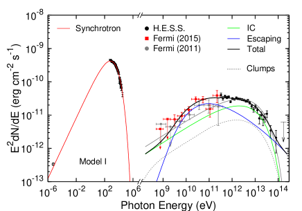
Figure 1: Fitted results for Model Ia. Left: 1D probability distribution of the parameters; Right: best-fitted broadband SED of SNR RX J1713.7$-$3946 according to the radio (Acero et al., 2009), X-ray (Tanaka et al., 2008), GeV (Fermi: Abdo et al. 2011, Federici et al. 2015), and TeV (HESS: Aharonian et al. 2011) data. The gray solid line represents the fitting SED for Model Ib.

The one-dimensional (1D) probability distributions of model parameters and the best-fit SED are shown in Figure 1. The 1D probability distribution of each parameter converges well with a single peak (left panel of Figure 1). The best-fit parameters with 1$\sigma$ statistical uncertainties and the $\chi^{2}$ values are listed in Tables 1 and Table 2, respectively. The model $\gamma$-ray SED (see right panel of Figure 1) shows that this model perfectly explains the $\gamma$-ray data. In the energy range $\sim$3–500 GeV, the $\gamma$-rays are mainly contributed by the hadronic emission with a peak flux therein; in the remaining regime, they are dominated by the leptonic emission. The fluxes above 0.25 TeV of the hadronic (outer) and leptonic (inner) components are about $5.3\times 10^{-11}\,{\rm erg\,cm^{-2}\,s^{-1}}$ and $7.6\times 10^{-11}\,{\rm erg\,cm^{-2}\,s^{-1}}$, respectively. The fluxes in the range from 0.3 to 40 TeV of the outer and inner components are about $4.7\times 10^{-11}\,{\rm erg\,cm^{-2}\,s^{-1}}$ and $7.3\times 10^{-11}\,{\rm erg\,cm^{-2}\,s^{-1}}$, respectively. For the escape process, we got $\chi\sim 0.01$, which is similar to the previous estimates for SNR environs (e.g., Fujita et al., 2010; Li & Chen, 2012; Ohira et al., 2012; Tang & Chevalier, 2015), and $\delta\sim 0.65$, which is in the normal range. The mass of the baryon targets, $8.8\times 10^{3}M_{\odot}$, seems reasonable as compared to the estimate of the surrounding interstellar protons reservoir, $2\times 10^{4}M_{\odot}$ (Fukui et al., 2012). In addition, the $\gamma$-ray emission from the possibly shocked clumps (see the next subsection for description) in this case is also plotted by gray dotted line in Figure 1, implying an insignificant contribution to the total $\gamma$-ray emission.

For comparison, we also test the notion of the pure leptonic process as the origin of the GeV–TeV $\gamma$-rays, incorporating the updated Fermi data (Model Ib). The best-fit SEDs are displayed by the gray solid line in Figure 1. The model parameters and $\chi^{2}$ values of the best fit are also listed in Tables 1 and 2, respectively. The $\chi^{2}$ values in various wavebands are obviously higher than those in Model Ia except in the radio. The best-fit SED shows that the pure leptonic model underestimates the GeV flux, similar to the results of previous multiband fits with simple leptonic models (e.g., Fan et al., 2010; Finke & Dermer, 2012). In addition, we also calculate the $\chi^{2}$ value in the GeV band using our best-fit SED and the previous Fermi data (Abdo et al., 2011), which are listed in Table 2 in parentheses.

2.2.2 Case II: Hadronic Emission Dominated Inside

In this case, the $\gamma$-ray emission in the downstream are mainly from the decay of the neutral pions generated in the inelastic collision between the relativistic protons and shocked dense clumps. It is pointed out that there may be some dense clumps shocked by the blast wave, which can act as a target for the bombardment of energetic protons (e.g. Moriguchi et al., 2005; Sano et al., 2010, 2013). As mentioned in section Section 1, a few hadronic models have been proposed to interpret the observed GeV–TeV $\gamma$-ray spectrum. The IC $\gamma$-ray generation may be suppressed owing to the high magnetic field amplified by the turbulence induced by the shock–cloud interaction (e.g. Inoue et al., 2012). This case requires a relatively small amount of electrons (for the synchrotron), and thus we adopt a low value of the electron-to-proton number ratio, $K_{\rm ep}=10^{-3}$.

Following Inoue et al. (2012), the total mass of the gas in the clumps directly bombarded by the accelerated protons, $m_{\rm c,tot}$, can be obtained via three steps: (1) Estimate the average mass density $\rho_{\rm c}$ for each clump with physical parameters given by Sano et al. (2013, see their Tables 3 and 4). (2) Estimate the mass in the outer layer of each clump that is penetrated by relativistic protons using $m_{\rm c}=4\pi\rho_{\rm c}a_{\rm c}^{2}\,l_{\rm pd}$ (see Inoue et al., 2012), where $a_{\rm c}$ is the clump radius and $l_{\rm pd}$ is the penetration depth of the accelerated protons into the clumps during diffusion time $t_{\rm pd}$. The diffusion time is estimated as $t_{\rm pd}\sim 0.2\,(l_{m}/1\,{\rm pc})(V_{s}/4000\,{\rm km\,s^{-1}})^{-1}\,{\rm kyr}$, where $V_{s}=4000\,{\rm km\,s^{-1}}$ (e.g., Cassam-Chenaï et al., 2004; Acero et al., 2009) is the shock velocity and $l_{m}\sim$ 1 pc is the mean length that the shock moves forward from the clumps, estimated from the spatial distribution of the clumps (Sano et al. 2013). (3) Scale the mass of the gas collided by protons according to the area fraction covered by X-rays for each clump and sum the mass of the clumps. Hence, we obtain

$$m_{\rm c,tot}\approx 13\,\left(\frac{\eta_{\rm B}}{1}\right)\left(\frac{E_{\rm p}}{10\,{\rm GeV}}\right)^{1/2}\left(\frac{B_{\rm MC}}{100\,\mu{\rm G}}\right)^{-1/2}\left(\frac{t_{\rm pd}}{0.2\,{\rm kyr}}\right)^{1/2}M_{\odot},$$ (7)

where $\eta_{\rm B}$ is the degree of magnetic field fluctuations and $B_{\rm MC}$ is the magnetic field in the dense region of MCs (see Inoue et al., 2012). We assume that the trapped accelerated protons which uniformly distribute in the downstream have a power-law energy distribution, which can also be described by Equation (6). In order to account for the HESS data, however, the proton cutoff energy needs to be a free parameter to be decided.

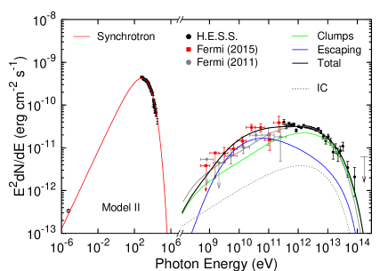
Figure 2: Same as in Figure 1 but for Model IIa. The gray solid line in the right panel represents the fitting SED for Model IIb.

There are eight parameters for the combined contribution from the outside diffusive protons and inside trapped protons (Model IIa): $\eta$, $\chi$, $\alpha$, $\delta$, $B_{\rm SNR}$, $E_{\rm c,e}$, $E_{\rm c,p}$, and $M_{\rm t}$, which are constrained by using the MCMC method. The 1D probability distributions of model parameters and the best-fit SED are shown in Figure 2. The best-fit parameters with 1$\sigma$ statistical uncertainties and the $\chi^{2}$ values are also listed in Tables 1 and 2, respectively. Similar to that in Model Ia, the model $\gamma$-ray SED (see right panel in Figure 2) also is the sum of two components, the $\gamma$-ray emission from the shocked clumps penetrated by the trapped protons and the cavity wall illuminated by the escaping protons. In the energy range $\sim$2–200 GeV, the $\gamma$-rays are mainly contributed by the escaping protons with a peak flux therein; in the remaining range, they are dominated by the contribution of the trapped protons. The fluxes above 0.25 TeV from the escaping (outer) and trapped (inner) protons are about $3.4\times 10^{-11}\,{\rm erg\,cm^{-2}\,s^{-1}}$ and $8.7\times 10^{-11}\,{\rm erg\,cm^{-2}\,s^{-1}}$, respectively. The 0.3–40 TeV fluxes for the outer and inner components are about $3.1\times 10^{-11}\,{\rm erg\,cm^{-2}\,s^{-1}}$ and $8.4\times 10^{-11}\,{\rm erg\,cm^{-2}\,s^{-1}}$, respectively. Parameters $\chi$ and $\delta$ (for the escaping protons) are similar to those in Model Ia. The IC $\gamma$-ray emission is trivial in this case, as displayed with gray dotted line in Figure 2.

We also consider the downstream proton–clump interaction as the only mechanism of the GeV–TeV $\gamma$-ray emission (referred to Model IIb), with the spectral fit parameters also listed in Tables 1 and 2. The best-fit SED is displayed by the gray solid line in Figure 2 and shows that the contribution from the interaction between the trapped protons and the shocked clumps alone will also underestimate the GeV flux.

3 DISCUSSION

As stated above, although the pure IC scattering or the pure shock–clump interaction inside the SNR can explain the low spectral index at GeV band, such simple models tend to underestimate the GeV-band flux. In view of the expansion of the SNR in a molecular cavity and the presence of the dense molecular gas surrounding the SNR, we additionally take into account the role of the energetic protons that escaped from the blast shock during the expansion history. These protons can contribute the $\gamma$-ray emission due to “illumination” of the nearby dense gas due to $p$–$p$ collision. Considering that the SNR shock is still propagating in the low-density medium (in which there may be interspersal dense clumps), we have calculated this illumination effect on the broadband spectrum of SNR RX J1713.7$-$3946 in a two-zone model.

3.1 Spectral Behavior of the Gamma-ray Emission

From the fitted SED and the $\chi^{2}$ value, we can see that both Model Ia and Model IIa give similarly good results and the hadronic $\gamma$-ray emission from the escaping protons plays an important role in the explanation of the spectral data, especially in the GeV band. The flux of this component, peaking around $\sim 80$ GeV, naturally compensates the underestimate at the GeV band in the aforementioned simple models. From the point of view of spectral shape, the hadronic spectrum from the inside clumps (in Model IIa) actually has a similar effect on the total $\gamma$-ray emission to the leptonic one (in Model Ia). Given the presence of the shocked clumps, the dominant mechanism of $\gamma$-ray emission in the downstream depends on the electron-to-proton number ratio, $K_{\rm ep}$: it was found that the hadronic emission from the inside clumps dominates for $K_{\rm ep}$ $<\,\sim$4$\times 10^{-3}$ while the leptonic component dominates for $K_{\rm ep}$ $>\,\sim$4$\times 10^{-3}$. Both models give a small energy transfer fraction $\eta<10\%$ for this young SNR, similar to those suggested for SNRs Cas A (e.g. Abdo et al., 2010) and Tycho (e.g. Zhang et al., 2013).

The two models entail different cutoff energies $E_{\rm c,p}$ of shock-accelerated protons. It is constrained as $81^{+14}_{-12}$ TeV by the current HESS data in Model IIa, while it is fixed as the “knee” energy in Model Ia. This leads to the difference of the $\gamma$-ray spectrum above $100$ TeV between the two cases (see Figure 1 and 2). If we consider Bohm diffusion in the acceleration process, the maximum energy of the shock-accelerated protons can be estimated as $E_{\rm m,p}\sim 1\times 10^{3}\,(B_{\rm SNR}/38\,{\mu{\rm G}})(V_{s}/4000\,{\rm kms^{-1}})^{2}(t_{\rm age}/1.6\,{\rm kyr})$ TeV (e.g. Ohira et al., 2012), which is close to the “knee” energy and obviously higher than the fitted value in Model IIa. Therefore, the $\gamma$-ray observation above 100 TeV (e.g., the LHAASO project) is expected to give a constraint on this parameter and then possibly make a distinction between the two cases.

3.2 Spatial Behavior of the Gamma-ray Emission

Our models imply two emission zones, but, unfortunately, the site of $\sim$GeV emission at the cavity wall cannot be resolved by the Fermi-LAT owing to the large point spread function (PSF). However, the spatial distribution of the two-zone emission can be partly reflected in the radial surface brightness profile of the TeV emission. With the help of the angular resolution (better than $3^{\prime}$) and the increased data set of 150 hr of HESS observation, it is found that the TeV $\gamma$-ray emission appears significantly more extended than the X-ray one (de Naurois, 2015, and references therein). It may provide evidence of escape of protons that would emit hadronic $\gamma$-rays when interacting with surrounding matter (de Naurois, 2015; Lemoine-Goumard, 2015).

Here we present a crude comparison of the observed TeV $\gamma$-ray radial brightness profile with that generated from our two-zone model. We fit the TeV profile (above 0.25 TeV) of the sector-shaped “region 3” given in de Naurois (2015), assuming uniform emissivities in the two emission zones. For Model Ia, a flux ratio (above 0.25 TeV) between the outer and inner components of $\sim$4.1:5.9 is adopted from the above model calculation for the $\gamma$-ray emission of the entire remnant. In Figure 3(a), the fitting profile line (black solid line, which is the sum of the leptonic [green solid line] and hadronic [blue solid line] components) can reproduce both the TeV brightness peak, which is coincident with the nonthermal X-ray peak, and the broad profile wing that extends outside the X-ray-emitting region. This fit gives the inner radius of the cavity wall $R_{w}\approx 1.13R_{s}$ and the thicknesses of both the outer and inner emission regions $\approx 0.12R_{s}$, where $R_{s}\approx 7$ pc (or $24^{\prime}$) for “region 3.” The fitted $R_{s}\approx 24^{\prime}$ of “region 3” is consistent with the outer edge of the southwestern X-ray arc (in “region 3”) shown in the XMM-Newton and Suzaku images (Acero et al., 2009; Sano et al., 2013). This profile fit for “region 3” illustrates that the outstretched $\gamma$-ray emission can be ascribed to a contribution from an outer emitting region.

For Model IIa, the $\gamma$-ray emission in the downstream is suggested to mainly come from the shocked clumps. According to Sano et al. (2013), most of the interacting clumps are distributed on the boundary of the SNR. Although their 3-dimensional spacial distribution may be complicated, for simplicity, we assume that they are all close to the SNR edge. According to the flux ratio (above 0.25 TeV) between the outer (escape) and inner (trapped) components, $\sim$2.8:7.2, we fit the TeV profile, as in Model Ia, and obtain the inner radius of the cavity wall $R_{w}\approx 1.20R_{s}$ and the thicknesses of the outer and inner emission regions $\approx 0.09R_{s}$ and $\approx 0.10R_{s}$, respectively. The fitting profile line is plotted by the black dashed line in Figure 3(a) and also can reproduce the observed features, including the outer extending part.

Similar fittings to the earlier 0.3–40 TeV HESS data of the entire SNR (Aharonian et al., 2006) are also made with Model Ia and Model IIa (see Figure 3(b)). For Model Ia, according to the 0.3–40 TeV flux ratio between the outer and inner components, $\sim$3.9:6.1, we obtain the thicknesses of the outer and inner emission zones $\approx 0.22R_{s}$ and $\approx 0.23R_{s}$, respectively. For Model IIa, based on the 0.3–40 TeV flux ratio between the two zones, $\sim$2.7:7.3, the thicknesses of the two zones are fitted as $\approx 0.20R_{s}$ and $\approx 0.18R_{s}$, respectively. For both models, $R_{s}=9$ pc and $R_{w}=10$ pc are used. The fitting profiles match the observational data as well.

A dense shell located just outside the shock front without contact has recently been suggested to explain the GeV–TeV $\gamma$-ray emission via a $p$–$p$ interaction mechanism (Federici et al., 2015). In their model, the $\gamma$-ray emission arises from the CR precursor region, where the accelerated protons directly interact with the target particles without an escape process. Both GeV and TeV $\gamma$-ray emission are dominated by hadronic emission and should be outside the remnant. Especially for TeV $\gamma$-rays, the emission is mainly concentrated in the dense shell with a thickness of 0.3 pc (corresponding to $\sim$1^′ at a distance of 1 kpc), which may be difficult to match the broad TeV radial profile even if the PSF of HESS and the projected effect are taken into account. In our model, the emission arises from two zones: the emission from the inside of the SNR can be either due to IC scattering or collision of the trapped protons with the shocked clumps, and the outer emission is ascribed to the collision of the protons that escaped from the shock front during the previous expansion with the surrounding dense matter. The outer emission mainly contributes in the GeV band and the inner emission dominates in the TeV band.

4 CONCLUSION

Motivated by the intriguing GeV–TeV $\gamma$-ray spectrum of SNR RX J1713.7$-$3946 and the TeV $\gamma$-ray radial profile, we have explored the role played by the diffusive relativistic protons that escaped from the SNR shock wave in the $\gamma$-ray emission, apart from the high-energy particles’ emission from the inside of the SNR. In the scenario that the SNR shock is propagating in a molecular cavity, in which there may be interspersal shocked dense clumps, we consider that the $\gamma$-ray emission from the inside of the SNR may arise either from the IC scattering (Model Ia) or from the interaction between the trapped energetic protons and the clumps (Model IIa). The dominant origin between them depends on the electron-to-proton number ratio, above or below $\sim$4$\ \times\ 10^{3}$. The surrounding molecular cavity wall is considered to also produce $\gamma$-ray emission due to the “illumination” by the diffusive protons that escaped from the shock wave during the expansion history. We simplify the algorithm for the Li & Chen (2010) “accumulative diffusion” model for diffusive escaping protons. This two-zone model is fit to the broadband spectrum of the SNR that incorporates the updated 5 yr Fermi data, with application of the MCMC method. The broadband fluxes can be well explained by the two-zone model, in which the $\gamma$-ray emission from the inside governs the TeV band, while the outer emission component substantially contributes to the GeV $\gamma$-rays and naturally compensates for the underestimate of the GeV flux of the inner component. In the Meantime, we show that the two-zone model can also reproduce the TeV $\gamma$-ray radial brightness profile that, at a resolution better than $3^{\prime}$, significantly extends outside the nonthermal X-ray-emitting region.

Table 1: Fitted Parameters with 1$\sigma$ Statistical Error.

Model	$K_{\rm ep}$	$\eta$	$\alpha$	$B_{\rm SNR}$	$E_{{\rm c,e}}$	$E_{{\rm c,p}}$	$\chi/0.01$	$\delta$	$M_{\rm t}$
		(%)		(${\mu}$G)	(TeV)	(TeV)			($10^{3}\,M_{\odot}$)
Ia	$0.01^{a}$	$2.5^{+0.6}_{-0.9}$	$2.09^{+0.03}_{-0.04}$	$15.9^{+4.2}_{-1.3}$	$34.2^{+1.7}_{-4.0}$	$\cdots$	$1.2^{+1.0}_{-0.4}$	$0.67^{+0.03}_{-0.14}$	$8.8^{+6.6}_{-3.1}$
Ib	$0.01^{a}$	$4.1^{+0.5}_{-0.5}$	$2.11^{+0.02}_{-0.02}$	$12.7^{+0.3}_{-0.3}$	$38.6^{+0.7}_{-0.8}$	$\cdots$	$\cdots$	$\cdots$	$\cdots$
IIa	$0.001^{a}$	$6.0^{+2.9}_{-3.3}$	$2.09^{+0.08}_{-0.06}$	$37.9^{+6.2}_{-5.5}$	$22.2^{+2.9}_{-5.0}$	$81.3^{+13.7}_{-11.9}$	$3.1^{+0.7}_{-0.4}$	$0.55^{+0.15}_{-0.25}$	$2.6^{+1.8}_{-1.0}$
IIb	$0.001^{a}$	$10.6^{+1.8}_{-1.5}$	$2.10^{+0.02}_{-0.03}$	$27.6^{+1.5}_{-2.0}$	$26.2^{+1.0}_{-0.8}$	$60.4^{+08.8}_{-10.1}$	$\cdots$	$\cdots$	$\cdots$

Table 2: Best-fit $\chi^{2}$ value for Each Set of Data.

Model	Radio	X-Ray	GeV	TeV	$\chi^{2}_{\nu}({\rm d.o.f.})$
Ia	3.8	364.6	10.2 (13.5a)	37.1	1.78(233)
Ib	0.1	374.1	36.3 ( 5.5a)	120.0	2.25(236)
IIa	3.7	364.6	9.1 ( 7.0a)	36.4	1.78(232)
IIb	0.8	368.6	23.9 ( 3.0a)	41.7	1.85(235)

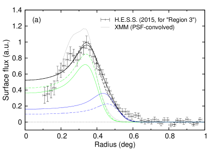
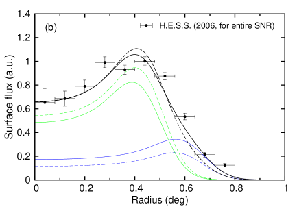
Figure 3: (a) TeV $\gamma$-ray radial surface brightness profile of sector “region 3.” The HESS flux data and the XMM-Newton X-ray brightness profile convolved with the HESS PSF of $3^{\prime}$ (gray line) are adopted from de Naurois (2015). The radial profile of “region 3” is fitted with a two-zone emission (in black), which is the sum of the inner (in green) and outer (in blue) components. The solid and dashed lines represent the profiles in Model Ia and Model IIa, respectively. All of the fitting profile lines have been convolved with the HESS PSF of $3^{\prime}$. (b) TeV $\gamma$-ray radial surface brightness profile for the entire remnant. The HESS flux data are adopted from Aharonian et al. (2006). The meanings of all lines convolved with the HESS PSF of $5^{\prime}$ are the same as those in (a).

References

- Abdo et al. (2010) Abdo, A. A., Ackermann, M., Ajello, M., et al. 2010, ApJ, 710, L92
- Abdo et al. (2011) Abdo, A. A., Ackermann, M., Ajello, M., et al. 2011, ApJ, 734, 28
- Acero et al. (2009) Acero, F., Ballet, J., Decourchelle, A., et al. 2009, A&A, 505, 157
- Ackermann et al. (2013) Ackermann, M., Ajello, M., Allafort, A., et al. 2013, Sci, 339, 807
- Aharonian et al. (2006) Aharonian, F., Akhperjanian, A. G., Bazer-Bachi, A. R., et al. 2006, A&A, 449, 223
- Aharonian et al. (2007) Aharonian, F., Akhperjanian, A. G., Bazer-Bachi, A. R., et al. 2007, A&A, 464, 235
- Aharonian et al. (2011) Aharonian, F., Akhperjanian, A. G., Bazer-Bachi, A. R., et al. 2011, A&A, 531, C1
- Aharonian & Atoyan (1996) Aharonian, F. A., & Atoyan, A. M. 1996, A&A, 309, 917
- Aharonian et al. (2004) Aharonian, F. A., Akhperjanian, A. G., Aye, K.-M., et al. 2004, Nature, 432, 75
- Atoyan et al. (1995) Atoyan, A. M., Aharonian, F. A., & Völk, H. J. 1995, Phys. Rev. D, 52, 3265
- Berezhko & Völk (2008) Berezhko, E. G., & Völk, H. J. 2008, A&A, 492, 695
- Berezinskii et al. (1990) Berezinskii, V. S., Bulanov, S. V., Dogiel, V. A., & Ptuskin, V. S. 1990, Astrophysics of Cosmic Rays (Amsterdam: North-Holland)
- Blandford & Cowie (1982) Blandford, R. D., & Cowie, L. L. 1982, ApJ, 260, 625
- Blumenthal & Gould (1970) Blumenthal, G. R., & Gould, R. J. 1970, RvMP, 42, 237
- Cardillo et al. (2014) Cardillo, M., Tavani, M., Giuliani, A., et al. 2014, A&A, 565, A74
- Cassam-Chenaï et al. (2004) Cassam-Chenaï, G., Decourchelle, A., Ballet, J., et al. 2004, A&A, 427, 199
- Chen et al. (2013) Chen, Y., Zhou, P., & Chu, Y.-H. 2013, ApJ, 769, L16
- Chevalier (1982) Chevalier, R. A. 1982, ApJ, 258, 790
- de Naurois (2015) de Naurois, M. 2015, arXiv:1510.00635
- Ellison et al. (2012) Ellison, D. C., Slane, P., Patnaude, D. J., & Bykov, A. M. 2012, ApJ, 744, 39
- Enomoto et al. (2002) Enomoto, R., Tanimori, T., Naito, T., et al. 2002, Nature, 416, 823
- Fan et al. (2010) Fan, Z. H., Liu, S. M., Yuan, Q., & Fletcher, L. 2010, A&A, 517, L4
- Federici et al. (2015) Federici, S., Pohl, M., Telezhinsky, I., Wilhelm, A., & Dwarkadas, V. V. 2015, A&A, 577, A12
- Finke & Dermer (2012) Finke, J. D., & Dermer, C. D. 2012, ApJ, 751, 65
- Fujita et al. (2010) Fujita, Y., Ohira, Y., & Takahara, F. 2010, ApJ, 712, L153
- Fukui et al. (2003) Fukui, Y., Moriguchi, Y., Tamura, K., et al. 2003, PASJ, 55, L61
- Fukui et al. (2012) Fukui, Y., Sano, H., Sato, J., et al. 2012, ApJ, 746, 82
- Gabici & Aharonian (2014) Gabici, S., & Aharonian, F. A. 2014, MNRAS, 445, L70
- Gabici et al. (2009) Gabici, S., Aharonian, F. A., & Casanova, S. 2009, MNRAS, 396, 1629
- Gamerman (1997) Gamerman, D. 1997, Markov Chain Monte Carlo: Stochastic Simulation for Bayesian Inference (Chapman and Hall, London)
- Giuliani et al. (2011) Giuliani, A., Cardillo, M., Tavani, M., et al. 2011, ApJ, 742, L30
- Inoue et al. (2012) Inoue, T., Yamazaki, R., Inutsuka, S.-i., & Fukui, Y. 2012, ApJ, 744, 71
- Jiang et al. (2010) Jiang, B., Chen, Y., Wang, J., et al. 2010, ApJ, 712, 1147
- Katz & Waxman (2008) Katz, B., & Waxman, E. 2008, J. Cosmology Astropart. Phys, 1, 18
- Kelner et al. (2006) Kelner, S. R., Aharonian, F. A., & Bugayov, V. V. 2006, Phys. Rev. D, 74, 034018
- Koyama et al. (1997) Koyama, K., Kinugasa, K., Matsuzaki, K., et al. 1997, PASJ, 49, L7
- Lee et al. (2012) Lee, S.-H., Ellison, D. C., & Nagataki, S. 2012, ApJ, 750, 156
- Lemoine-Goumard (2015) Lemoine-Goumard, M. 2015, arXiv:1510.01373
- Lewis & Bridle (2002) Lewis, A., & Bridle, S. 2002, Phys. Rev. D, 66, 103511
- Li & Chen (2010) Li, H., & Chen, Y. 2010, MNRAS, 409, L35
- Li & Chen (2012) Li, H., & Chen, Y. 2012, MNRAS, 421, 935
- Li et al. (2011) Li, H., Liu, S., & Chen, Y. 2011, ApJ, 742, L10
- Liu et al. (2008) Liu, S., Fan, Z.-H., Fryer, C. L., Wang, J.-M., & Li, H. 2008, ApJ, 683, L163
- Mackay (2003) Mackay, D. J. C. 2003, Information Theory, Inference and Learning Algorithms (Cambridge: Cambridge University Press)
- Mori (2009) Mori, M. 2009, APh, 31, 341
- Moriguchi et al. (2005) Moriguchi, Y., Tamura, K., Tawara, Y., et al. 2005, ApJ, 631, 947
- Morlino et al. (2009) Morlino, G., Amato, E., & Blasi, P. 2009, MNRAS, 392, 240
- Nava & Gabici (2013) Nava, L., & Gabici, S. 2013, MNRAS, 429, 1643
- Neal (1993) Neal, R. M. 1993, Probabilistic Inference Using Markov Chain Monte Carlo Methods (Department of Computer Science, University of Toronto)
- Ohira et al. (2011) Ohira, Y., Murase, K., & Yamazaki, R. 2011, MNRAS, 410, 1577
- Ohira et al. (2012) Ohira, Y., Yamazaki, R., Kawanaka, N., & Ioka, K. 2012, MNRAS, 427, 91
- Pfeffermann & Aschenbach (1996) Pfeffermann, E., & Aschenbach, B. 1996, Roentgenstrahlung from the Universe, ed. H. U. Zimmermann, J. Trümper, & H. Yorke (MPE Rep. 263; Garching: MPE), 267–268
- Porter et al. (2006) Porter, T. A., Moskalenko, I. V., & Strong, A. W. 2006, ApJ, 648, L29
- Sano et al. (2010) Sano, H., Sato, J., Horachi, H., et al. 2010, ApJ, 724, 59
- Sano et al. (2013) Sano, H., Tanaka, T., Torii, K., et al. 2013, ApJ, 778, 59
- Slane et al. (1999) Slane, P., Gaensler, B. M., Dame, T. M., et al. 1999, ApJ, 525, 357
- Tanaka et al. (2008) Tanaka, T., Uchiyama, Y., Aharonian, F. A., et al. 2008, ApJ, 685, 988
- Tang & Chevalier (2014) Tang, X., & Chevalier, R. A. 2014, ApJ, 784, L35
- Tang & Chevalier (2015) Tang, X., & Chevalier, R. A. 2015, ApJ, 800, 103
- Uchiyama et al. (2010) Uchiyama, Y., Blandford, R. D., Funk, S., Tajima, H., & Tanaka, T. 2010, ApJ, 723, L122
- Uchiyama et al. (2012) Uchiyama, Y., Funk, S., Katagiri, H., et al. 2012, ApJ, 749, L35
- Wang et al. (1997) Wang, Z. R., Qu, Q.-Y., & Chen, Y. 1997, A&A, 318, L59
- Yuan et al. (2011) Yuan, Q., Liu, S., Fan, Z., Bi, X., & Fryer, C. L. 2011, ApJ, 735, 120
- Zhang et al. (2013) Zhang, X., Chen, Y., Li, H., & Zhou, X. 2013, MNRAS, 429, L25
- Zirakashvili & Aharonian (2010) Zirakashvili, V. N., & Aharonian, F. A. 2010, ApJ, 708, 965