Sequence Set Design With Good Correlation Properties via Majorization-Minimization

Abstract

Sets of sequences with good correlation properties are desired in many active sensing and communication systems, e.g., multiple-input–multiple-output (MIMO) radar systems and code-division multiple-access (CDMA) cellular systems. In this paper, we consider the problems of designing complementary sets of sequences (CSS) and also sequence sets with both good auto- and cross-correlation properties. Algorithms based on the general majorization-minimization method are developed to tackle the optimization problems arising from the sequence set design problems. All the proposed algorithms can be implemented by means of the fast Fourier transform (FFT) and thus are computationally efficient and capable of designing sets of very long sequences. A number of numerical examples are provided to demonstrate the performance of the proposed algorithms.

I Introduction

Sequences with good correlation properties play an important role in many active sensing and communication systems[1, 2]. The design of a single sequence with good autocorrelation properties (e.g., small autocorrelation sidelobes) has been studied extensively, e.g., see [3, 4, 5] and the references therein. In this paper, we focus on the design of sets of sequences with good correlation properties. We consider both the design of complementary sets of sequences (CSS) and the design of sequence sets with good auto- and cross-correlation properties. In addition, in order to avoid non-linear side effects and make full use of the transmission power available in the system, we restrict our design to unimodular sequences.

Let $\{\mathbf{x}_{m}\}_{m=1}^{M}$ denote a set of $M$ complex unimodular sequences each of length $N$, i.e., $\mathbf{x}_{m}=[x_{m}(1),\ldots,x_{m}(N)]^{T}$, $m=1,\ldots,M$. Then the aperiodic cross-correlation of $\mathbf{x}_{i}$ and $\mathbf{x}_{j}$ at lag $k$ is defined as

$$r_{i,j}(k) = \sum_{n=1}^{N-k}x_{i}(n+k)x_{j}^{*}(n)=r_{j,i}^{*}(-k),$$ (1)

$$i,j=1,\ldots,M,k=1-N,\ldots,N-1.$$

When $i=j,$ (1) reduces to the autocorrelation of $\mathbf{x}_{i}$.

The motivation of CSS design comes from the difficulties in designing a single unimodular sequence with impulse-like autocorrelation. For instance, it can be easily observed that the autocorrelation sidelobe at lag $N-1$ of a unimodular sequence is always equal to 1, no matter how we design the sequence. The difficulties have encouraged researchers to consider the idea of CSS, and the set of sequences $\{\mathbf{x}_{m}\}_{m=1}^{M}$ is called complementary if and only if the autocorrelations of $\{\mathbf{x}_{m}\}$ sum up to zero at any out-of-phase lag, i.e.,

$$\sum_{m=1}^{M}r_{m,m}(k)=0,\,1\leq\left|k\right|\leq N-1.$$ (2)

CSS have been applied in many active sensing and communication systems, for instance, multiple-input–multiple-output (MIMO) radars [6], radar pulse compression [7], orthogonal frequency-division multiplexing (OFDM) [8], ultra wide-band (UWB) communications [9], code-division multiple-access (CDMA) [10], and channel estimation [11]. Owing to the practical importance, a lot of effort has been devoted to the construction of CSS. The majority of research results on CSS at the early stage have been concerned with the analytical construction of CSS for restricted sequence length $N$ and set cardinality $M$. More recently, computational methods have also been proposed for the design of CSS, see [12] for example. In contrast to analytical constructions, computational methods are more flexible in the sense that they do not impose any restriction on the length of sequences or the set cardinality.

In CSS design, only the autocorrelation properties of the sequences have been considered. But some applications require a set of sequences with not only good autocorrelation properties but also good cross-correlations among the sequences, for example, in CDMA cellular networks or in MIMO radar systems. Good autocorrelation indicates that a sequence is nearly uncorrelated with its own time-shifted versions, while good cross-correlation means that any sequence is nearly uncorrelated with all other time-shifted sequences. Good correlation properties in the above sense ensure that matched filters at the receiver end can easily separate the users in a CDMA system [13] or extract the signals backscattered from the range of interest while attenuating signals backscattered from other ranges in MIMO radar [14].

Extending the approaches in [5], we present in this paper several new algorithms for the design of complementary sets of sequences and sequence sets with both good auto- and cross-correlation properties. The sequence set design problems are first formulated as optimization problems and they include the single sequence design problems considered in [4, 5] as special cases. Then several efficient algorithms are developed based on the general majorization-minimization (MM) method via successively majorizing the objective functions twice. All the proposed algorithms can be implemented by means of the fast Fourier transform (FFT) and are thus very efficient in practice. The convergence properties and an acceleration scheme, which can be used to further accelerate the proposed MM algorithms, are also briefly discussed.

The remaining sections of the paper are organized as follows. In Section II, the problem formulations are presented. In Section III, an MM algorithm is derived for the CSS design problem, followed by the derivations of two MM algorithms for designing sequence sets with good auto- and cross-correlations in Sections IV and V, respectively. Convergence analysis and an acceleration scheme are introduced in Section VI. Finally, Section VII presents some numerical results, and the conclusions are given in Section VIII.

Notation: Boldface upper case letters denote matrices, boldface lower case letters denote column vectors, and italics denote scalars. $\mathbb{R}$ and $\mathbb{C}$ denote the real field and the complex field, respectively. $\mathrm{Re}(\cdot)$ and $\mathrm{Im}(\cdot)$ denote the real and imaginary part, respectively. ${\rm arg}(\cdot)$ denotes the phase of a complex number. The superscripts $(\cdot)^{T}$, $(\cdot)^{*}$ and $(\cdot)^{H}$ denote transpose, complex conjugate, and conjugate transpose, respectively. $X_{i,j}$ denotes the (i-th, j-th) element of matrix $\mathbf{X}$ and $x_{i}$ ($x(i)$) denotes the i-th element of vector $\mathbf{x}$. $\mathbf{X}_{i,:}$ denotes the i-th row of matrix $\mathbf{X}$, $\mathbf{X}_{:,j}$ denotes the j-th column of matrix $\mathbf{X}$, and $\mathbf{X}_{i:j,k:l}$ denotes the submatrix of $\mathbf{X}$ from $X_{i,k}$ to $X_{j,l}$. $\circ$ denotes the Hadamard product. $\otimes$ denotes the Kronecker product. $\mathrm{Tr}(\cdot)$ denotes the trace of a matrix. ${\rm diag}(\mathbf{X})$ is a column vector consisting of all the diagonal elements of $\mathbf{X}$. ${\rm Diag}(\mathbf{x})$ is a diagonal matrix formed with $\mathbf{x}$ as its principal diagonal. ${\rm vec}(\mathbf{X})$ is a column vector consisting of all the columns of $\mathbf{X}$ stacked. $\mathbf{I}_{n}$ denotes an $n\times n$ identity matrix.

II Problem Formulation and MM Primer

The problems of interest in this paper are the design of complementary sets of sequences (CSS) and the design of sequence sets with good auto- and cross-correlation properties. In the following, we first provide criteria to measure the complementarity of a sequence set and also the goodness of auto- and cross-correlation properties respectively, and then formulate the sequence set design problems as optimization problems. The MM method is also briefly introduced, which will be applied to tackle the optimization problems later.

II-A Design of Complementary Set of Sequences

We are interested in developing efficient optimization methods for the design of complementary sets of sequences. Consequently, to measure the complementarity of a sequence set $\{\mathbf{x}_{m}\}_{m=1}^{M}$, we consider the complementary integrated sidelobe level (CISL) metric of a set of sequences, which is defined as

$${\rm CISL}=\sum_{k=1}^{N-1}\left|\sum_{m=1}^{M}r_{m,m}(k)\right|^{2}.$$ (3)

Then a natural idea to generate complementary sets of unimodular sequences is to minimize the CISL metric in (3), i.e., solving the following optimization problem:

$$\begin{array}[]{ll}\underset{\{\mathbf{x}_{m}\}_{m=1}^{M}}{\mathsf{minimize}}&{\displaystyle\sum_{k=1}^{N-1}}\left|{\displaystyle\sum_{m=1}^{M}}r_{m,m}(k)\right|^{2}\\ \mathsf{subject\;to}&\left|x_{m}(n)\right|=1,\\ &n=1,\ldots,N,\,m=1,\ldots,M.\end{array}$$ (4)

Note that if the objective of problem (4) can be driven to zero, then the corresponding solution is a complementary set of sequences. But the problem may also be used to find almost complementary sets of sequences for $(N,M)$ values for which no CSS exists.

II-B Design of Sequence Set with Good Auto- and Cross-correlation Properties

To design sequence sets with both good auto- and cross-correlation properties, we consider the goodness measure used in [14], which is defined as

$$\Psi={\displaystyle\sum_{m=1}^{M}}{\displaystyle\sum_{\begin{subarray}{c}k=1-N\\ k\neq 0\end{subarray}}^{N-1}}\left|r_{m,m}(k)\right|^{2}+{\displaystyle\sum_{i=1}^{M}}{\displaystyle\sum_{\begin{subarray}{c}j=1\\ j\neq i\end{subarray}}^{M}}{\displaystyle\sum_{k=1-N}^{N-1}}\left|r_{i,j}(k)\right|^{2}.$$ (5)

In this criterion, the first term contains the autocorrelation sidelobes of all the sequences and the cross-correlations are involved in the second term. Then, to design unimodular sequence sets with good correlation properties, we consider the following optimization problem:

$$\begin{array}[]{ll}\underset{\{\mathbf{x}_{m}\}_{m=1}^{M}}{\mathsf{minimize}}&{\displaystyle\sum_{m=1}^{M}}{\displaystyle\sum_{\begin{subarray}{c}k=1-N\\ k\neq 0\end{subarray}}^{N-1}}\left|r_{m,m}(k)\right|^{2}+{\displaystyle\sum_{i=1}^{M}}{\displaystyle\sum_{\begin{subarray}{c}j=1\\ j\neq i\end{subarray}}^{M}}{\displaystyle\sum_{k=1-N}^{N-1}}\left|r_{i,j}(k)\right|^{2}\\ \mathsf{subject\;to}&\left|x_{m}(n)\right|=1,\,n=1,\ldots,N,\,m=1,\ldots,M.\end{array}$$ (6)

Since $r_{m,m}(0)=N$, $m=1,\ldots,M$, due to the unimodular constraints, problem (6) can be written more compactly as

$$\begin{array}[]{ll}\underset{\{\mathbf{x}_{m}\}_{m=1}^{M}}{\mathsf{minimize}}&{\displaystyle\sum_{i=1}^{M}}{\displaystyle\sum_{\begin{subarray}{c}j=1\end{subarray}}^{M}}{\displaystyle\sum_{k=1-N}^{N-1}}\left|r_{i,j}(k)\right|^{2}-N^{2}M\\ \mathsf{subject\;to}&\left|x_{m}(n)\right|=1,\\ &n=1,\ldots,N,\,m=1,\ldots,M.\end{array}$$ (7)

As have been shown in [1], the criterion $\Psi$ defined in (5) is lower bounded by $N^{2}M(M-1)$ and thus cannot be made very small. This unveils the fact that it is not possible to design a set of sequences with all auto- and cross-correlation sidelobes very small. Therefore, we also consider the following more general weighted formulation:

$$\begin{array}[]{ll}\underset{\{\mathbf{x}_{m}\}_{m=1}^{M}}{\mathsf{minimize}}&{\displaystyle\sum_{i=1}^{M}}{\displaystyle\sum_{\begin{subarray}{c}j=1\end{subarray}}^{M}}{\displaystyle\sum_{k=1-N}^{N-1}}w_{k}\left|r_{i,j}(k)\right|^{2}-w_{0}N^{2}M\\ \mathsf{subject\;to}&\left|x_{m}(n)\right|=1,\,n=1,\ldots,N,\,m=1,\ldots,M,\end{array}$$ (8)

where $w_{k}=w_{-k}\geq 0$, $k=0,\ldots,N-1$ are nonnegative weights assigned to different time lags. It is easy to see that if we choose $w_{k}=1$ for all $k,$ then problem (8) reduces to (7). But problem (8) provides more flexibility in the sense that we can assign different weights to different correlation lags, so that we can minimize the correlations only within a certain time lag interval. Also note that when $M=1$, problem (8) becomes the weighted integrated sidelobe level minimization problem considered in [5].

Two algorithms named CAN and WeCAN were proposed in [14] to tackle problems (8) and (7), respectively. But the authors of [14] resorted to solving “almost equivalent” problems that seem to work well in practice. In this paper, we develop algorithms to directly tackle the sequence set design formulations in (8) and (7).

II-C The MM Method

The MM method refers to the majorization-minimization method, which is an approach to solve optimization problems that are too difficult to solve directly. The principle behind the MM method is to transform a difficult problem into a series of simple problems. Interested readers may refer to [15, 16, 17] and references therein for more details.

Suppose we want to minimize $f(\mathbf{x})$ over $\mathcal{X}\subseteq\mathbb{C}^{n}$. Instead of minimizing the cost function $f(\mathbf{x})$ directly, the MM approach optimizes a sequence of approximate objective functions that majorize $f(\mathbf{x})$. More specifically, starting from a feasible point $\mathbf{x}^{(0)},$ the algorithm produces a sequence $\{\mathbf{x}^{(k)}\}$ according to the following update rule:

$$\mathbf{x}^{(k+1)}\in\underset{\mathbf{x}\in\mathcal{X}}{\arg\min}\,\,u(\mathbf{x},\mathbf{x}^{(k)}),$$ (9)

where $\mathbf{x}^{(k)}$ is the point generated by the algorithm at iteration $k,$ and $u(\mathbf{x},\mathbf{x}^{(k)})$ is the majorization function of $f(\mathbf{x})$ at $\mathbf{x}^{(k)}$. Formally, the function $u(\mathbf{x},\mathbf{x}^{(k)})$ is said to majorize the function $f(\mathbf{x})$ at the point $\mathbf{x}^{(k)}$ if

$$u(\mathbf{x},\mathbf{x}^{(k)}) \geq f(\mathbf{x}),\quad\forall\mathbf{x}\in\mathcal{X},$$ (10)

$$u(\mathbf{x}^{(k)},\mathbf{x}^{(k)}) = f(\mathbf{x}^{(k)}).$$ (11)

In other words, function $u(\mathbf{x},\mathbf{x}^{(k)})$ is an upper bound of $f(\mathbf{x})$ over $\mathcal{X}$ and coincides with $f(\mathbf{x})$ at $\mathbf{x}^{(k)}$.

It is easy to show that with this scheme, the objective value is monotonically decreasing (nonincreasing) at every iteration, i.e.,

$$f(\mathbf{x}^{(k+1)})\leq u(\mathbf{x}^{(k+1)},\mathbf{x}^{(k)})\leq u(\mathbf{x}^{(k)},\mathbf{x}^{(k)})=f(\mathbf{x}^{(k)}).$$ (12)

The first inequality and the third equality follow from the the properties of the majorization function, namely (10) and (11) respectively and the second inequality follows from (9).

To derive MM algorithms in practice, the key step is to find a majorization function of the objective such that the majorized problem is easy to solve. For that purpose, the following result on quadratic upper-bounding will be useful later when constructing simple majorization functions.

Lemma 1 ([4]).

Let $\mathbf{L}$ be an $n\times n$ Hermitian matrix and $\mathbf{M}$ be another $n\times n$ Hermitian matrix such that $\mathbf{M}\succeq\mathbf{L}.$ Then for any point $\mathbf{x}_{0}\in\mathbf{C}^{n}$, the quadratic function $\mathbf{x}^{H}\mathbf{L}\mathbf{x}$ is majorized by $\mathbf{x}^{H}\mathbf{M}\mathbf{x}+2{\rm Re}\left(\mathbf{x}^{H}(\mathbf{L}-\mathbf{M})\mathbf{x}_{0}\right)+\mathbf{x}_{0}^{H}(\mathbf{M}-\mathbf{L})\mathbf{x}_{0}$ at $\mathbf{x}_{0}$.

III Design of Complementary Set of Sequences via MM

To tackle problem (4) via majorization-minimization, we first perform some reformulations. Let us define an auxiliary sequence of length $M(2N-1)$ as follows [12]:

$$\mathbf{z}=[\mathbf{x}_{1}^{T},\mathbf{0}_{N-1}^{T},\ldots,\mathbf{x}_{M}^{T},\mathbf{0}_{N-1}^{T}]^{T},$$ (13)

then the first $N$ aperiodic autocorrelation lags of $\mathbf{z}$ (denoted by $\{r_{z}(k)\}$) can be written as

$$r_{z}(k)=\sum_{m=1}^{M}r_{m,m}(k),\,0\leq k\leq N-1.$$ (14)

Then the sequence set $\{\mathbf{x}_{m}\}_{m=1}^{M}$ is complementary if and only if $\mathbf{z}$ has a zero correlation zone (ZCZ) for lags in the interval $1\leq k\leq N-1$, and the CSS design problem (4) can be reformulated as

$$\begin{array}[]{ll}\underset{\{\mathbf{x}_{m}\}_{m=1}^{M}}{\mathsf{minimize}}&{\displaystyle\sum_{k=1}^{N-1}}\left|r_{z}(k)\right|^{2}\\ \mathsf{subject\;to}&\mathbf{z}=[\mathbf{x}_{1}^{T},\mathbf{0}_{N-1}^{T},\ldots,\mathbf{x}_{M}^{T},\mathbf{0}_{N-1}^{T}]^{T},\\ &\left|x_{m}(n)\right|=1,\,n=1,\ldots,N,\,m=1,\ldots,M.\end{array}$$ (15)

The objective in (15) can be viewed as the weighted ISL metric in [5] of the sequence $\mathbf{z}$ (i.e., $\sum_{k=1}^{M(2N-1)-1}w_{k}\left|r_{z}(k)\right|^{2}$) with weights chosen as

$$w_{k}=\begin{cases}1,&1\leq k\leq N-1\\ 0,&N\leq k\leq M(2N-1)-1.\end{cases}$$ (16)

However, in problem (15), the sequence $\mathbf{z}$ has some special structures and the original weighted ISL minimization algorithm proposed in [5] for designing unimodular sequences cannot be directly applied due to the zeros. But the algorithm can be adapted to take the sequence structure into account and in the following we give a brief derivation of the modified algorithm, which mainly follows from Section III.B in [5].

Similar to Section III.B in [5], we perform two successive majorization steps to problem (15). Let $L=M(2N-1)$ be the length of $\mathbf{z}$, and $\mathbf{U}_{k},\,k=1-L,\ldots,,L-1$ be $L\times L$ Toeplitz matrices with the $k$th diagonal elements being $1$ and $0$ elsewhere, i.e.,

$$\left[\mathbf{U}_{k}\right]_{i,j}=\begin{cases}1&\textrm{if }j-i=k\\ 0&\textrm{if }j-i\neq k,\end{cases}\quad i,j=1,\ldots,L.$$ (17)

Then the autocorrelations $\{r_{z}(k)\}$ of $\mathbf{z}$ can be written in terms of $\mathbf{U}_{k}$ as

$$r_{z}(k)=\mathbf{z}^{H}\mathbf{U}_{k}\mathbf{z},\,k=1-L,\ldots,,L-1.$$ (18)

Then given $\mathbf{z}^{(l)}=[\mathbf{x}_{1}^{(l)T},\mathbf{0}_{N-1}^{T},\ldots,\mathbf{x}_{M}^{(l)T},\mathbf{0}_{N-1}^{T}]^{T}$ at iteration $l$, by using Lemma 1 we can majorize the objective of (15) by a quadratic function as in [5] and the majorized problem after the first majorization step is given by

$$\begin{array}[]{ll}\underset{\{\mathbf{x}_{m}\}_{m=1}^{M}}{\mathsf{minimize}}&\mathbf{z}^{H}\left(\mathbf{R}-(L-1)\mathbf{z}^{(l)}(\mathbf{z}^{(l)})^{H}\right)\mathbf{z}\\ \mathsf{subject\;to}&\mathbf{z}=[\mathbf{x}_{1}^{T},\mathbf{0}_{N-1}^{T},\ldots,\mathbf{x}_{M}^{T},\mathbf{0}_{N-1}^{T}]^{T},\\ &\left|x_{m}(n)\right|=1,\,n=1,\ldots,N,\,m=1,\ldots,M,\end{array}$$ (19)

where

$$\mathbf{R} = {\displaystyle\sum_{\begin{subarray}{c}k=1-L\\ k\neq 0\end{subarray}}^{L-1}}w_{k}r_{z}^{(l)}(-k)\mathbf{U}_{k}$$ (20)

is a Hermitian Toeplitz matrix and $w_{k}=w_{-k}$, $k=1,\ldots,L-1$ are given in (16).

To perform the second majorization step, we first bound the maximum eigenvalue of the matrix $\mathbf{R}-(L-1)\mathbf{z}^{(l)}(\mathbf{z}^{(l)})^{H}$ as in [5], i.e.,

$$\lambda_{{\rm max}}\left(\mathbf{R}-(L-1)\mathbf{z}^{(l)}(\mathbf{z}^{(l)})^{H}\right)\leq\lambda_{u},$$ (21)

where

$$\lambda_{u} = \frac{1}{2}\left(\max_{1\leq i\leq L}\mu_{2i}+\max_{1\leq i\leq L}\mu_{2i-1}\right),$$ (22)

$$\boldsymbol{\mu} = \mathbf{F}\mathbf{c},$$ (23)

$$\mathbf{c} = [0,w_{1}r_{z}^{(l)}(1),\ldots,w_{L-1}r_{z}^{(l)}(L-1),$$ (24)

$$0,w_{L-1}r_{z}^{(l)}(1-L),\ldots,w_{1}r_{z}^{(l)}(-1)]^{T},$$

and the matrix $\mathbf{F}$ in (23) is the $2L\times 2L$ FFT matrix with $F_{m,n}=e^{-j\frac{2mn\pi}{2L}},0\leq m,n<2L$. Then by applying Lemma 1 with $\mathbf{M=}\lambda_{u}\mathbf{I},$ we can obtain the majorized problem of (19) given by

$$\begin{array}[]{ll}\underset{\{\mathbf{x}_{m}\}_{m=1}^{M}}{\mathsf{minimize}}&{\rm Re}\left(\mathbf{z}^{H}\big{(}\mathbf{R}\!-\!(L-1)\mathbf{z}^{(l)}(\mathbf{z}^{(l)})^{H}\!-\!\lambda_{u}\mathbf{I}\big{)}\mathbf{z}^{(l)}\right)\\ \mathsf{subject\;to}&\mathbf{z}=[\mathbf{x}_{1}^{T},\mathbf{0}_{N-1}^{T},\ldots,\mathbf{x}_{M}^{T},\mathbf{0}_{N-1}^{T}]^{T},\\ &\left|x_{m}(n)\right|=1,\,n=1,\ldots,N,\,m=1,\ldots,M,\end{array}$$ (25)

which can be rewritten as

$$\begin{array}[]{ll}\underset{\{\mathbf{x}_{m}\}_{m=1}^{M}}{\mathsf{minimize}}&\left\|\mathbf{z}-\mathbf{y}\right\|_{2}^{2}\\ \mathsf{subject\;to}&\mathbf{z}=[\mathbf{x}_{1}^{T},\mathbf{0}_{N-1}^{T},\ldots,\mathbf{x}_{M}^{T},\mathbf{0}_{N-1}^{T}]^{T},\\ &\left|x_{m}(n)\right|=1,\,n=1,\ldots,N,\,m=1,\ldots,M,\end{array}$$ (26)

where

$$\mathbf{y} = -\big{(}\mathbf{R}-(L-1)\mathbf{z}^{(l)}(\mathbf{z}^{(l)})^{H}-\lambda_{u}\mathbf{I}\big{)}\mathbf{z}^{(l)}$$ (27)

$$= \left((L-1)MN+\lambda_{u}\right)\mathbf{z}^{(l)}-\mathbf{R}\mathbf{z}^{(l)}.$$

Problem (26) admits the following closed form solution

$$x_{m}(n) = e^{j{\rm arg}(y_{(m-1)(2N-1)+n})},$$ (28)

$$n=1,\ldots,N,m=1,\ldots,M.$$

The overall algorithm for the CSS design problem (4) is summarized in Algorithm 1. Note that the algorithm can be implemented by means of FFT (IFFT) operations, since $\mathbf{R}$ is Hermitian Toeplitz and it can be decomposed as

$$\mathbf{R}=\frac{1}{2L}\mathbf{F}_{:,1:L}^{H}{\rm Diag}(\boldsymbol{\mu})\mathbf{F}_{:,1:L},$$ (29)

according to Lemma 4 in [5].

0:   number of sequences $M$, sequence length $N$

1:   Set $l=0$ and initialize $\{\mathbf{x}_{m}^{(0)}\}_{m=1}^{M}$.

2:   $L=M(2N-1)$

3:  repeat

4:      $\mathbf{z}^{(l)}=[\mathbf{x}_{1}^{(l)T},\mathbf{0}_{N-1}^{T},\ldots,\mathbf{x}_{M}^{(l)T},\mathbf{0}_{N-1}^{T}]^{T}$

5:      $\mathbf{f}=\mathbf{F}[\mathbf{z}^{(l)T},\mathbf{0}_{1\times L}]^{T}$

6:      $\mathbf{r}=\frac{1}{2L}\mathbf{F}^{H}\left|\mathbf{f}\right|^{2}$

7:      $\mathbf{c}=\mathbf{r}\circ[0,\mathbf{1}_{N-1}^{T},\mathbf{0}_{2(L-N)+1}^{T},\mathbf{1}_{N-1}^{T}]^{T}$

8:      $\boldsymbol{\mu}=\mathbf{F}\mathbf{c}$

9:      $\lambda_{u}=\frac{1}{2}\big{(}\underset{1\leq i\leq N}{\max}\mu_{2i}+\underset{1\leq i\leq N}{\max}\mu_{2i-1}\big{)}$3

10:      $\mathbf{y}=\left((L-1)MN+\lambda_{u}\right)\mathbf{z}^{(l)}-\frac{1}{2L}\mathbf{F}_{:,1:L}^{H}(\boldsymbol{\mu}\circ\mathbf{f})$

11:      $x_{m}^{(l+1)}(n)=e^{j{\rm arg}(y_{(m-1)(2N-1)+n})},n=1,\ldots,N,m=1,\ldots,M.$

12:      $l\leftarrow l+1$

13:  until  convergence

Algorithm 1 The MM Algorithm for CSS design problem (4).

IV Design of Sequence Set with Good Auto- and Cross-correlation Properties via MM

In this section, we consider the problem of designing sequence sets for both good auto- and cross-correlation properties. We first consider the more general problem formulation with weights involved, i.e., problem (8), and derive an MM algorithm for the problem in the following.

Let us first stack the sequences $\mathbf{x}_{m},m=1,\ldots,M$ together and denote it by $\mathbf{x}$, i.e.,

$$\mathbf{x}=[\mathbf{x}_{1}^{T},\ldots,\mathbf{x}_{M}^{T}]^{T},$$ (30)

then we have

$$\mathbf{x}_{m}=\mathbf{S}_{m}\mathbf{x},\,m=1,\ldots,M,$$ (31)

where $\mathbf{S}_{m}$ is an $N\times NM$ block selection matrix defined as

$$\mathbf{S}_{m}=[\mathbf{0}_{N\times(m-1)N},\mathbf{I}_{N},\mathbf{0}_{N\times(M-m)N}].$$ (32)

We then note that (1) can be written more compactly as

$$r_{i,j}(k)=\mathbf{x}_{j}^{H}\mathbf{U}_{k}\mathbf{x}_{i},\,k=1-N,\ldots,N-1,\,i,j=1,\ldots,M,$$ (33)

where $\mathbf{U}_{k}$ is defined as in (17) but is of size $N\times N$ now. By combining (33) and (31), we have

$$r_{i,j}(k) = \mathbf{x}^{H}\mathbf{S}_{j}^{H}\mathbf{U}_{k}\mathbf{S}_{i}\mathbf{x},$$

$$k=1-N,\ldots,N-1,\,i,j=1,\ldots,M,$$

and then

$$\left|r_{i,j}(k)\right|^{2} =\left|\mathbf{x}^{H}\mathbf{S}_{j}^{H}\mathbf{U}_{k}\mathbf{S}_{i}\mathbf{x}\right|^{2}$$ (35)

$$=\left|{\rm Tr}\left(\mathbf{x}\mathbf{x}^{H}\mathbf{S}_{j}^{H}\mathbf{U}_{k}\mathbf{S}_{i}\right)\right|^{2}$$

$$=\left|{\rm vec}(\mathbf{x}\mathbf{x}^{H})^{H}{\rm vec}(\mathbf{S}_{j}^{H}\mathbf{U}_{k}\mathbf{S}_{i})\right|^{2}.$$

By using (35), problem (8) can be rewritten as

$$\begin{array}[]{ll}\underset{\mathbf{x}\in\mathbb{C}^{NM}}{\mathsf{minimize}}&{\rm vec}(\mathbf{x}\mathbf{x}^{H})^{H}\mathbf{L}{\rm vec}(\mathbf{x}\mathbf{x}^{H})-w_{0}N^{2}M\\ \mathsf{subject\;to}&\left|x_{n}\right|=1,\,n=1,\ldots,NM,\end{array}$$ (36)

where

$$\mathbf{L}={\displaystyle\sum_{i=1}^{M}}{\displaystyle\sum_{\begin{subarray}{c}j=1\end{subarray}}^{M}}{\displaystyle\sum_{k=1-N}^{N-1}}w_{k}{\rm vec}(\mathbf{S}_{j}^{H}\mathbf{U}_{k}\mathbf{S}_{i}){\rm vec}(\mathbf{S}_{j}^{H}\mathbf{U}_{k}\mathbf{S}_{i})^{H}.$$ (37)

Since $w_{k}\geq 0,$ it is easy to see that $\mathbf{L}$ is a nonnegative real symmetric matrix and it can be shown (see Lemma 5 in [5]) that

$$\mathbf{L}\preceq{\rm Diag}(\mathbf{b}),$$ (38)

where $\mathbf{b}=\mathbf{L}\mathbf{1}$. Then given $\mathbf{x}^{(l)}$ at iteration $l$, by using Lemma 1, we know that the objective of problem (36) is majorized by the following function at $\mathbf{x}^{(l)}$:

$$\,\,u_{1}(\mathbf{x},\mathbf{x}^{(l)})$$ (39)

$$= \,\,{\rm vec}(\mathbf{x}\mathbf{x}^{H})^{H}{\rm Diag}(\mathbf{b}){\rm vec}(\mathbf{x}\mathbf{x}^{H})$$

$$+2{\rm Re}\big{(}{\rm vec}(\mathbf{x}\mathbf{x}^{H})^{H}(\mathbf{L}-{\rm Diag}(\mathbf{b})){\rm vec}(\mathbf{x}^{(l)}\mathbf{x}^{(l)H})\big{)}$$

$$+{\rm vec}(\mathbf{x}^{(l)}\mathbf{x}^{(l)H})^{H}({\rm Diag}(\mathbf{b})-\mathbf{L}){\rm vec}(\mathbf{x}^{(l)}\mathbf{x}^{(l)H})-w_{0}N^{2}M.$$

Since the elements of $\mathbf{x}$ are of unit modulus, it is easy to see that the first term of (39) is just a constant. After ignoring the constant terms, the majorized problem of (36) is given by

$$\begin{array}[]{ll}\underset{\mathbf{x}\in\mathbb{C}^{NM}}{\mathsf{minimize}}&{\rm Re}\big{(}{\rm vec}(\mathbf{x}\mathbf{x}^{H})^{H}(\mathbf{L}-{\rm Diag}(\mathbf{b})){\rm vec}(\mathbf{x}^{(l)}\mathbf{x}^{(l)H})\big{)}\\ \mathsf{subject\;to}&\left|x_{n}\right|=1,\,n=1,\ldots,NM.\end{array}$$ (40)

By substituting $\mathbf{L}$ in (37) back, we have

$${\rm Re}\big{(}{\rm vec}(\mathbf{x}\mathbf{x}^{H})^{H}\mathbf{L}{\rm vec}(\mathbf{x}^{(l)}\mathbf{x}^{(l)H})\big{)}$$ (41)

$$= {\displaystyle\sum_{i=1}^{M}}{\displaystyle\sum_{\begin{subarray}{c}j=1\end{subarray}}^{M}}{\displaystyle\sum_{k=1-N}^{N-1}}{\rm Re}\bigg{(}w_{k}{\rm Tr}\left(\mathbf{x}\mathbf{x}^{H}\mathbf{S}_{j}^{H}\mathbf{U}_{k}\mathbf{S}_{i}\right)$$

$$\qquad\qquad\qquad\quad\times{\rm Tr}\left(\mathbf{x}^{(l)}\mathbf{x}^{(l)H}\mathbf{S}_{i}^{H}\mathbf{U}_{-k}\mathbf{S}_{j}\right)\bigg{)}$$

$$= {\displaystyle\sum_{i=1}^{M}}{\displaystyle\sum_{\begin{subarray}{c}j=1\end{subarray}}^{M}}{\displaystyle\sum_{k=1-N}^{N-1}}{\rm Re}\left(w_{k}r_{j,i}^{(l)}(-k)\mathbf{x}^{H}\mathbf{S}_{j}^{H}\mathbf{U}_{k}\mathbf{S}_{i}\mathbf{x}\right),$$

and the second term of the objective can also be rewritten as

$${\rm Re}\big{(}{\rm vec}(\mathbf{x}\mathbf{x}^{H})^{H}{\rm Diag}(\mathbf{b}){\rm vec}(\mathbf{x}^{(l)}\mathbf{x}^{(l)H})\big{)}$$ (42)

$$= {\rm Re}\left({\rm vec}(\mathbf{x}\mathbf{x}^{H})^{H}\left(\mathbf{b}\circ{\rm vec}(\mathbf{x}^{(l)}\mathbf{x}^{(l)H})\right)\right)$$

$$= {\rm Re}\left({\rm Tr}\left(\mathbf{x}\mathbf{x}^{H}{\rm mat}\left(\mathbf{b}\circ{\rm vec}(\mathbf{x}^{(l)}\mathbf{x}^{(l)H})\right)\right)\right)$$

$$= {\rm Re}\left(\mathbf{x}^{H}\left({\rm mat}(\mathbf{b})\circ(\mathbf{x}^{(l)}\mathbf{x}^{(l)H})\right)\mathbf{x}\right),$$

where ${\rm mat}(\cdot)$ is the inverse operation of ${\rm vec}(\cdot)$. It is clear that both (41) and (42) are quadratic in $\mathbf{x}$ and problem (40) can be rewritten as

$$\begin{array}[]{ll}\underset{\mathbf{x}\in\mathbb{C}^{NM}}{\mathsf{minimize}}&\mathbf{x}^{H}\left(\mathbf{R}-\mathbf{B}\circ\big{(}\mathbf{x}^{(l)}(\mathbf{x}^{(l)})^{H}\big{)}\right)\mathbf{x}\\ \mathsf{subject\;to}&\left|x_{n}\right|=1,\,n=1,\ldots,NM,\end{array}$$ (43)

where

$$\mathbf{R}={\displaystyle\sum_{i=1}^{M}}{\displaystyle\sum_{\begin{subarray}{c}j=1\end{subarray}}^{M}}{\displaystyle\sum_{k=1-N}^{N-1}}w_{k}r_{j,i}^{(l)}(-k)\mathbf{S}_{j}^{H}\mathbf{U}_{k}\mathbf{S}_{i},$$ (44)

$$\mathbf{B} ={\rm mat}(\mathbf{b})$$ (45)

$$={\rm mat}(\mathbf{L}\mathbf{1})$$

$$={\rm mat}\left({\displaystyle\sum_{i=1}^{M}}{\displaystyle\sum_{\begin{subarray}{c}j=1\end{subarray}}^{M}}{\displaystyle\sum_{k=1-N}^{N-1}}w_{k}{\rm vec}(\mathbf{S}_{j}^{H}\mathbf{U}_{k}\mathbf{S}_{i}){\rm vec}(\mathbf{S}_{j}^{H}\mathbf{U}_{k}\mathbf{S}_{i})^{H}\mathbf{1}\right)$$

$$={\rm mat}\left({\displaystyle\sum_{i=1}^{M}}{\displaystyle\sum_{\begin{subarray}{c}j=1\end{subarray}}^{M}}{\displaystyle\sum_{k=1-N}^{N-1}}w_{k}(N-\left|k\right|){\rm vec}(\mathbf{S}_{j}^{H}\mathbf{U}_{k}\mathbf{S}_{i})\right)$$

$$={\displaystyle\sum_{i=1}^{M}}{\displaystyle\sum_{\begin{subarray}{c}j=1\end{subarray}}^{M}}{\displaystyle\sum_{k=1-N}^{N-1}}w_{k}(N-\left|k\right|)\mathbf{S}_{j}^{H}\mathbf{U}_{k}\mathbf{S}_{i}$$

$$=\mathbf{1}_{M\times M}\otimes\mathbf{W},$$

and

$$\mathbf{W} ={\displaystyle\sum_{k=1-N}^{N-1}}w_{k}(N-\left|k\right|)\mathbf{U}_{k}$$

$$=\begin{bmatrix}w_{0}N&w_{1}(N-1)&\ldots&w_{N-1}\\ w_{1}(N-1)&w_{0}N&\ddots&\vdots\\ \vdots&\ddots&\ddots&w_{1}(N-1)\\ w_{N-1}&\ldots&w_{1}(N-1)&w_{0}N\end{bmatrix}.$$

Note that in (43) we have removed the ${\rm Re}(\cdot)$ operator since the matrices $\mathbf{R}$ and $\mathbf{B}$ are Hermitian. Since the majorized problem (43) is still hard to solve directly, we propose to majorize the objective function at $\mathbf{x}^{(l)}$ again to further simplify the problem that we need to solve at each iteration. Similarly, to construct a majorization function of the quadratic objective in (43), we need to find a matrix $\mathbf{M}$ such that $\mathbf{M}\succeq\mathbf{R}-\mathbf{B}\circ\big{(}\mathbf{x}^{(l)}(\mathbf{x}^{(l)})^{H}\big{)}$ and a straightforward choice may be $\mathbf{M}=\lambda_{{\rm max}}\left(\mathbf{R}-\mathbf{B}\circ\big{(}\mathbf{x}^{(l)}(\mathbf{x}^{(l)})^{H}\big{)}\right)\mathbf{I}$. But to compute the maximum eigenvalue, some iterative algorithms are needed and since we need to compute this at every iteration, it will be computationally expensive. To maintain the computational efficiency of the algorithm, here we propose to use some upper bound of $\lambda_{{\rm max}}\left(\mathbf{R}-\mathbf{B}\circ\big{(}\mathbf{x}^{(l)}(\mathbf{x}^{(l)})^{H}\big{)}\right)$ that can be easily computed. To derive such an upper bound, we first introduce several results that will be useful. The first result reveals a fact regarding the eigenvalues of the matrix $\mathbf{B}\circ\big{(}\mathbf{x}^{(l)}(\mathbf{x}^{(l)})^{H}\big{)}$, which follows from [5].

Lemma 2.

Let $\mathbf{B}$ be an $N\times N$ matrix and $\mathbf{x}\in\mathbb{C}^{N}$ with $\left|x_{n}\right|=1,\,n=1,\ldots,N$. Then $\mathbf{B}\circ(\mathbf{x}\mathbf{x}^{H})$ and $\mathbf{B}$ share the same set of eigenvalues.

The second result indicates some relations between the eigenvalues of the Kronecker product of two matrices and the eigenvalues of the two individual matrices [18].

Lemma 3.

Let $\mathbf{A}$ and $\mathbf{B}$ be square matrices of size $M$ and $N$, respectively. Let $\lambda_{1},\ldots,\lambda_{M}$ be the eigenvalues of $\mathbf{A}$ and $\mu_{1},\ldots,\mu_{N}$ be those of $\mathbf{B}$. Then the eigenvalues of $\mathbf{A}\otimes\mathbf{B}$ are $\lambda_{i}\mu_{j},i=1,\ldots,M$, $j=1,\ldots,N$ (including algebraic multiplicities in all three cases).

The third result regards bounds of the extreme eigenvalues of Hermitian Toeplitz matrices, which can be computed by using FFTs [19].

Lemma 4.

Let $\mathbf{T}$ be an $N\times N$ Hermitian Toeplitz matrix defined by $\{t_{k}\}_{k=0}^{N-1}$ as follows:

$$\mathbf{T}=\begin{bmatrix}t_{0}&t_{1}^{*}&\ldots&t_{N-1}^{*}\\ t_{1}&t_{0}&\ddots&\vdots\\ \vdots&\ddots&\ddots&t_{1}^{*}\\ t_{N-1}&\ldots&t_{1}&t_{0}\end{bmatrix}$$

and $\mathbf{F}$ be a $2N\times 2N$ FFT matrix with $F_{m,n}=e^{-j\frac{2mn\pi}{2N}},0\leq m,n<2N$. Let $\mathbf{c}=[t_{0},t_{1},\cdots,t_{N-1},0,t_{N-1}^{*},\cdots,t_{1}^{*}]^{T}$ and $\boldsymbol{\mu}=\mathbf{F}\mathbf{c}$ be the discrete Fourier transform of $\mathbf{c}$. Then

$$\lambda_{{\rm max}}(\mathbf{T}) \leq \frac{1}{2}\left(\max_{1\leq i\leq N}\mu_{2i}+\max_{1\leq i\leq N}\mu_{2i-1}\right),$$ (46)

$$\lambda_{{\rm min}}(\mathbf{T}) \geq \frac{1}{2}\left(\min_{1\leq i\leq N}\mu_{2i}+\min_{1\leq i\leq N}\mu_{2i-1}\right).$$ (47)

Based on these results, we can now obtain an upper bound of $\lambda_{{\rm max}}\left(\mathbf{R}-\mathbf{B}\circ\big{(}\mathbf{x}^{(l)}(\mathbf{x}^{(l)})^{H}\big{)}\right)$ given in the following lemma.

Lemma 5.

Let $\mathbf{R}$ and $\mathbf{B}$ be matrices defined in (44) and (45), respectively. Let $\mathbf{w}=[w_{0}N,w_{1}(N-1),\ldots,w_{N-1},0,w_{N-1},\ldots,w_{1}(N-1)]^{T},$ $\boldsymbol{\mu}=\mathbf{F}\mathbf{w}$ and $\lambda_{W}=\frac{1}{2}\left(\min_{1\leq i\leq N}\mu_{2i}+\min_{1\leq i\leq N}\mu_{2i-1}\right)$. Then

$$\lambda_{{\rm max}}\left(\mathbf{R}-\mathbf{B}\circ\big{(}\mathbf{x}^{(l)}(\mathbf{x}^{(l)})^{H}\big{)}\right)\leq\left\|\mathbf{R}\right\|-\lambda_{B},$$ (48)

where

$$\lambda_{B}=\begin{cases}\min\left\{M\lambda_{W},0\right\},&M\geq 2\\ \lambda_{W},&M=1,\end{cases}$$ (49)

and $\left\|\cdot\right\|$ can be any submultiplicative matrix norm.

Proof:

See Appendix A. ∎

In our case, for computational efficiency, we choose the induced $\ell_{\infty}$-norm (also known as max-row-sum norm) in Lemma 5, which is defined as

$$\left\|\mathbf{R}\right\|_{\infty}=\max_{i=1,\ldots,NM}\sum_{j=1}^{NM}\left|R_{i,j}\right|.$$ (50)

Now, by choosing $\mathbf{M}=\left(\left\|\mathbf{R}\right\|_{\infty}-\lambda_{B}\right)\mathbf{I}$ in Lemma 1, the objective in (43) is majorized by

$$\,\,u_{2}(\mathbf{x},\mathbf{x}^{(l)})$$

$$= \,\,(\left\|\mathbf{R}\right\|_{\infty}-\lambda_{B})\mathbf{x}^{H}\mathbf{x}$$

$$+2{\rm Re}\left(\mathbf{x}^{H}\big{(}\mathbf{R}\!-\!\mathbf{B}\circ\big{(}\mathbf{x}^{(l)}(\mathbf{x}^{(l)})^{H}\big{)}\!-\!(\left\|\mathbf{R}\right\|_{\infty}\!-\!\lambda_{B})\mathbf{I}\big{)}\mathbf{x}^{(l)}\right)$$

$$+(\mathbf{x}^{(l)})^{H}((\left\|\mathbf{R}\right\|_{\infty}-\lambda_{B})\mathbf{I}-\mathbf{R}\!+\!\mathbf{B}\circ\big{(}\mathbf{x}^{(l)}(\mathbf{x}^{(l)})^{H}\big{)})\mathbf{x}^{(l)}.$$

Again after ignoring the constant terms, the majorized problem of (43) is given by

$$\begin{array}[]{ll}\underset{\mathbf{x}\in\mathbb{C}^{NM}}{\mathsf{minimize}}&{\rm Re}\left(\mathbf{x}^{H}\mathbf{y}\right)\\ \mathsf{subject\;to}&\left|x_{n}\right|=1,\,n=1,\ldots,NM,\end{array}$$ (51)

where

$$\mathbf{y}=\big{(}\mathbf{R}\!-\!\mathbf{B}\circ\big{(}\mathbf{x}^{(l)}(\mathbf{x}^{(l)})^{H}\big{)}\big{)}\mathbf{x}^{(l)}\!-\!(\left\|\mathbf{R}\right\|_{\infty}\!-\!\lambda_{B})\mathbf{x}^{(l)}.$$ (52)

It is clear that problem (51) is separable in the elements of $\mathbf{x}$ and the solution of the problem is given by

$$x_{n}=e^{j{\rm arg}(-y_{n})},n=1,\ldots,NM.$$ (53)

According to the general steps of the majorization minimization method, we can now implement the algorithm in a straightforward way, that is at each iteration, we compute $\mathbf{y}$ according to (52) and update $\mathbf{x}$ via (53). Clearly, the computational cost is dominated by the computation of $\mathbf{y}$. To obtain an efficient implementation, here we further explore the special structure of the matrices involved in the computation of $\mathbf{y}$.

We first note that the matrix $\mathbf{R}$ in (44) can be written as the following block matrix:

$$\mathbf{R}=\begin{bmatrix}\mathbf{R}_{11}&\mathbf{R}_{12}&\cdots&\mathbf{R}_{1M}\\ \mathbf{R}_{21}&\mathbf{R}_{22}&\cdots&\mathbf{R}_{2M}\\ \vdots&\vdots&\ddots&\vdots\\ \mathbf{R}_{M1}&\cdots&\cdots&\mathbf{R}_{MM}\end{bmatrix},$$ (54)

where each block is defined as

$$\mathbf{R}_{ij}={\displaystyle\sum_{k=1-N}^{N-1}}w_{k}r_{i,j}^{(l)}(-k)\mathbf{U}_{k},\,i,j=1,\ldots,M.$$ (55)

It is easy to see that the building blocks $\mathbf{R}_{ij},i,j=1,\ldots,M$, are Toeplitz matrices and when $i=j,$ they are also Hermitian. In the following, we introduce a simple result regarding Toeplitz matrices (not necessarily Hermitian) that can be used to perform the matrix vector multiplication $\mathbf{R}\mathbf{x}^{(l)}$ more efficiently via FFT (IFFT).

Lemma 6.

Let $\mathbf{T}$ be an $N\times N$ Toeplitz matrix defined as follows:

$$\mathbf{T}=\begin{bmatrix}t_{0}&t_{1}&\ldots&t_{N-1}\\ t_{-1}&t_{0}&\ddots&\vdots\\ \vdots&\ddots&\ddots&t_{1}\\ t_{1-N}&\ldots&t_{-1}&t_{0}\end{bmatrix}$$

and $\mathbf{F}$ be a $2N\times 2N$ FFT matrix with $F_{m,n}=e^{-j\frac{2mn\pi}{2N}},0\leq m,n<2N$. Then $\mathbf{T}$ can be decomposed as $\mathbf{T}=\frac{1}{2N}\mathbf{F}_{:,1:N}^{H}{\rm Diag}(\mathbf{F}\mathbf{c})\mathbf{F}_{:,1:N}$, where $\mathbf{c}=[t_{0},t_{-1},\cdots,t_{1-N},0,t_{N-1},\cdots,t_{1}]^{T}$.

Proof:

See Appendix B. ∎

According to Lemma 6, by defining $\mathbf{H}$ to be the $2N\times N$ matrix composed of the first $N$ columns of the $2N\times 2N$ FFT matrix, i.e.,

$$\mathbf{H}=\mathbf{F}_{:,1:N},$$ (56)

we know that

$$\mathbf{R}_{ij}=\frac{1}{2N}\mathbf{H}^{H}{\rm Diag}(\mathbf{F}\mathbf{c}_{ij})\mathbf{H},$$ (57)

where

$$\mathbf{c}_{ij} =[w_{0}r_{i,j}^{(l)}(0),w_{1}r_{i,j}^{(l)}(1),\ldots,w_{N-1}r_{i,j}^{(l)}(N-1),$$ (58)

$$\quad\,\,\,0,w_{N-1}r_{i,j}^{(l)}(1-N),\ldots,w_{1}r_{i,j}^{(l)}(-1)]^{T}.$$

Thus, the matrix vector multiplication $\mathbf{R}\mathbf{x}^{(l)}$ can be performed as

$$\mathbf{R}\mathbf{x}^{(l)}=\frac{1}{2N}\tilde{\mathbf{H}}^{H}\begin{bmatrix}{\rm Diag}(\mathbf{F}\mathbf{c}_{11})&\cdots&{\rm Diag}(\mathbf{F}\mathbf{c}_{1M})\\ \vdots&\ddots&\vdots\\ {\rm Diag}(\mathbf{F}\mathbf{c}_{M1})&\cdots&{\rm Diag}(\mathbf{F}\mathbf{c}_{MM})\end{bmatrix}\tilde{\mathbf{H}}\mathbf{x}^{(l)},$$ (59)

where $\tilde{\mathbf{H}}$ is a $2MN\times MN$ block diagonal matrix given by

$$\tilde{\mathbf{H}}=\begin{bmatrix}\mathbf{H}&\mathbf{0}&\cdots&\mathbf{0}\\ \mathbf{0}&\mathbf{H}&\ddots&\vdots\\ \vdots&\ddots&\ddots&\mathbf{0}\\ \mathbf{0}&\cdots&\mathbf{0}&\mathbf{H}\end{bmatrix}.$$ (60)

From (59), we can see that the multiplication $\mathbf{R}\mathbf{x}^{(l)}$ takes $M^{2}+2M$ FFT (IFFT) operations if all $\mathbf{c}_{ij},i,j=1,\ldots,M$ are given. Since to form the vectors $\mathbf{c}_{ij},i,j=1,\ldots,M,$ all the autocorrelations and cross-correlations, i.e., $r_{i,j}^{(l)}(k),i,j=1,\ldots,M,\,k=1-N,\ldots,N-1,$ are needed, and another $M^{2}$ FFT (IFFT) operations are required. Similarly, $\left\|\mathbf{R}\right\|_{\infty}$ can also be computed with $M^{2}+2M$ FFT (IFFT) operations, since it can be obtained by taking the largest element of the vector $\tilde{\mathbf{R}}\mathbf{1}$, where $\tilde{\mathbf{R}}$ is the matrix with each element being the modulus of the corresponding element of $\mathbf{R}$, i.e., $\tilde{R}_{i,j}=\left|R_{i,j}\right|,i,j=1,\ldots,N.$ Finally, to compute $\big{(}\mathbf{B}\circ\big{(}\mathbf{x}^{(l)}(\mathbf{x}^{(l)})^{H}\big{)}\big{)}\mathbf{x}^{(l)}$ we first conduct some transformations as follows:

$$\,\,\big{(}\mathbf{B}\circ\big{(}\mathbf{x}^{(l)}(\mathbf{x}^{(l)})^{H}\big{)}\big{)}\mathbf{x}^{(l)}$$ (61)

$$= \,\,{\rm diag}\big{(}\mathbf{B}{\rm Diag}(\mathbf{x}^{(l)})\big{(}\mathbf{x}^{(l)}(\mathbf{x}^{(l)})^{H}\big{)}^{T}\big{)}$$

$$= \,\,{\rm diag}\big{(}\mathbf{B}\big{(}\mathbf{x}^{(l)}\circ\big{(}\mathbf{x}^{(l)}\big{)}^{*})\big{(}\mathbf{x}^{(l)}\big{)}^{T}\big{)}$$

$$= \,\,{\rm diag}\big{(}\mathbf{B}\mathbf{1}_{NM\times 1}\big{(}\mathbf{x}^{(l)}\big{)}^{T}\big{)}$$

$$= \,\,(\mathbf{B}\mathbf{1}_{NM\times 1})\circ\mathbf{x}^{(l)}$$

$$= \,\,\left((\mathbf{1}_{M\times M}\otimes\mathbf{W})\mathbf{1}_{NM\times 1}\right)\circ\mathbf{x}^{(l)}$$

$$= \,\,\left(M\mathbf{1}_{M\times 1}\otimes(\mathbf{W}\mathbf{1}_{N\times 1})\right)\circ\mathbf{x}^{(l)}.$$

Since $\mathbf{W}$ is Toeplitz, we know from Lemma 6 that it can be decomposed as

$$\mathbf{W}=\frac{1}{2N}\mathbf{H}^{H}{\rm Diag}(\mathbf{F}\mathbf{w})\mathbf{H},$$ (62)

where $\mathbf{w}$ is the same as the one defined in Lemma 5. Thus, $\big{(}\mathbf{B}\circ\big{(}\mathbf{x}^{(l)}(\mathbf{x}^{(l)})^{H}\big{)}\big{)}\mathbf{x}^{(l)}$ can be computed with $3$ FFT (IFFT) operations.

In summary, to compute $\mathbf{y}$ as in (52), around $3M^{2}+4M+3$ $2N$-point FFT (IFFT) operations are needed. Since the computational complexity of one FFT (IFFT) is $\mathcal{O}(N\log N),$ the per iteration computational complexity of the proposed algorithm is of order $\mathcal{O}(M^{2}N\log N)$. The overall algorithm is summarized in Algorithm 2.

0:   number of sequences $M$, sequence length $N$, weights $\{w_{k}\geq 0\}_{k=0}^{N-1}$

1:   Set $l=0$, initialize $\mathbf{x}^{(0)}$ of length $MN$.

2:   $\mathbf{w}=[w_{0}N,w_{1}(N-1),\ldots,w_{N-1},0,w_{N-1},\ldots,w_{1}(N-1)]^{T}$

3:   $\boldsymbol{\mu}=\mathbf{F}\mathbf{w}$

4:   $\lambda_{W}=\frac{1}{2}\left({\displaystyle\min_{1\leq i\leq N}}\mu_{2i}+{\displaystyle\min_{1\leq i\leq N}}\mu_{2i-1}\right)$

5:   $\lambda_{B}=\begin{cases}\min\left\{M\lambda_{W},0\right\},&M\geq 2\\ \lambda_{W},&M=1\end{cases}$

6:  repeat

7:      Compute $r_{i,j}^{(l)}(k),i,j=1,\ldots,M,k=1-N,\dots,N-1$.

8:      Compute $\mathbf{c}_{ij},i,j=1,\ldots,M$ according to (58).

9:      Compute $\mathbf{R}\mathbf{x}^{(l)}$ according to (59).

10:      Compute $\left\|\mathbf{R}\right\|_{\infty}$ based on $\left|\mathbf{c}_{ij}\right|,i,j=1,\ldots,M$.

11:      $\mathbf{p}=\frac{M}{2N}\mathbf{1}_{M\times 1}\otimes\left(\mathbf{H}^{H}\left(\boldsymbol{\mu}\circ(\mathbf{H}\mathbf{1})\right)\right)$

12:      $\mathbf{y}=\frac{\mathbf{R}\mathbf{x}^{(l)}-\mathbf{p}\circ\mathbf{x}^{(l)}}{\left\|\mathbf{R}\right\|_{\infty}\!-\!\lambda_{B}}\!-\!\mathbf{x}^{(l)}$

13:      $x_{n}^{(l+1)}=e^{j{\rm arg}(-y_{n})},\,n=1,\ldots,MN$

14:      $l\leftarrow l+1$

15:  until  convergence

Algorithm 2 The MM Algorithm for problem (8).

V Simplified MM for the Case without Weights

In the previous section, we developed an algorithm for problem (8). By simply choosing weights $w_{k}=1,k=1-N,\ldots,1+N$, the algorithm can be readily applied to solve problem (7). However, as analyzed in the previous section, the algorithm requires about $3M^{2}+4M$ $2N$-point FFT (IFFT) operations at every iteration. In this section, we will derive an algorithm for problem (7), which requires only $2M$ $2N$-point FFT (IFFT) operations per iteration.

Let us denote the sequence covariance matrix at lag $k$ by $\mathbf{R}_{k}$, i.e.,

$$\mathbf{R}_{k} = \begin{bmatrix}r_{1,1}(k)&r_{1,2}(k)&\ldots&r_{1,M}(k)\\ r_{2,1}(k)&r_{2,2}(k)&&r_{2,M}(k)\\ \vdots&&\ddots&\vdots\\ r_{M,1}(k)&\cdots&\cdots&r_{M,M}(k)\end{bmatrix}$$

$$k=1-N,\ldots,,N-1.$$

By using (33), it is easy to see that

$$\mathbf{R}_{k}=\left(\mathbf{X}^{H}\mathbf{U}_{k}\mathbf{X}\right)^{T}=\mathbf{R}_{-k}^{H},\,k=0,\ldots,,N-1,$$ (64)

where

$$\mathbf{X}=[\mathbf{x}_{1},\ldots,\mathbf{x}_{M}].$$ (65)

With the above matrix notation, problem (7) can be rewritten as

$$\begin{array}[]{ll}\underset{\mathbf{X}\in\mathbb{C}^{N\times M}}{\mathsf{minimize}}&{\displaystyle\sum_{k=1-N}^{N-1}}\left\|\mathbf{X}^{H}\mathbf{U}_{k}\mathbf{X}\right\|_{F}^{2}-N^{2}M\\ \mathsf{subject\;to}&\left|X_{i,j}\right|=1,\,i=1,\ldots,N,\,j=1,\ldots,M.\end{array}$$ (66)

Since

$$\left\|\mathbf{X}^{H}\mathbf{U}_{k}\mathbf{X}\right\|_{F}^{2} = {\rm Tr}\left(\mathbf{X}^{H}\mathbf{U}_{k}^{H}\mathbf{X}\mathbf{X}^{H}\mathbf{U}_{k}\mathbf{X}\right)$$

$$= {\rm Tr}\left(\mathbf{X}\mathbf{X}^{H}\mathbf{U}_{k}^{H}\mathbf{X}\mathbf{X}^{H}\mathbf{U}_{k}\right)$$

$$= {\rm vec}\left(\mathbf{X}\mathbf{X}^{H}\right)^{H}\left(\mathbf{U}_{k}^{H}\otimes\mathbf{U}_{k}^{H}\right){\rm vec}\left(\mathbf{X}\mathbf{X}^{H}\right),$$

we have

$${\displaystyle\sum_{k=1-N}^{N-1}}\left\|\mathbf{X}^{H}\mathbf{U}_{k}\mathbf{X}\right\|_{F}^{2}={\rm vec}\left(\mathbf{X}\mathbf{X}^{H}\right)^{H}\tilde{\mathbf{L}}{\rm vec}\left(\mathbf{X}\mathbf{X}^{H}\right),$$ (67)

where

$$\tilde{\mathbf{L}} = \sum_{k=1-N}^{N-1}\left(\mathbf{U}_{k}^{H}\otimes\mathbf{U}_{k}^{H}\right).$$ (68)

Let us define

$$\mathbf{h}_{p} = [1,e^{j\omega_{p}},\cdots,e^{j\omega_{p}(N-1)}]^{T},\,p=1,\ldots,2N,$$ (69)

where $\omega_{p}=\frac{2\pi}{2N}(p-1),\>p=1,\cdots,2N.$ Since $\mathbf{U}_{k}$ is Toeplitz and can be written in terms of $\mathbf{h}_{p},p=1,\ldots,2N$ according to Lemma 6, it can be shown that the matrix $\tilde{\mathbf{L}}$ defined in (68) can also be written as

$$\tilde{\mathbf{L}}=\frac{1}{2N}\sum_{p=1}^{2N}{\rm vec}(\mathbf{h}_{p}\mathbf{h}_{p}^{H}){\rm vec}(\mathbf{h}_{p}\mathbf{h}_{p}^{H})^{H},$$ (70)

and then we have

$${\displaystyle\sum_{k=1-N}^{N-1}}\left\|\mathbf{X}^{H}\mathbf{U}_{k}\mathbf{X}\right\|_{F}^{2}$$ (71)

$$= \frac{1}{2N}\sum_{p=1}^{2N}\left|{\rm vec}\left(\mathbf{X}\mathbf{X}^{H}\right)^{H}{\rm vec}(\mathbf{h}_{p}\mathbf{h}_{p}^{H})\right|^{2}$$

$$= \frac{1}{2N}\sum_{p=1}^{2N}{\rm Tr}(\mathbf{X}\mathbf{X}^{H}\mathbf{h}_{p}\mathbf{h}_{p}^{H})^{2}$$

$$= \frac{1}{2N}\sum_{p=1}^{2N}\left\|\mathbf{X}^{H}\mathbf{h}_{p}\right\|_{2}^{4}.$$

Thus, problem (66) can be further reformulated as

$$\begin{array}[]{ll}\underset{\mathbf{X}\in\mathbb{C}^{N\times M}}{\mathsf{minimize}}&\frac{1}{2N}{\displaystyle\sum_{p=1}^{2N}}\left\|\mathbf{X}^{H}\mathbf{h}_{p}\right\|_{2}^{4}-N^{2}M\\ \mathsf{subject\;to}&\left|X_{i,j}\right|=1,\,i=1,\ldots,N,\,j=1,\ldots,M.\end{array}$$ (72)

To construct a majorization function of the objective in (72), we propose to majorize each$\left\|\mathbf{X}^{H}\mathbf{h}_{p}\right\|_{2}^{4}$ according to the following lemma.

Lemma 7.

Let $f(x)=x^{4},$ $x\in[0,t]$. Then for given $x_{0}\in[0,t)$, $f(x)$ is majorized at $x_{0}$ over the interval $[0,t]$ by the following quadratic function:

$$ax^{2}+(4x_{0}^{3}-2ax_{0})x+ax_{0}^{2}-3x_{0}^{4},$$ (73)

where

$$a=t^{2}+2x_{0}t+3x_{0}^{2}.$$ (74)

Proof:

See Appendix C. ∎

Given $\mathbf{X}^{(l)}$ at iteration $l$, by taking $\left\|\mathbf{X}^{H}\mathbf{h}_{p}\right\|_{2}$ as a whole, we know from Lemma 7 that each $\left\|\mathbf{X}^{H}\mathbf{h}_{p}\right\|_{2}^{4}$ (for any $p\in\{1,\ldots,2N\}$) is majorized by

$$a_{p}\left\|\mathbf{X}^{H}\mathbf{h}_{p}\right\|_{2}^{2}+b_{p}\left\|\mathbf{X}^{H}\mathbf{h}_{p}\right\|_{2}+a_{p}\left\|\mathbf{X}^{(l)H}\mathbf{h}_{p}\right\|_{2}^{2}-3\left\|\mathbf{X}^{(l)H}\mathbf{h}_{p}\right\|_{2}^{4},$$ (75)

where

$$a_{p} = t^{2}+2t\left\|\mathbf{X}^{(l)H}\mathbf{h}_{p}\right\|_{2}+3\left\|\mathbf{X}^{(l)H}\mathbf{h}_{p}\right\|_{2}^{2},$$ (76)

$$b_{p} = 4\left\|\mathbf{X}^{(l)H}\mathbf{h}_{p}\right\|_{2}^{3}-2a_{p}\left\|\mathbf{X}^{(l)H}\mathbf{h}_{p}\right\|_{2},$$ (77)

and $t$ is an upper bound of $\left\|\mathbf{X}^{H}\mathbf{h}_{p}\right\|_{2}^{4}$ over the set of interest at the current iteration. Since the objective decreases at every iteration in the MM framework, at the current iteration $l$, it is sufficient to consider the set on which the objective is smaller than the current objective evaluated at $\mathbf{X}^{(l)}$. Hence we can choose $t=\left({\displaystyle\sum_{p=1}^{2N}}\left\|\mathbf{X}^{(l)H}\mathbf{h}_{p}\right\|_{2}^{4}\right)^{1/4}$ here. Then the majorized problem of (72) is given by (ignoring the constant terms and the scaling factor $\frac{1}{2N}$)

$$\begin{array}[]{ll}\underset{\mathbf{X}\in\mathbb{C}^{N\times M}}{\mathsf{minimize}}&{\displaystyle\sum_{p=1}^{2N}}\left(a_{p}\left\|\mathbf{X}^{H}\mathbf{h}_{p}\right\|_{2}^{2}+b_{p}\left\|\mathbf{X}^{H}\mathbf{h}_{p}\right\|_{2}\right)\\ \mathsf{subject\;to}&\left|X_{i,j}\right|=1,\,i=1,\ldots,N,\,j=1,\ldots,M.\end{array}$$ (78)

Let us first take a look at the first term of the objective. It can be rewritten as follows:

$${\displaystyle\sum_{p=1}^{2N}}a_{p}\left\|\mathbf{X}^{H}\mathbf{h}_{p}\right\|_{2}^{2} ={\displaystyle\sum_{p=1}^{2N}}a_{p}{\rm Tr}\left(\mathbf{X}^{H}\mathbf{h}_{p}\mathbf{h}_{p}^{H}\mathbf{X}\right)$$ (79)

$$={\rm Tr}\left(\mathbf{X}^{H}\left(\sum_{p=1}^{2N}a_{p}\mathbf{h}_{p}\mathbf{h}_{p}^{H}\right)\mathbf{X}\right)$$

$$={\rm Tr}\left(\mathbf{X}^{H}\mathbf{H}^{H}{\rm Diag}(\mathbf{a})\mathbf{H}\mathbf{X}\right),$$

where $\mathbf{H}=[\mathbf{h}_{1},\ldots,\mathbf{h}_{2N}]^{H}$ is the matrix defined in (56) and $\mathbf{a}=[a_{1},\ldots,a_{2N}]^{T}$. From Lemma 6 and Lemma 4, we can see that the matrix $\mathbf{H}^{H}{\rm Diag}(\mathbf{a})\mathbf{H}$ is Hermitian Toeplitz and its maximum eigenvalue is bounded above as follows:

$$\lambda_{{\rm max}}(\mathbf{H}^{H}{\rm Diag}(\mathbf{a})\mathbf{H})\leq N\left(\max_{1\leq i\leq N}a_{2i}+\max_{1\leq i\leq N}a_{2i-1}\right).$$ (80)

Let us define

$$\lambda_{a}=N\left(\max_{1\leq i\leq N}a_{2i}+\max_{1\leq i\leq N}a_{2i-1}\right),$$ (81)

then by choosing $\mathbf{M=}\lambda_{a}\mathbf{I}$ in Lemma 1, the function in (79) is majorized by

$$\,\,\lambda_{a}{\rm Tr}(\mathbf{X}^{H}\mathbf{X})$$ (82)

$$+2{\rm Re}\left({\rm Tr}\left(\mathbf{X}^{H}\left(\mathbf{H}^{H}{\rm Diag}(\mathbf{a})\mathbf{H}-\lambda_{a}\mathbf{I}\right)\mathbf{X}^{(l)}\right)\right)$$

$$+{\rm Tr}\left(\mathbf{X}^{(l)H}\left(\lambda_{a}\mathbf{I}-\mathbf{H}^{H}{\rm Diag}(\mathbf{a})\mathbf{H}\right)\mathbf{X}^{(l)}\right).$$

Note that ${\rm Tr}(\mathbf{X}^{H}\mathbf{X})=MN,$ so the first term of (82) is just a constant.

For the second term of the objective in (78), we have

$$\begin{array}[]{cl}&{\displaystyle\sum_{p=1}^{2N}}b_{p}\left\|\mathbf{X}^{H}\mathbf{h}_{p}\right\|_{2}\\ =&{\displaystyle\sum_{p=1}^{2N}}\left(4\left\|\mathbf{X}^{(l)H}\mathbf{h}_{p}\right\|_{2}^{2}-2a_{p}\right)\left\|\mathbf{X}^{(l)H}\mathbf{h}_{p}\right\|_{2}\left\|\mathbf{X}^{H}\mathbf{h}_{p}\right\|_{2}\\ \text{$\leq$}&{\displaystyle\sum_{p=1}^{2N}}\left(4\left\|\mathbf{X}^{(l)H}\mathbf{h}_{p}\right\|_{2}^{2}-2a_{p}\right){\rm Re}\left(\mathbf{h}_{p}^{H}\mathbf{X}^{(l)}\mathbf{X}^{H}\mathbf{h}_{p}\right)\\ =&{\rm Re}\left({\rm Tr}\left(\tilde{\mathbf{Y}}\mathbf{X}^{H}\right)\right)\end{array}$$ (83)

where

$$\tilde{\mathbf{Y}}=\left({\displaystyle\sum_{p=1}^{2N}}\left(4\left\|\mathbf{X}^{(l)H}\mathbf{h}_{p}\right\|_{2}^{2}-2a_{p}\right)\mathbf{h}_{p}\mathbf{h}_{p}^{H}\right)\mathbf{X}^{(l)}$$ (84)

and the inequality follows from the Cauchy-Schwarz inequality and the fact

$$4\left\|\mathbf{X}^{(l)H}\mathbf{h}_{p}\right\|_{2}^{2}-2a_{p} =-2\left(\left\|\mathbf{X}^{(l)H}\mathbf{h}_{p}\right\|_{2}+t\right)^{2}\leq 0.$$ (85)

Since the inequality in (83) holds with equality when $\mathbf{X}=\mathbf{X}^{(l)}$, ${\rm Re}\left({\rm Tr}\left(\tilde{\mathbf{Y}}\mathbf{X}^{H}\right)\right)$ majorizes the second term of the objective in (78) at $\mathbf{X}^{(l)}$.

By adding the two majorization functions, i.e., (82) and (83), we get the majorized problem of (78) (ignoring the constant terms):

$$\begin{array}[]{ll}\underset{\mathbf{X}\in\mathbb{C}^{N\times M}}{\mathsf{minimize}}&{\rm Re}\left({\rm Tr}\left(\mathbf{Y}\mathbf{X}^{H}\right)\right)\\ \mathsf{subject\;to}&\left|X_{i,j}\right|=1,\,i=1,\ldots,N,\,j=1,\ldots,M,\end{array}$$ (86)

where

$$\mathbf{Y} =\tilde{\mathbf{Y}}+2\left(\mathbf{H}^{H}{\rm Diag}(\mathbf{a})\mathbf{H}-\lambda_{a}\mathbf{I}\right)\mathbf{X}^{(l)}$$ (87)

$$=4\left({\displaystyle\sum_{p=1}^{2N}}\left\|\mathbf{X}^{(l)H}\mathbf{h}_{p}\right\|_{2}^{2}\mathbf{h}_{p}\mathbf{h}_{p}^{H}\right)\mathbf{X}^{(l)}-2\lambda_{a}\mathbf{X}^{(l)}.$$

It is easy to see that problem (86) can be rewritten as

$$\begin{array}[]{ll}\underset{\mathbf{X}\in\mathbb{C}^{N\times M}}{\mathsf{minimize}}&{\displaystyle\sum_{i=1}^{N}\sum_{j=1}^{M}{\rm Re}\left(X_{i,j}^{*}Y_{i,j}\right)}\\ \mathsf{subject\;to}&\left|X_{i,j}\right|=1,\,i=1,\ldots,N,\,j=1,\ldots,M,\end{array}$$ (88)

which is separable in the elements of $\mathbf{X}$ and the solution of the problem is given by

$$X_{i,j}=e^{j{\rm arg}(-Y_{i,j})},i=1,\ldots,N,\,j=1,\ldots,M.$$ (89)

Then at every iteration of the algorithm, we just compute the matrix $\mathbf{Y}$ given in (87) and update $\mathbf{X}$ according to (89). It is worth noting that the matrix $\mathbf{Y}$ in (87) can be computed efficiently via FFT (IFFT), since it can be rewritten as

$$\mathbf{Y}=4\mathbf{H}^{H}{\rm Diag}(\mathbf{q})\mathbf{H}\mathbf{X}^{(l)}-2\lambda_{a}\mathbf{X}^{(l)},$$ (90)

where

$$\mathbf{q}=\left|\mathbf{H}\mathbf{X}^{(l)}\right|^{2}\mathbf{1}_{M\times 1}$$ (91)

and $\left|\cdot\right|^{2}$ denotes the element-wise absolute-squared value. The overall algorithm is then summarized in Algorithm 3 and we can see that $2M$ 2N-point FFT (IFFT) operations are needed at each iteration.

0:   number of sequences $M$, sequence length $N$

1:   Set $l=0$, initialize $\mathbf{X}^{(0)}$ of size $N\times M$.

2:  repeat

3:      $\mathbf{q}=\left|\mathbf{H}\mathbf{X}^{(l)}\right|^{2}\mathbf{1}_{M\times 1}$

4:      $t=\left(\mathbf{1}^{T}\left(\mathbf{q}\circ\mathbf{q}\right)\right)^{\frac{1}{4}}$

5:      $a_{i}=t^{2}+2t\sqrt{q_{i}}+3q_{i},i=1,\ldots,2N$

6:      $\lambda_{a}=N\left({\displaystyle\max_{1\leq i\leq N}}a_{2i}+{\displaystyle\max_{1\leq i\leq N}}a_{2i-1}\right)$

7:      $\mathbf{Y}=4\mathbf{H}^{H}{\rm Diag}(\mathbf{q})\mathbf{H}\mathbf{X}^{(l)}-2\lambda_{a}\mathbf{X}^{(l)}$

8:      $X_{i,j}^{(l+1)}\negthinspace=\negthinspace e^{j{\rm arg}(-Y_{i,j})},i=1,\ldots,N,j=1,\ldots,M$

9:      $l\leftarrow l+1$

10:  until  convergence

Algorithm 3 The MM Algorithm for problem (7).

VI Convergence Analysis and Acceleration Scheme

VI-A Convergence Analysis

The algorithms developed in the previous sections are all based on the general majorization-minimization method and according to subsection II-C we know that the sequences of objective values generated by the algorithms at every iteration are nonincreasing. Since it is easy to see that the objective functions of problems (4), (7) and (8) are all bounded below by $0,$ the sequences of objective values are guaranteed to converge to finite values.

In the following, we establish the convergence of the solution sequences generated by the algorithms to stationary points. Let $f(\mathbf{x})$ be a differentiable function and $\mathcal{X}$ be an arbitrary constraint set, then a point $\mathbf{x}^{\star}\in\mathcal{X}$ is said to be a stationary point of the problem

$$\begin{array}[]{ll}\underset{\mathbf{x}\in\mathcal{X}}{\mathsf{minimize}}&f(\mathbf{x})\end{array}$$ (92)

if it satisfies the following first-order optimality condition [20]:

$$\nabla f(\mathbf{x}^{\star})^{T}\mathbf{z}\geq 0,\,\forall\mathbf{z}\in T_{\mathcal{X}}(\mathbf{x}^{\star}),$$

where $T_{\mathcal{X}}(\mathbf{x}^{\star})$ denotes the tangent cone of $\mathcal{X}$ at $\mathbf{x}^{\star}.$ The convergence property of the CSS design algorithm in Algorithm 1 can be stated as follows.

Theorem 8.

Let $\{\mathbf{x}_{m}^{(l)}\}_{m=1}^{M},l=0,1,\ldots$ be the sequence of iterates generated by Algorithm 1. Then the sequence has at least one limit point and every limit point of the sequence is a stationary point of problem (4).

Proof:

The proof is similar to that given in [5] and we omit it here. ∎

Note that the convergence results of Algorithms 2 and 3 can be stated similarly and the sequences generated by the two algorithms converge to stationary points of problems (8) and (7), respectively.

VI-B Acceleration Scheme

The popularity of the MM method is due to its simplicity and numerical stability (monotonicity), but it is usually attained at the expense of slow convergence. Due to the successive majorization steps that we have carried out in the derivation of the majorization functions, the convergence of the proposed algorithms seems to be slow. To fix this issue, we can apply some acceleration schemes and in this subsection we briefly introduce such a scheme that can be easily applied to speed up the proposed MM algorithms. It is the squared iterative method (SQUAREM) [21], which was originally proposed to accelerate any Expectation–Maximization (EM) algorithms. It seeks to approximate Newton’s method for finding a fixed point of the EM algorithm map and generally achieves superlinear convergence. Since SQUAREM only requires the EM updating map, it can be readily applied to any EM-type algorithms. In [5], it was applied to accelerate some MM algorithms and some modifications were made to maintain the monotonicity of the original MM algorithm and to ensure the feasibility of the solution after every iteration. The modified scheme is summarized in Algorithm 3 in [5] and we will apply it to accelerate the proposed MM algorithms in this paper.

VII Numerical Experiments

To show the performance of the proposed algorithms in designing set of sequences for various scenarios, we present some experimental results in this section. For clarity, the MM algorithms proposed for problems (4), (7) and (8), i.e., Algorithms 1, 3 and 2, will be referred to as MM-CSS, MM-Corr and MM-WeCorr, respectively. And the acceleration scheme described in section VI-B was applied in our implementation of the algorithms. All experiments were performed in Matlab on a PC with a 3.20 GHz i5-3470 CPU and 8 GB RAM.

VII-A CSS Design

In this subsection, we give an example of applying the proposed MM-CSS algorithm to design (almost) complementary sets of sequences (CSS). We consider the design of unimodular CSS of length $N=128$ and with $M=1,2,3.$ For all cases, the initial sequence set $\{\mathbf{x}_{m}^{(0)}\}_{m=1}^{M}$ was generated randomly with each sequence being $\{e^{j2\pi\theta_{n}}\}_{n=1}^{N}$, where $\{\theta_{n}\}_{n=1}^{N}$ are independent random variables uniformly distributed in $[0,1]$. The stopping criterion was set to be $\left|{\rm ISL}^{(l+1)}-{\rm ISL}^{(l)}\right|/\max\left(1,{\rm ISL}^{(l)}\right)\leq 10^{-15}$ to allow enough iterations. The complementary autocorrelation levels of the output sequence sets with $M=1,2,3$ sequences are shown in Fig. 1, where the complementary autocorrelation level is the normalized autocorrelation sum in dB defined as

$$20\log_{10}\frac{\left|\sum_{m=1}^{M}r_{m,m}(k)\right|}{\sum_{m=1}^{M}r_{m,m}(0)},\,k=1-N,\ldots,N-1.$$ (93)

From the figure, we can see that as $M$ increases, the complementary autocorrelation level decreases, which can be easily understood as larger $M$ provides more degrees of freedom for the CSS design. In particular, when $M=3$ the autocorrelation sums of the sequences are very close to zero and the sequences can be viewed as complementary in practice.

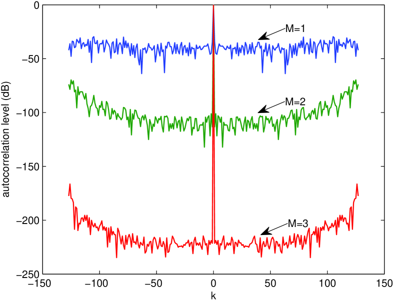
Figure 1: Autocorrelation levels of sequence sets with $N=128$ and $M=1,2,3$.

VII-B Approaching the Lower Bound of $\Psi$

As have been mentioned earlier, the criterion $\Psi$ defined in (5) is lower bounded by $N^{2}M(M-1)$. Then a natural question is whether we can achieve that bound. In this subsection, we apply the proposed MM-Corr and MM-WeCorr algorithms to minimize the criterion $\Psi$, i.e., solving problem (7), and compare the performance with the CAN algorithm [14].

In the experiment, we consider sequences sets with $M\in\{2,3,4\}$ sequences and each sequence of length $N\in\{256,1024\}$. For all algorithms, the initial sequence set was generated randomly as in the previous subsection, and the stopping criterion was set to be $\left|\Psi^{(l+1)}-\Psi^{(l)}\right|/\Psi^{(l)}\leq 10^{-8}$.

For each $(M,N)$ pair, the algorithms were repeated 10 times and the minimum and average values of $\Psi$ achieved by the three algorithms, together with the corresponding lower bound, are shown in Table I. The average running time of the three algorithms was also recorded and is provided in Table II. From Table I, we can see that all the three algorithms can get reasonably close to the lower bound of $\Psi$, which means the sequence sets generated by the algorithms are almost optimal for the $(M,N)$ pairs that have been considered. Another point we notice is that, for all $(M,N)$ pairs and all algorithms, the average values over 10 random trials are quite close to the minimum values, which implies that the three algorithms are not sensitive to the initial points. From Table II, we can see that for each $(M,N)$ pair, the MM-Corr algorithm is the fastest and the CAN algorithm is the slowest among the three algorithms. Since the per iteration computational complexity of MM-Corr and CAN is almost the same ($2M$ $2N$-point FFT (IFFT) operations), it implies that MM-Corr takes far fewer iterations to converge compared with CAN. Another observation is that for the same sequence length $N$, the cases with larger $M$ values take less time compared with the cases with smaller $M$ values, for example the running time of the algorithms for the pair $(M=4,N=256)$ is less than that for $(M=2,N=256)$. Since a larger $M$ value means higher per iteration computational complexity, the observation implies that when $M$ becomes larger, the algorithms need much fewer iterations to converge. It probably further implies that it is easier for a larger set of sequences to approach the lower bound than a smaller set of sequences.

Table I: The lower bound of $\Psi$ in (5) and the values achieved by different algorithms.

	CAN		MM-WeCorr		MM-Corr		Lower Bound
	minimum	average	minimum	average	minimum	average
$M=2,N=256$	131082	131089	131083	131093	131079	131093	131072
$M=3,N=256$	393220	393222	393217	393220	393219	393222	393216
$M=4,N=256$	786436	786439	786433	786436	786433	786436	786432
$M=2,N=1024$	2097336	2097394	2097426	2098298	2097335	2097453	2097152
$M=3,N=1024$	6291553	6291580	6291486	6291556	6291504	6291548	6291456
$M=4,N=1024$	12582992	12583019	12582937	12582989	12582939	12582992	12582912

Table II: The average running time (in seconds) of different algorithms over 10 random trials.

	CAN	MM-WeCorr	MM-Corr
$M=2,N=256$	9.3342	0.6765	0.2435
$M=3,N=256$	2.3461	0.3813	0.1000
$M=4,N=256$	1.3562	0.3822	0.0844
$M=2,N=1024$	33.8459	1.2011	0.6137
$M=3,N=1024$	8.0584	1.0797	0.2750
$M=4,N=1024$	4.9846	1.0298	0.2242

VII-C Sequence Set Design with Zero Correlation Zone

As can be seen from the previous subsection, it is impossible to design a set of sequences with all auto- and cross-correlation sidelobes very small. Since in some applications, it is enough to minimize the correlations only within a certain time lag interval, in this subsection we present an example of applying the proposed MM-WeCorr algorithm to design a set of sequences with low correlation sidelobes only at required lags and compare the performance with the WeCAN algorithm in [14]. The Matlab code of the WeCAN algorithm was downloaded from the website of the book [1].

Suppose we want to design a sequence set with $M=3$ sequences each of length $N=256$ and with low auto- and cross-correlations only at lags $k=51,\ldots,80$. To tackle the problem, we apply the MM-WeCorr and WeCAN algorithms from random initial sequence sets generated as in the previous subsections. For the MM-WeCorr algorithm, we choose the weights $\{w_{k}\}_{k=0}^{N-1}$ as follows:

$$w_{k}=\begin{cases}1,&k\in\{51,\dots,80\}\\ 0,&{\rm otherwise},\end{cases}$$ (94)

so that only the correlations at the required lags will be minimized. For both algorithms, we do not stop until the objective in (8) goes below $10^{-10}$ or after 10000 seconds. The evolution curves of the objective with respect to the running time are shown in Fig. 2. From the figure we can see that the proposed MM-WeCorr algorithm drives the objective to $10^{-10}$ within $1$ second, while the objective is still above $10^{2}$ after 10000 seconds for WeCAN. This is because the proposed MM-WeCorr algorithm requires about $3M^{2}+4M$ $2N$-point FFT’s per iteration, while each iteration of WeCAN requires $2MN$ computations of $2N$-point FFT’s and also $2N$ computations of the SVD of $M\times N$ matrices. The slower convergence of WeCAN may be another reason. Fig. 3 shows the auto- and cross-correlations (normalized by $N$) of the sequence sets generated by the two algorithms. We can see in Fig. 3 that the correlation sidelobes of the MM-WeCorr sequence set are suppressed to almost zero (about -175 dB) at the required lags, while that of the WeCAN sequence set is much higher. Another observation is that the cross-correlations at lag $k=0$ for the WeCAN sequence set are very low, although we did not try to suppress them. The reason is that in WeCAN, the weight at lag $0$ should be always positive and in fact large enough to ensure some weight matrix to be positive semidefinite. Thus the “0-lag” correlations are in fact emphasized the most in WeCAN. Note that in MM-WeCorr, the weight at lag $0$, i.e., $w_{0}$, can take any nonnegative value, thus it is more flexible to some extent.

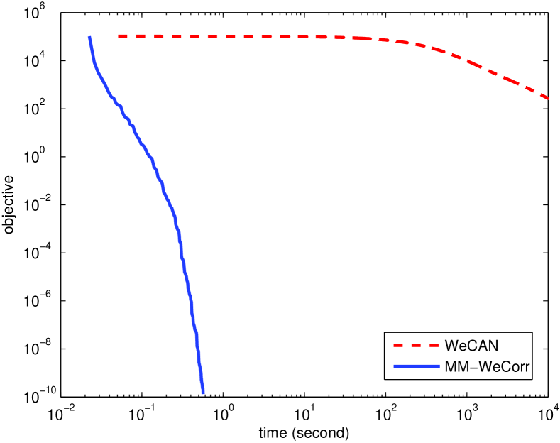
Figure 2: Evolution of the objective with respect to the running time (in seconds).

Figure 3: Auto- and cross-correlations of the 256-by-3 sequence sets generated by MM-WeCorr and WeCAN.

VIII Conclusion

In this paper, we have developed several efficient MM algorithms which can be used to design unimodular sequence sets with almost complementary autocorrelations or with both good auto- and cross-correlations. The proposed algorithms can be viewed as extensions of some single sequence design algorithms in the literature and share the same convergence properties, i.e., the convergence to a stationary point. In addition, all the algorithms can be implemented via FFT and thus are computationally very efficient. Numerical experiments show that the proposed CSS design algorithm can generate an almost complementary set of sequences as long as the cardinality of the set is not too small. In the case of sequence set design for both good auto- and cross-correlation properties, the proposed algorithms can get as close to the lower bound of the correlation criterion as the state-of-the-art method and are much faster. It has also been observed that the proposed weighted correlation minimization algorithm can produce sets of unimodular sequences with virtually zero auto- and cross-correlations at specified time lags.

Appendix A Proof of Lemma 5

Proof:

First, with Lemma 2, we have

$$\,\,\lambda_{{\rm max}}\left(\mathbf{R}-\mathbf{B}\circ\big{(}\mathbf{x}^{(l)}(\mathbf{x}^{(l)})^{H}\big{)}\right)$$ (95)

$$\leq \,\,\lambda_{{\rm max}}(\mathbf{R})-\lambda_{{\rm min}}\left(\mathbf{B}\circ\big{(}\mathbf{x}^{(l)}(\mathbf{x}^{(l)})^{H}\big{)}\right)$$

$$= \,\,\lambda_{{\rm max}}(\mathbf{R})-\lambda_{{\rm min}}\left(\mathbf{B}\right).$$

Then, according to Lemma 3, it is easy to see that

$$\lambda_{{\rm min}}\left(\mathbf{B}\right)=\begin{cases}\min\{M\lambda_{{\rm min}}(\mathbf{W}),0\},&M\geq 2\\ \lambda_{{\rm min}}(\mathbf{W}),&M=1,\end{cases}$$ (96)

and noticing the fact that $\mathbf{W}$ is symmetric Toeplitz, we know from Lemma 4 that

$$\lambda_{{\rm min}}(\mathbf{W})\geq\lambda_{W}.$$ (97)

Thus,

$$\lambda_{{\rm min}}\left(\mathbf{B}\right)\geq\lambda_{B}=\begin{cases}\min\left\{M\lambda_{W},0\right\},&M\geq 2\\ \lambda_{W},&M=1,\end{cases}$$ (98)

and we have

$$\lambda_{{\rm max}}\left(\mathbf{R}-\mathbf{B}\circ\big{(}\mathbf{x}^{(l)}(\mathbf{x}^{(l)})^{H}\big{)}\right)\leq\left\|\mathbf{R}\right\|-\lambda_{B},$$ (99)

where $\left\|\mathbf{R}\right\|$ can be any submultiplicative matrix norm of $\mathbf{R}$. ∎

Appendix B Proof of Lemma 6

Proof:

The $N\times N$ Toeplitz matrix $\mathbf{T}$ can be embedded in a circulant matrix $\mathbf{C}$ of dimension $2N\times 2N$ as follows:

$$\mathbf{C}=\left[\begin{array}[]{cc}\mathbf{T}&\mathbf{W}\\ \mathbf{W}&\mathbf{T}\end{array}\right],$$ (100)

where

$$\mathbf{W}=\begin{bmatrix}0&t_{1-N}&\cdots&t_{-1}\\ t_{N-1}&0&\ddots&\vdots\\ \vdots&\ddots&\ddots&t_{1-N}\\ t_{1}&\cdots&t_{N-1}&0\end{bmatrix}.$$ (101)

The circulant matrix $\mathbf{C}$ can be diagonalized by the FFT matrix [22], i.e.,

$$\mathbf{C}=\frac{1}{2N}\mathbf{F}^{H}{\rm Diag}(\mathbf{F}\mathbf{c})\mathbf{F},$$ (102)

where $\mathbf{c}$ is the first column of $\mathbf{C},$ i.e., $\mathbf{c}=[t_{0},t_{-1},\cdots,t_{1-N},0,t_{N-1},\cdots,t_{1}]^{T}.$ Since the matrix $\mathbf{T}$ is just the upper left $N\times N$ block of $\mathbf{C}$, we can easily obtain $\mathbf{T}=\frac{1}{2N}\mathbf{F}_{:,1:N}^{H}{\rm Diag}(\mathbf{F}\mathbf{c})\mathbf{F}_{:,1:N}$. ∎

Appendix C Proof of Lemma 7

Proof:

For any given $x_{0}\in[0,t)$, let us consider the quadratic function of the following form:

$$g(x|x_{0})=x_{0}^{4}+4x_{0}^{3}(x-x_{0})+a(x-x_{0})^{2},$$ (103)

where $a>0$. It is easy to check that $f(x_{0})=g(x_{0}|x_{0}).$ So to make $g(x|x_{0})$ be a majorization function of $f(x)$ at $x_{0}$ over the interval $[0,t]$, we need to further have $f(x)\leq g(x|x_{0})$ for all $x\in[0,t]$. Equivalently, we must have

$$a \geq\frac{x^{4}-x_{0}^{4}-4x_{0}^{3}(x-x_{0})}{(x-x_{0})^{2}}$$ (104)

$$=x^{2}+2x_{0}x+3x_{0}^{2}$$

for all $x\in[0,t]$. Let us define the function

$$A(x|x_{0})=x^{2}+2x_{0}x+3x_{0}^{2},$$ (105)

then condition (104) is equivalent to

$$a \geq\max_{x\in[0,t]}\,A(x|x_{0}).$$ (106)

Since the derivative of $A(x|x_{0})$, given by

$$A^{\prime}(x|x_{0})=2x+2x_{0},$$ (107)

is nonnegative for all $x\in[0,t],$ we know that $A(x|x_{0})$ is nondecreasing on the interval $[0,t]$ and the maximum is achieved at $x=t.$ Thus, condition (106) becomes

$$a \geq A(t|x_{0})$$ (108)

$$=t^{2}+2x_{0}t+3x_{0}^{2}.$$

Finally, by appropriately rearranging the terms of $g(x|x_{0})$ in (103), we can obtain the function in (73). The proof is complete. ∎

References

• [1] H. He, J. Li, and P. Stoica, Waveform Design for Active Sensing Systems: A Computational Approach.   Cambridge University Press, 2012.
• [2] N. Levanon and E. Mozeson, Radar Signals.   John Wiley & Sons, 2004.
• [3] P. Stoica, H. He, and J. Li, “New algorithms for designing unimodular sequences with good correlation properties,” IEEE Transactions on Signal Processing, vol. 57, no. 4, pp. 1415–1425, 2009.
• [4] J. Song, P. Babu, and D. P. Palomar, “Optimization methods for designing sequences with low autocorrelation sidelobes,” IEEE Transactions on Signal Processing, vol. 63, no. 15, pp. 3998–4009, Aug. 2015.
• [5] ——, “Sequence design to minimize the weighted integrated and peak sidelobe levels,” submitted to IEEE Transactions on Signal Processing, 2015. [Online]. Available: http://arxiv.org/abs/1506.04234
• [6] S. Searle, S. Howard, and B. Moran, “The use of complementary sets in MIMO radar,” in 2008 42nd Asilomar Conference on Signals, Systems and Computers, Oct. 2008, pp. 510–514.
• [7] N. Levanon, “Noncoherent radar pulse compression based on complementary sequences,” IEEE Transactions on Aerospace and Electronic Systems, vol. 45, no. 2, pp. 742–747, April 2009.
• [8] K. Schmidt, “Complementary sets, generalized Reed-Muller codes, and power control for OFDM,” IEEE Transactions on Information Theory, vol. 53, no. 2, pp. 808–814, Feb. 2007.
• [9] E. Garcia, J. Garcia, J. Urena, M. Perez, and D. Ruiz, “Multilevel complementary sets of sequences and their application in UWB,” in 2010 International Conference on Indoor Positioning and Indoor Navigation (IPIN), Sep. 2010, pp. 1–5.
• [10] S.-M. Tseng and M. Bell, “Asynchronous multicarrier DS-CDMA using mutually orthogonal complementary sets of sequences,” IEEE Transactions on Communications, vol. 48, no. 1, pp. 53–59, Jan. 2000.
• [11] P. Spasojevic and C. Georghiades, “Complementary sequences for ISI channel estimation,” IEEE Transactions on Information Theory, vol. 47, no. 3, pp. 1145–1152, Mar. 2001.
• [12] M. Soltanalian, M. M. Naghsh, and P. Stoica, “A fast algorithm for designing complementary sets of sequences,” Signal Processing, vol. 93, no. 7, pp. 2096–2102, 2013.
• [13] I. Oppermann and B. Vucetic, “Complex spreading sequences with a wide range of correlation properties,” IEEE Transactions on Communications, vol. 45, no. 3, pp. 365–375, Mar. 1997.
• [14] H. He, P. Stoica, and J. Li, “Designing unimodular sequence sets with good correlations–including an application to MIMO radar,” IEEE Transactions on Signal Processing, vol. 57, no. 11, pp. 4391–4405, Nov. 2009.
• [15] D. R. Hunter and K. Lange, “A tutorial on MM algorithms,” The American Statistician, vol. 58, no. 1, pp. 30–37, 2004.
• [16] P. Stoica and Y. Selen, “Cyclic minimizers, majorization techniques, and the expectation-maximization algorithm: a refresher,” IEEE Signal Processing Magazine, vol. 21, no. 1, pp. 112–114, Jan. 2004.
• [17] M. Razaviyayn, M. Hong, and Z.-Q. Luo, “A unified convergence analysis of block successive minimization methods for nonsmooth optimization,” SIAM Journal on Optimization, vol. 23, no. 2, pp. 1126–1153, 2013.
• [18] H. Roger and R. J. Charles, Topics in Matrix Analysis.   Cambridge University Press, 1994.
• [19] P. J. S. G. Ferreira, “Localization of the eigenvalues of Toeplitz matrices using additive decomposition, embedding in circulants, and the Fourier transform,” in Proceedings of the 10th IFAC Symposium on System Identification, Copenhagen, Denmark, Jul. 1994, pp. 271–276.
• [20] D. P. Bertsekas, A. Nedić, and A. E. Ozdaglar, Convex Analysis and Optimization.   Athena Scientific, 2003.
• [21] R. Varadhan and C. Roland, “Simple and globally convergent methods for accelerating the convergence of any EM algorithm,” Scandinavian Journal of Statistics, vol. 35, no. 2, pp. 335–353, 2008.
• [22] R. M. Gray, Toeplitz and Circulant Matrices: A review.   Now Publishers Inc, Jan. 2006, vol. 2, no. 3.