Exponential mixing for SPDEs driven by highly degenerate Lévy noises

Abstract.

By a coupling method, we prove that a family of stochastic partial differential equations (SPDEs) driven by highly degenerate pure jump Lévy noises are exponential mixing. These pure jump Lévy noises include $\alpha$-stable process with $\alpha\in(0,2)$.

1. Introduction

Let $\mathbb{H}$ be a Hilbert space with a complete orthonormal basis $\{e_{k}\}_{k\in\mathbb{N}}$. Let $A:\mathcal{D}(A)\subset\mathbb{H}\to\mathbb{H}$ be a self-adjoint operator such that

$$Ae_{n}=-\lambda_{n}e_{n},\ \ \ \ n\in\mathbb{N}$$

where $0<\lambda_{1}\leq\lambda_{2}\leq...$ and $\lim_{n\rightarrow\infty}\lambda_{n}=\infty$. We are concerned with the following stochastic PDEs:

(1.1) $${\rm d}X_{t}=[AX_{t}+F(X_{t})]{\rm d}t+{\rm d}L_{t}$$

where $F:\mathbb{H}\rightarrow\mathbb{H}$ is bounded and Lipschitz and $L_{t}$ is a $D$-dimensional pure jump Lévy process on the subspace ${\rm span}\{e_{1},...,e_{D}\}$ (see Assumption 1.1 below). Before giving the main theorem, let us first point out that the problem (1.1) is well-posed. By the same method as in [24, Sect. 5.1], we can show that for any initial data $x\in\mathbb{H}$, equation (1.1) has a unique mild solution $(X^{x}(t))_{t\geq 0}$ with Markov property as follows:

(1.2) $$X^{x}(t)=e^{At}x+\int_{0}^{t}e^{A(t-s)}F(X^{x}(s)){\rm d}s+\int_{0}^{t}e^{A(t-s)}{\rm d}L_{s}.$$

Moreover, $(X^{x}(t))_{t\geq 0}$ has a c$\grave{a}$dl$\grave{a}$g version in $\mathbb{H}$ since $L_{t}$ is finite dimension. Stochastic PDEs driven by non-degenerate Lévy noise have been intensively studied in the past decades, see [1, 3, 4, 7, 11, 15, 16, 21, 24] and the references therein.

Eq. (1.1) is a highly degenerate stochastic partial differential equations (SPDEs) with Lévy type noises. As $L_{t}$ is highly degenerate Wiener type or kick type noises, its ergodicity and related problems have been intensively studied recently, see [8, 9, 10, 19, 20] for Wiener type noises and [13, 12, 26, 18] for kick type noises. When $L_{t}$ is highly degenerate Lévy noises, to our knowledge, there seem no ergodicity results. One aim of our paper is to partly fill in this gap.

The third author of this paper studied in [29] a 2d degenerate SDE driven by 1d Lévy noises, as the dissipation in the direction not driven by noises is sufficiently strong, the stochastic system is exponentially mixing. This paper will prove the same result for highly degenerate SPDE (1.1), and adopt some notations and auxiliary lemmas in [29] for readers’ convenience. We shall use a similar approach as in [29] to proving exponential ergodicity, but we have to conquer some difficulties due to the infinite dimension (see Sections 2 and 3 below). Moreover, our new coupling construction is much more involved and the proof is simplified with a different strategy.

In section 2, we give an example similar to Example 2.9 in [22]. The latter example shows that a one dimensional SPDE driven by non-degenerate $\alpha$-stable noise with $\alpha\in(1,2)$ is exponential mixing, while the latter one in this paper indicates that as $\alpha$-stable noise is highly degenerate, the SPDE can be $d$-dimensional for all $d\geq 1$ and $\alpha$ can be in $(0,2)$. The two restrictions $d=1$ and $\alpha\in(1,2)$ in Example 2.9 of [22] are hard to be removed due to the limitation of the Harris’ approach to ergodicity (see also [5, 6] for some other examples). So, from these two examples, we can see that our coupling approach has big advantage for studying the ergodicity of stochastic Lévy type systems .

The structure of the paper is as follows. The remaining part of this section introduces the notations and gives the main theorem. Section 2 gives an example to which our main theorem is applicable and shows that Lévy type noises include $\alpha$-stable noise with $\alpha\in(0,2)$. We construct a coupling Markov process in the 3rd section and prove its properties which are important for estimating the stopping times in Section 4. In the last section, we prove the main theorem with a strategy given at the beginning.

1.1. Some preliminary of Lévy process ([2]) and the assumptions

Let $L_{t}$ be a D-dimensional Lévy process with Lévy measure $\nu$, denote

$$\Delta L_{t}=L_{t}-L_{t-}.$$

For any $K>0$, define

$$\Gamma_{K}:=\{y\in\mathbb{R}^{D}:|y|\geq K\},\quad\gamma_{K}:=\nu(\Gamma_{K}).$$

Note that $\gamma_{K}$ is a decreasing function of $K$ and $\gamma_{K}<\infty$ for any $K>0$.

For any $T>0$, define

(1.3) $$\tau:=\inf\{t>T:|\Delta L_{t}|\geq K\}.$$

Then $\tau$ is a stopping time with density

$$\gamma_{K}\exp\{-\gamma_{K}(t-T)\}1_{\{t>T\}}.$$

Define $\tau_{0}:=0$ and

$$\tau_{k}:=\inf\left\{t>\tau_{k-1}+T:|\Delta L(t)|\geq K\right\}\ \ \ {\rm for\ all\ }k\geq 1.$$

It is easy to see that $\{\tau_{k}\}_{k\geq 0}$ are a sequence of stopping times such that

(1.4) $$\{\tau_{k}-\tau_{k-1}\}_{k\geq 1}{\rm\ are\ independent\ and\ have\ the\ same\ density\ as}\ \tau.$$

Assumption 1.1.

We assume that

• $\sup_{0\leq t<\infty}\mathbb{E}\left|\int_{0}^{t}e^{A(t-s)}{\rm d}L_{s}\right|^{p}<\infty$ for $p\in(0,\alpha)$ with some $\alpha>0$.

• For some $K>0$, $\nu_{K}$ has a density $p_{K}$ such that for all $x_{1},x_{2}\in\mathbb{R}^{D}$,

  $$\int_{\mathbb{R}^{D}}|p_{K}(z-x_{1})-p_{K}(z-x_{2})|dz\leq\beta_{1}|x_{1}-x_{2}|^{\beta_{2}},$$

  where $\beta_{1},\beta_{2}>0$ are constants only depending on $K$.

• There exist some $M>0$ and some $\beta_{0}=\beta_{0}(K,M)\in(0,2)$ such that if $|x_{1}|+|x_{2}|\leq M$,

  $$\int_{\mathbb{R}^{D}}|p_{K}(z-x_{1})-p_{K}(z-x_{2})|dz\leq\beta_{0}.$$

• $\gamma_{K}\geq 2\beta_{2}\|F\|_{{\rm Lip}}$.

Remark 1.2.

The number “$2$”in “$\gamma_{K}\geq 2\beta_{2}\|F\|_{{\rm Lip}}$” of (A4) can be replaced by any number $c>1$. We choose the special “$2$” to make the computation in sequel more simple. The number $M$ will be chosen in Theorem 4.1.

1.2. Some notations for the further use

Denote by $B_{b}(\mathbb{H})$ the Banach space of bounded Borel-measurable functions $f:\mathbb{H}\rightarrow\mathbb{R}$ with the norm

$$\|f\|_{0}:=\sup_{x\in\mathbb{H}}|f(x)|.$$

Denote by $L_{b}(\mathbb{H})$ the Banach space of global Lipschitz bounded functions $f:\mathbb{H}\rightarrow\mathbb{R}$ with the norm

$$\|f\|_{1}:=\|f\|_{0}+\|f\|_{{\rm Lip}}.$$

where $\|f\|_{{\rm Lip}}:=\sup_{x\neq y}\frac{|f(x)-f(y)|}{\|x-y\|_{\mathbb{H}}}.$

Let $\mathcal{B}(\mathbb{H})$ be the Borel $\sigma$-algebra on $\mathbb{H}$ and let $\mathcal{P}(\mathbb{H})$ be the set of probability measures on $(\mathbb{H},\mathcal{B}(\mathbb{H}))$. Recall that the total variation distance between two measures $\mu_{1},\mu_{2}\in\mathcal{P}(\mathbb{H})$ is defined by

$$\|\mu_{1}-\mu_{2}\|_{\rm TV}:=\frac{1}{2}\sup_{\stackrel{{\scriptstyle f\in B_{b}(\mathbb{H})}}{{\|f\|_{0}=1}}}|\mu_{1}(f)-\mu_{2}(f)|=\sup_{\Gamma\in\mathcal{B}(\mathbb{H})}|\mu_{1}(\Gamma)-\mu_{2}(\Gamma)|.$$

Given a random variable $X$, we shall use

$$\mathcal{L}(X){\rm\ to\ denote\ the\ distribution\ of\ X.}$$

Let $\Pi$ be the orthogonal projection from $\mathbb{H}$ to the subspace ${\rm span}\{e_{1},...,e_{D}\}$. For any $x\in\mathbb{H}$, define

(1.5) $$x_{1}=\Pi x,\ \ \ \ x_{2}=(Id-\Pi)x.$$

For the further use, we denote

$$\mathbb{H}_{1}:={\rm span}\{e_{1},...,e_{D}\},\ \ \ \mathbb{H}_{2}:={\rm span}\{e_{D+1},e_{D+2},...,\}.$$

Then Eq. (1.1) can be written as

(1.6) $${\rm d}X_{1}(t)=[AX_{1}(t)+F_{1}(X(t))]{\rm d}t+{\rm d}L_{t},$$

(1.7) $${\rm d}X_{2}(t)=[AX_{2}(t)+F_{2}(X(t))]{\rm d}t.$$

Let us denote by $(P_{t})_{t\geq 0}$ the Markov semigroup associated with Eq.  (1.1), i.e.

$$P_{t}f(x):=\mathbb{E}\left[f(X^{x}(t))\right],\quad f\in B_{b}(\mathbb{H}),$$

and by $(P^{*}_{t})_{t\geq 0}$ the dual semigroup acting on $\mathcal{P}(\mathbb{H})$.

1.3. Main result

Our main result is the following ergodic theorem and it will be proven in the last section.

Theorem 1.3.

Under Assumption 1.1, if $D$ is sufficiently large, then the system (1.1) is ergodic and exponentially mixing under the weak topology of $\mathcal{P}(\mathbb{H})$. More precisely, there exists a unique invariant measure $\mu\in\mathcal{P}(\mathbb{H})$ so that for any $p\in(0,\alpha)$ and any measure $\tilde{\mu}\in\mathcal{P}(\mathbb{H})$ with finite $p^{\rm th}$ moment, we have

(1.8) $$\left|\int_{\mathbb{H}}f{\rm d}P^{*}_{t}\tilde{\mu}-\int_{\mathbb{H}}f{\rm d}\mu\right|\leq Ce^{-ct}\|f\|_{1}\left(1+\int_{\mathbb{H}}|x|^{p}\tilde{\mu}(dx)\right)\ \ \ \ \forall\ f\in L_{b}(\mathbb{H}),$$

where $C,c$ depend on $p,K,\|F\|_{{\rm Lip}},\|F\|_{0},\lambda_{1},\lambda_{D+1}$.

2. Examples and some preliminary estimates for the solution of Eq. (1.1)

2.1. Some concrete examples for Eq. (1.1)

We first claim that

Proposition 2.1.

$D$-dimensional rotationally symmetric $\alpha$-stable process $L_{t}$, with $0<\alpha<2$ and $D\in\mathbb{N}$, satisfies Assumption 1.1.

Before proving the proposition, we give an example below to which the assumptions of the paper applies, c.f. Example 2.9 in [22].

Example 2.2.

Consider the following stochastic semilinear equation on $\mathcal{D}=[0,\pi]^{d}$ with $d\geq 1$ and the Dirichlet boundary condition:

(2.1) $$\begin{cases}{\rm d}X(t,\xi)=[\Delta X(t,\xi)+F(X(t,\xi))]{\rm d}t+{\rm d}L_{t}(\xi),\\ X(0,\xi)=x(\xi),\\ X(t,\xi)=0,\ \ \xi\in\partial\mathcal{D},\end{cases}$$

where $F$ is bounded Lipschitz, $L_{t}$ is a $D$-dimensional rotationally symmetric $\alpha$-stable processes with $\alpha\in(0,2)$ to be further specified below.

It is well known that $\Delta$ with Dirichlet boundary condition has the following eigenfunctions

$$e_{k}(\xi)=\left(\frac{2}{\pi}\right)^{\frac{d}{2}}\sin(k_{1}\xi_{1})\cdots\sin(k_{d}\xi_{d}),\quad k\in\mathbb{N}^{d},\ \xi\in\mathcal{D}.$$

It is easy to see that $\Delta e_{k}=-|k|^{2}e_{k}$, i.e. $\gamma_{k}=|k|^{2}=k_{1}^{2}+\ldots+k_{d}^{2}$ for all $k\in\mathbb{N}^{d}$. We study the dynamics defined by (2.1) in the Hilbert space $\mathbb{H}=L^{2}(\mathcal{D})$ with orthonormal basis $\{e_{k}\}_{k\in\mathbb{N}^{d}}$.

$L_{t}$ is a $D$-dimensional symmetric $\alpha$-stable processes on the subspace ${\rm span}\{e_{1},...,e_{D}\}$. From our main result Theorem 1.3, for all $\alpha\in(0,2)$, as $D$ is sufficiently large, the stochastic system (2.1) converges to equilibrium measure exponentially fast.

Let us roughly compare our example with Example 2.9 of [22], which has the same form as Eq. (2.1) but with $d=1$ and $\alpha\in(1,2)$. The two restrictions $d=1$ and $\alpha\in(1,2)$ are hard to be removed due to the limitation of the Harris’ approach to ergodicity. To use Harris’ ergodicity theorem, one has to prove the strong Feller property which is true for Example 2.9 of [22] when $d=1$ and $L_{t}$ is non-degenerate $\alpha$-stable noises with $\alpha>1$. So, from these two examples, we can see the advantage of our coupling approach to the ergodicity.

Proof of Proposition 2.1.

Recall that $D$-dimensional rotationally symmetric $\alpha$-stable process $L_{t}$ has the following representation:

$$L_{t}=W_{S_{t}}$$

where $W_{t}=(W^{1}_{t},\ldots,W^{D}_{t})$ be a D-dimensional standard Brownian motion and $S_{t}$ is an $\alpha/2$-stable subordinator independent of $W_{t}$.

Let $\mathbb{E}^{\mathbb{S}},\mathbb{E}^{\mathbb{W}}$ denote the partial integrations with respect to $S$ and $W$ respectively, we have

(2.2) $$\begin{split}\mathbb{E}\left|\int_{0}^{t}e^{A(t-s)}{\rm d}L_{s}\right|^{p}&=\mathbb{E}^{\mathbb{S}}\left[\mathbb{E}^{\mathbb{W}}\left(\int_{0}^{t}e^{A(t-s)}{\rm d}W_{\ell_{s}}\right)^{p}\big{|}_{\ell.=S.}\right]\\ &\leq\mathbb{E}^{\mathbb{S}}\left[\left(\int_{0}^{t}\sum_{i=1}^{D}e^{-2\lambda_{i}(t-s)}{\rm d}\ell_{s}\right)^{p/2}\big{|}_{\ell.=S.}\right]\\ &=\mathbb{E}\left(\int_{0}^{t}\sum_{i=1}^{D}e^{-2\lambda_{i}(t-s)}{\rm d}S_{s}\right)^{p/2}\\ &\leq D^{p/2}\mathbb{E}\left(\int_{0}^{t}e^{-2\lambda_{1}(t-s)}{\rm d}S_{s}\right)^{p/2}.\\ \end{split}$$

Then,

$$\begin{split}&\mathbb{E}\left(\int_{0}^{t}e^{-2\lambda_{1}(t-s)}{\rm d}S_{s}\right)^{p/2}\leq\mathbb{E}\left(\sum_{k=0}^{[t]}\int_{k}^{k+1}e^{-2\lambda_{1}(t-s)}{\rm d}S_{s}\right)^{p/2}\\ &\leq\sum_{k=0}^{[t]}\mathbb{E}\left(\int_{k}^{k+1}e^{-2\lambda_{1}(t-s)}{\rm d}S_{s}\right)^{p/2}\leq\sum_{k=0}^{[t]}e^{-p\lambda_{1}(t-k-1)}\mathbb{E}\left(S_{k+1}-S_{k}\right)^{p/2}\\ &=\mathbb{E}S^{p/2}_{1}\sum_{k=0}^{[t]}e^{-p\lambda_{1}(t-k-1)}\leq\mathbb{E}S^{p/2}_{1}e^{2p\lambda_{1}}\sum_{k=0}^{\infty}e^{-pk\lambda_{1}}.\end{split}$$

Thus, (A1) is immediately verified from the above estimates.

Let us now verify that (A2) holds for all $K>0$ (this is obviously stronger than (A2) itself). For any $K>0$, the density of $\nu_{K}$ is

$$p_{K}(z)=\frac{C}{|z|^{D+\alpha}}1_{\{|z|\geq K\}},$$

where $C=C_{\alpha,D,K}$ depends on $\alpha,D,K$.

Without loss of generality, we assume $x_{1}=0$, $x_{2}=(x,0,\ldots,0)$ with $x\in\mathbb{R}$. Denote $f(x):=\int_{\mathbb{R}^{D}}|p_{K}(z)-p_{K}(z-x_{2})|dz$, note $f(0)=0$. We will show

(2.3) $$\sup_{|x|\leq K}|f^{\prime}(x)|\leq C_{K}.$$

On the other hand, as $|x|>K$, we have

$$f(x)\leq 2\leq\frac{2}{K}|x|=\frac{2}{K}|x_{2}|.$$

Combining the above two relations, we immediately get

(2.4) $$\int_{\mathbb{R}^{D}}|p_{K}(z)-p_{K}(z-x_{2})|dz\leq\left(C_{K}\vee\frac{2}{K}\right)|x_{2}|.$$

Hence, we verified that (A2) holds with $\beta_{1}=C_{K}\vee\frac{2}{K}$ and $\beta_{2}=1$.

Let now show (2.3). We first divide $\mathbb{R}^{D}$ into several parts (for instance, see Figure 1 when $D=1$),

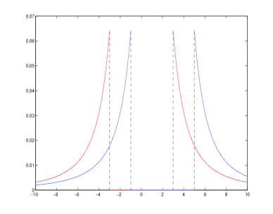
Figure 1. The red and blue lines are the functions of $\frac{1}{|z|^{1+\alpha}}1_{\{|z|\geq K\}}$ and $\frac{1}{|z-2|^{1+\alpha}}1_{\{|z-2|\geq K\}}$ with $\alpha=\frac{3}{2}$ and $K=3$ respectively.

$$f(x) = \int_{\mathbb{R}^{D}}\left|\frac{C}{|z|^{D+\alpha}}1_{|z|\geq K}-\frac{C}{|z-x_{2}|^{D+\alpha}}1_{|z-x_{2}|\geq K}\right|dz$$

$$= 2-4\int_{z_{1}\leq x/2,z^{2}_{1}+\cdots+z^{2}_{D}\geq K^{2}}\frac{C}{[(z_{1}-x)^{2}+z^{2}_{2}+\cdots+z^{2}_{D}]^{\frac{D+\alpha}{2}}}dz_{1}\cdots dz_{D}$$

$$\hat{=} 2-4g(x).$$

When $D=1$, we can easily get (2.3) holds. The proof of $D=2$ or $D\geq 3$ are almost the same, so we only study the case of $D\geq 3$ for convenience, using the transformation of spherical coordinates, i.e.

$$z_{1} = r\cos\theta_{1},$$

$$z_{2} = r\sin\theta_{1}\cos\theta_{2},$$

$$\ldots$$

$$z_{D-1} = r\sin\theta_{1}\sin\theta_{2}\cdots\cos\theta_{D-1},$$

$$z_{D} = r\sin\theta_{1}\sin\theta_{2}\cdots\sin\theta_{D-1},$$

where $\theta_{1},\ldots,\theta_{D-2}\in[0,\pi]$, $\theta_{D-1}\in[0,2\pi]$, $r\geq 0$. Then, we have

$$g(x) = \int_{r\cos\theta_{1}\leq x/2,r\geq K}\frac{Cr^{D-1}\sin^{D-2}\theta_{1}\sin^{D-3}\theta_{2}\cdots\sin\theta_{D-2}}{[(r\cos\theta_{1}-x)^{2}+r^{2}\sin^{2}\theta_{1}]^{\frac{D+\alpha}{2}}}d\theta_{1}\cdots d\theta_{D-1}dr$$

$$= C_{\alpha,D}\int_{K}^{\infty}\int^{\pi}_{arc\cos\frac{x}{2r}}\frac{r^{D-1}\sin^{D-2}\theta_{1}}{\left[(r\cos\theta_{1}-x)^{2}+r^{2}\sin^{2}\theta_{1}\right]^{\frac{D+\alpha}{2}}}drd\theta_{1}.$$

Take the derivative with respect to $x$, we get

$$g^{\prime}(x)=\!\!\!\!\!\!\!\!\!\! C_{\alpha,D}\int_{K}^{\infty}\frac{\left(1-\frac{x^{2}}{4r^{2}}\right)^{\frac{D-2}{2}}}{r^{\alpha+1}\sqrt{4r^{2}-x^{2}}}dr$$

$$+C_{\alpha,D}\int_{K}^{\infty}\int^{\pi}_{arc\cos\frac{x}{2r}}\frac{r^{D-1}\sin^{D-2}\theta_{1}(r\cos\theta_{1}-x)}{\left[(r\cos\theta_{1}-x)^{2}+r^{2}\sin^{2}\theta_{1}\right]^{\frac{D+\alpha}{2}+1}}drd\theta_{1}.$$

Then, it is easy to see that

$$\sup_{|x|\leq K}|g^{\prime}(x)|<C_{K},\quad\text{as}\quad|x|\leq K.$$

Hence, (2.3) holds.

Since the supports of the functions $p_{K}(z-x_{1})$ and $p_{K}(z-x_{2})$ have overlaps, it holds that

$$\begin{split}\phi(x_{1},x_{2}):&=\int_{\mathbb{R}^{D}}|p_{K}(z-x_{1})-p_{K}(z-x_{2})|dz\\ &<\int_{\mathbb{R}^{D}}p_{K}(z-x_{1})dz+\int_{\mathbb{R}^{D}}p_{K}(z-x_{2})dz=2.\end{split}$$

Since $\phi$ is a continuous function, for all $M>0$ there exists some $\beta_{0}\in(0,2)$ depending on $M$ and $K$ such that (A3) holds.

Since $L_{t}$ is $\alpha$-stable noise, $\gamma_{K}\rightarrow\infty$ as $K\downarrow 0$. Therefore, (A4) is clearly true. ∎

2.2. Some easy estimates about the solution

In this subsection, we prove some easy estimates about the solution $X(t)$ of Eq. (1.1), which will play an essential role for estimating some stopping times in the sections later.

Lemma 2.3.

The following statements hold:

1. For $x,y\in\mathbb{H}$, $p\in(0,\alpha)$, we have

   $$\mathbb{E}\|X^{x}(t)\|_{\mathbb{H}}^{p}\leq(3^{p-1}\vee 1)e^{-\lambda_{1}pt}\|x\|_{\mathbb{H}}^{p}+C\ \ \ \ \forall\ t\geq 0,$$

   $$\mathbb{E}\|X^{x}(t)-X^{y}(t)\|_{\mathbb{H}}^{p}\leq(2^{p-1}\vee 1)e^{-\lambda_{1}pt}\|x-y\|_{\mathbb{H}}^{p}+C\ \ \ \ \forall\ t\geq 0,$$

   where $a\vee b:=\max\{a,b\}$ for $a,b\in\mathbb{R}$ and $C$ depends on $p,\lambda_{1},\|F\|_{0}$.

2. For $x,y\in\mathbb{H}$, we have

   $$\|X^{x}(t)-X^{y}(t)\|_{\mathbb{H}}\leq e^{t\|F\|_{\rm Lip}}\|x-y\|_{\mathbb{H}},$$

   $$\|X^{x}_{2}(t)-X^{y}_{2}(t)\|_{\mathbb{H}}\leq\left(e^{-\lambda_{D+1}t}+\frac{\|F\|_{\rm Lip}}{\lambda_{D+1}+\|F\|_{\rm Lip}}\ e^{t\|F\|_{\rm Lip}}\right)\|x-y\|_{\mathbb{H}},$$

   for all $t\geq 0$.

Proof.

Denote

$$Z_{A}(t):=\int_{0}^{t}e^{A(t-s)}{\rm d}L_{s},$$

it is easy to see that $Z_{A}(t)$ is a D-dimensional stochastic process and

$$|Z_{A}(t)|=\|Z_{A}(t)\|_{\mathbb{H}}.$$

By (1.2) we have

$$\begin{split}\left\|X^{x}(t)\right\|_{\mathbb{H}}&\leq\left\|e^{At}x\right\|_{\mathbb{H}}+\left\|\int_{0}^{t}e^{A(t-s)}F(X^{x}(s)){\rm d}s\right\|_{\mathbb{H}}+\left|Z_{A}(t)\right|\\ &\leq e^{-\lambda_{1}t}\|x\|_{\mathbb{H}}+\int_{0}^{t}e^{-\lambda_{1}(t-s)}{\rm d}s\|F\|_{0}+\left|Z_{A}(t)\right|,\end{split}$$

and

$$\begin{split}\left\|X^{x}(t)-X^{y}(t)\right\|_{\mathbb{H}}&\leq\left\|e^{At}(x-y)\right\|_{\mathbb{H}}+\left\|\int_{0}^{t}e^{A(t-s)}[F(X^{x}(s))-F(X^{y}(s))]{\rm d}s\right\|_{\mathbb{H}}\\ &\leq e^{-\lambda_{1}t}\|x-y\|_{\mathbb{H}}+2\int_{0}^{t}e^{-\lambda_{1}(t-s)}{\rm d}s\|F\|_{0}.\end{split}$$

The first statement follows from the above inequality and (A1) of Assumption 1.1.

Let us now prove the second statement. It is easy to have

(2.5) $$X^{x}(t)-X^{y}(t)=e^{At}(x-y)+\int_{0}^{t}e^{A(t-s)}\left[F(X^{x}(s))-F(X^{y}(s))\right]{\rm d}s,$$

which implies

$$\|X^{x}(t)-X^{y}(t)\|_{\mathbb{H}}\leq\|x-y\|_{\mathbb{H}}+\int_{0}^{t}\|F\|_{\rm Lip}\|X^{x}(s)-X^{y}(s)\|_{\mathbb{H}}{\rm d}s.$$

From this we immediately get the first inequality by Gronwall’s inequality. It follows from (2.5) and the first inequality that

$$\begin{split}\|X^{x}_{2}(t)-X^{y}_{2}(t)\|_{\mathbb{H}}&\leq\|e^{At}(x_{2}-y_{2})\|_{\mathbb{H}}+\int_{0}^{t}\|e^{-A(t-s)}F_{2}(X^{x}(s))-F_{2}(X^{y}(s))\|_{\mathbb{H}}ds\\ &\leq e^{-\lambda_{D+1}t}\|x-y\|_{\mathbb{H}}+\int_{0}^{t}e^{-\lambda_{D+1}(t-s)}\|F\|_{\rm Lip}\|X^{x}(s))-X^{y}(s)\|_{\mathbb{H}}ds\\ &\leq e^{-\lambda_{D+1}t}\|x-y\|_{\mathbb{H}}+\int_{0}^{t}e^{-\lambda_{D+1}(t-s)}\|F\|_{\rm Lip}\ e^{s\|F\|_{\rm Lip}}\|x-y\|_{\mathbb{H}}ds.\end{split}$$

This immediately implies the second inequality. ∎

3. Construction of the coupling

In this section, let us first construct a coupling Markov process which will play an essential role for proving our ergodicity result, and then prove a preliminary estimate about this coupling.

3.1. Construction of the coupling

Lemma 3.1.

Let $X^{x}(t)$ and $X^{y}(t)$ be the solutions to the equation (1.1) for any given $x$ and $y$ respectively. Let $\tau$ be the stopping time defined by (1.3). Then, we have a probability space $(\tilde{\Omega},\tilde{\mathcal{F}},\tilde{\mathbb{P}})$, not depending on $x$ and $y$, on which there exist a random time $\tilde{\tau}$ and a coupling Markov process $S^{x,y}(t)=(S^{x}(t),S^{y}(t))_{0\leq t\leq\tau}$ on $(\tilde{\Omega},\tilde{\mathcal{F}},\tilde{\mathbb{P}})$ such that

• $\tilde{\tau}$, not depending on $x$ and $y$, has the same distribution as $\tau$;

• $\mathcal{L}((S^{x}(t))_{0\leq t\leq\tilde{\tau}})=\mathcal{L}((X^{x}(t))_{0\leq t\leq\tau})$ and $\mathcal{L}((S^{y}(t))_{0\leq t\leq\tilde{\tau}})=\mathcal{L}((X^{y}(t))_{0\leq t\leq\tau})$;

• the following equality holds:

  $$\tilde{\mathbb{P}}\bigg{(}S_{1}^{x}(\tilde{\tau})\neq S_{1}^{y}(\tilde{\tau})\big{|}S_{1}^{x}(\tilde{\tau}-),S_{1}^{y}(\tilde{\tau}-)\bigg{)}=\frac{1}{2}\int_{\mathbb{R}^{D}}|p_{K}(z-\hat{x}_{1})-p_{K}(z-\hat{y}_{1})|dz,$$

  where $\hat{x}_{1}=S_{1}^{x}(\tilde{\tau}-)$ and $\hat{y}_{1}=S_{1}^{y}(\tilde{\tau}-)$, and $S_{1}^{x}(\tilde{\tau}-)$ and $S_{1}^{y}(\tilde{\tau}-)$ are defined by the practice (1.5).

Proof.

Take a copy $(\tilde{\Omega}_{1},\tilde{\mathcal{F}_{1}},\tilde{\mathbb{P}}_{1})$ of $(\Omega,\mathcal{F},\mathbb{P})$ and consider the following SPDEs on $(\tilde{\Omega}_{1},\tilde{\mathcal{F}}_{1},\tilde{\mathbb{P}}_{1})$:

(3.1) $$\begin{cases}{\rm d}X(t)=[AX(t)+F(X(t))]{\rm d}t+{\rm d}\tilde{L}_{t},\\ X(0)=x,\end{cases}$$

and

(3.2) $$\begin{cases}{\rm d}X(t)=[AX(t)+F(X(t))]{\rm d}t+{\rm d}\tilde{L}_{t},\\ X(0)=y,\end{cases}$$

where $(\tilde{L}_{t})_{t\geq 0}$ has the same distribution as $(L_{t})_{t\geq 0}$.

Define

(3.3) $$\tilde{\tau}=\inf\{t\geq T:|\Delta\tilde{L}_{t}|\geq K\},$$

it is easy to see that $\tilde{\tau}$ has the same distribution as $\tau$. At the time $\tilde{\tau}$, there is a jump $\tilde{\eta}$ which is independent of $\tilde{\tau}$ and the processes $(X^{x}(t))_{0\leq t<\tilde{\tau}}$ and $(X^{y}(t))_{0\leq t<\tilde{\tau}}$. We have

$$X^{x}(\tilde{\tau})=X^{x}(\tilde{\tau}-)+\tilde{\eta},\ \ X^{y}(\tilde{\tau})=X^{y}(\tilde{\tau}-)+\tilde{\eta}.$$

Note that $\tilde{\eta}$ is a random variable valued on ${\rm span}\{e_{1},...,e_{D}\}$, then

$$\begin{split}&X^{x}_{1}(\tilde{\tau})=X^{x}_{1}(\tilde{\tau}-)+\tilde{\eta},\ \ X^{y}_{1}(\tilde{\tau})=X^{y}_{1}(\tilde{\tau}-)+\tilde{\eta};\\ &X^{x}_{2}(\tilde{\tau})=X^{x}_{2}(\tilde{\tau}-),\ \ \ \ \ \ \ \ X^{y}_{2}(\tilde{\tau})=X^{y}_{2}(\tilde{\tau}-).\\ \end{split}$$

where $X_{1}$ and $X_{2}$ is defined according to the practice in (1.5). For notational simplicity, write

(3.4) $$\begin{split}&\hat{x}_{1}:=X^{x}_{1}(\tilde{\tau}-),\ \ \hat{y}_{1}:=X^{y}_{1}(\tilde{\tau}-);\\ &\hat{x}_{2}:=X^{x}_{2}(\tilde{\tau}-),\ \ \hat{y}_{2}:=X^{y}_{2}(\tilde{\tau}-).\end{split}$$

Note that $\hat{x}_{1},\hat{x}_{2},\hat{y}_{1},\hat{y}_{2}$ above are all random variables on $(\tilde{\Omega}_{1},\tilde{\mathcal{F}_{1}},\tilde{\mathbb{P}}_{1})$.

Now consider the conditional probabilities $\mathcal{L}(X^{x}_{1}(\tilde{\tau})|\hat{x}_{1})$ and $\mathcal{L}(X^{y}_{1}(\tilde{\tau})|\hat{y}_{1})$, it is easy to see that these two probabilities respectively have the following densities:

$$p_{K}(z-\hat{x}_{1})\ \ \ \ \ {\rm and}\ \ \ \ p_{K}(z-\hat{y}_{1}).$$

By Theorem 4.2 of [13], there exists a probability space $(\tilde{\Omega}_{2},\tilde{\mathcal{F}}_{2},\tilde{\mathbb{P}}_{2})$ such that for any pair $(u,v)\in\mathbb{R}^{D}\times\mathbb{R}^{D}$, there exists a pair of random variables

$$\xi(u,v,\tilde{\omega}_{2})=(\xi^{x}(u,v,\tilde{\omega}_{2}),\xi^{y}(u,v,\tilde{\omega}_{2}))$$

satisfying the following properties:

• $\xi(u,v)$ is a maximal coupling of $p_{K}(z-u)$ and $p_{K}(z-v)$,

• the map $\xi(u,v,\tilde{\omega}_{2}):\mathbb{R}^{D}\times\mathbb{R}^{D}\times\tilde{\Omega}_{2}\rightarrow\mathbb{R}^{D}\times\mathbb{R}^{D}$ is measurable.

Take

$$(\tilde{\Omega},\tilde{\mathcal{F}},\tilde{\mathbb{P}})=(\tilde{\Omega}_{1},\tilde{\mathcal{F}}_{1},\tilde{\mathbb{P}}_{1})\times(\tilde{\Omega}_{2},\tilde{\mathcal{F}}_{2},\tilde{\mathbb{P}}_{2}),$$

from the procedure above, $\xi(\hat{x}_{1},\hat{y}_{1},\tilde{\omega}_{2})$ is a maximal coupling for the conditional probability $\mathcal{L}(X^{x}_{1}(\tilde{\tau})|\hat{x}_{1})$ and $\mathcal{L}(X^{y}_{1}(\tilde{\tau})|\hat{y}_{1})$. By the property of the maximal coupling,

(3.5) $$\tilde{\mathbb{P}}\left(\xi^{x}(\hat{x}_{1},\hat{y}_{1})\neq\xi^{y}(\hat{x}_{1},\hat{y}_{1})|\hat{x}_{1},\hat{y}_{1}\right)=\frac{1}{2}\int_{\mathbb{R}^{D}}|p_{K}(z-\hat{x}_{1})-p_{K}(z-\hat{y}_{1})|{\rm d}z.$$

On $(\tilde{\Omega},\tilde{\mathcal{F}},\tilde{\mathbb{P}})$, for every $\tilde{\omega}\in\tilde{\Omega}$ define

(3.6) $$\begin{split}&S^{x,y}(t,\tilde{\omega})=(X^{x}(t,\tilde{\omega}_{1}),X^{y}(t,\tilde{\omega}_{1})),\ \ \ \ 0\leq t<\tilde{\tau}(\tilde{\omega}_{1}),\\ &S^{x,y}(\tilde{\tau}(\tilde{\omega}_{1}),\tilde{\omega})=(\xi^{x}(\hat{x}_{1},\hat{y}_{1})+\hat{x}_{2},\xi^{y}(\hat{x}_{1},\hat{y}_{1})+\hat{y}_{2}),\end{split}$$

where

$$\xi^{x}(\hat{x}_{1},\hat{y}_{1})=\xi^{x}\big{(}\hat{x}_{1}(\tilde{\omega}_{1}),\hat{y}_{1}(\tilde{\omega}_{1}),\tilde{\omega}_{2}\big{)},$$

$$\xi^{y}(\hat{x}_{1},\hat{y}_{1})=\xi^{y}\big{(}\hat{x}_{1}(\tilde{\omega}_{1}),\hat{y}_{1}(\tilde{\omega}_{1}),\tilde{\omega}_{2}\big{)},$$

and $\hat{x}_{1},\hat{y}_{1},\hat{x}_{2},\hat{y}_{2}$ are defined in (3.4). (3) follows (3.5) immediately.

It remains to show (2). From the above construction, it is clear that $(S^{x}(t))_{0\leq t<\tilde{\tau}}$ and $(X^{x}(t))_{0\leq t<\tau}$ have the same distributions. Since $X^{x}(\tau)=X^{x}(\tau-)+\eta$ with $\eta$ being independent of $(X^{x}(t))_{0\leq t<\tau}$, given $X^{x}(\tau-)$, $X^{x}(\tau)$ is independent of $(X^{x}(t))_{0\leq t<\tau}$ and has probability densities $p_{K}(z-X_{1}^{x}(\tau-))$ in the subspace $\mathbb{H}_{1}$ and $\delta_{X_{2}^{x}(\tau-)}$ in the subspace $\mathbb{H}_{2}$. On the other hand, from the above coupling construction, $\mathcal{L}(S^{x}(\tilde{\tau})|S^{x,y}(\tilde{\tau}-))$ has probability densities $p_{K}(z-S_{1}^{x}(\tau-))$ in the subspace $\mathbb{H}_{1}$ and $\delta_{S_{2}^{x}(\tau-)}$ in the subspace $\mathbb{H}_{2}$. Integrating over $S^{y}(\tilde{\tau}-)$, we obtain that $\mathcal{L}(S^{x}(\tilde{\tau})|S^{x}(\tilde{\tau}-))$ has probability densities $p_{K}(z-S_{1}^{x}(\tau-))$ in the subspace $\mathbb{H}_{1}$ and $\delta_{S_{2}^{x}(\tau-)}$ in the subspace $\mathbb{H}_{2}$. This further implies that given $S^{x}(\tilde{\tau}-)$, $\tilde{\eta}:=S^{x}(\tilde{\tau})-S^{x}(\tilde{\tau}-)$ has a probability density $p_{K}(z)$ in the subspace $\mathbb{H}_{1}$ and $\delta_{0}$ in the subspace $\mathbb{H}_{2}$, it is clearly independent of $S^{x}(\tilde{\tau}-)$. Hence, $(X^{x}(t))_{0\leq t\leq\tau}$ and $(S^{x}(t))_{0\leq t\leq\tilde{\tau}}$ have the same distributions. By the same argument as above, we get that $(X^{y}(t))_{0\leq t\leq\tilde{\tau}}$ and $(S^{y}(t))_{0\leq t\leq\tilde{\tau}}$ have the same distributions. ∎

Lemma 3.2.

Let $X^{x}(t)$ and $X^{y}(t)$ be the solution to the equation (1.1) for any give $x\in\mathbb{H}$ and $y\in\mathbb{H}$ respectively. Then, there exists a probability space $(\bar{\Omega},\bar{\mathcal{F}},\bar{\mathbb{P}})$ on which

• there exists a Markov process $S^{x,y}(t)=(S^{x}(t),S^{y}(t))$ such that $S^{x}(t)$ and $S^{y}(t)$ have the same distributions as those of $X^{x}(t)$ and $X^{y}(t)$ respectively;

• there exists a stopping times sequences $(\tilde{\tau}_{k})_{k\geq 0}$ which has the same distribution as $(\tau_{k})_{k\geq 0}$;

• the following equality holds: for all $k\geq 1$,

  $$\bar{\mathbb{P}}\bigg{(}S_{1}^{x}(\tilde{\tau}_{k})\neq S_{1}^{y}(\tilde{\tau}_{k})\big{|}S_{1}^{x}(\tilde{\tau}_{k}-),S_{1}^{y}(\tilde{\tau}_{k}-)\bigg{)}=\frac{1}{2}\int_{\mathbb{R}^{D}}|p_{K}(z-z_{1})-p_{K}(z-z_{2})|dz,$$

  where $z_{1}=S_{1}^{x}(\tilde{\tau}_{k}-)$ and $z_{2}=S_{1}^{y}(\tilde{\tau}_{k}-)$.

Proof.

We shall prove the lemma by recursively applying Lemma 3.1. For the further use, recall the notations in Lemma 3.1 and denote $\tilde{\tau}_{0}:=0$, $\Delta\tilde{\tau}_{1}:=\tilde{\tau}$, $\tilde{\tau}_{1}:=\tilde{\tau}_{0}+\Delta\tilde{\tau}_{1}$ and $(\tilde{\Omega}^{1},\tilde{\mathcal{F}}^{1},\tilde{\mathbb{P}}^{1}):=(\tilde{\Omega},\tilde{\mathcal{F}},\tilde{\mathbb{P}})$.

Now taking $S^{x}(\tilde{\tau}_{1})$ and $S^{y}(\tilde{\tau}_{1})$ as initial data, by Lemma 3.1 we have a probability space $(\tilde{\Omega}^{(2)},\tilde{\mathcal{F}}^{(2)},\tilde{\mathbb{P}}^{(2)})$, a copy of $(\tilde{\Omega},\tilde{\mathcal{F}},\tilde{\mathbb{P}})$ in Lemma 3.1, on which there exists a stopping time $\Delta\tilde{\tau}_{2}$ and a Markov process $(S^{S^{x}(\tilde{\tau}_{1}),S^{y}(\tilde{\tau}_{1})}(t))_{0\leq t\leq\Delta\tilde{\tau}_{2}}$ with the properties (1)-(3).

Denote $(\tilde{\Omega}^{2},\tilde{\mathcal{F}}^{2},\tilde{\mathbb{P}}^{2})=(\tilde{\Omega}^{1},\tilde{\mathcal{F}}^{1},\tilde{\mathbb{P}}^{1})\times(\tilde{\Omega}^{(2)},\tilde{\mathcal{F}}^{(2)},\tilde{\mathbb{P}}^{(2)})$ and $\tilde{\tau}_{2}=\tilde{\tau}_{1}+\Delta\tilde{\tau}_{2}$, on this new space, for every $\tilde{\omega}=(\tilde{\omega}_{1},\tilde{\omega}_{2})\in(\tilde{\Omega}^{2},\tilde{\mathcal{F}}^{2},\tilde{\mathbb{P}}^{2})$ define

$$S^{x,y}(t,\tilde{\omega})=S^{x,y}(t,\tilde{\omega}_{1}),\ \ \ \ t\in[0,\tilde{\tau}_{1}(\tilde{\omega}_{1})],$$

$$S^{x,y}(t,\tilde{\omega})=S^{S^{x}(\tilde{\tau}_{1}(\tilde{\omega}_{1})),S^{y}(\tilde{\tau}_{1}(\tilde{\omega}_{1}))}(t-\tilde{\tau}_{1}(\omega_{1}),\tilde{\omega}_{2}),\ \ \ \ t\in[\tilde{\tau}_{1}(\tilde{\omega}_{1}),\tilde{\tau}_{2}(\tilde{\omega}_{2})].$$

It is clear that $\tilde{\tau}_{2}-\tilde{\tau}_{1}$ has the same distribution as $\tau$ and is independent of $\tilde{\tau}_{1}$ and that $\tilde{\tau}_{2}$ has the same distribution as $\tau_{2}$. We further claim that $(S^{x}(t))_{0\leq t\leq\tilde{\tau}_{2}}$ and $(S^{y}(t))_{0\leq t\leq\tilde{\tau}_{2}}$ have the same distributions as those of $(X^{x}(t))_{0\leq t\leq\tau_{2}}$ and $(X^{y}(t))_{0\leq t\leq\tau_{2}}$ respectively. Indeed, if $X^{x}(\tau_{1})=S^{x}(\tilde{\tau}_{1})=\hat{x}$ and $X^{y}(\tau_{1})=S^{y}(\tilde{\tau}_{1})=\hat{y}$ with $\hat{x},\hat{y}\in\mathbb{H}$, by (2) of Lemma 3.1, we have

$$\mathcal{L}((S^{x}(t))_{\tilde{\tau}_{1}\leq t\leq\tilde{\tau}_{2}}|S^{x}(\tilde{\tau}_{1})=\hat{x})=\mathcal{L}((X^{x}(t))_{\tau_{1}\leq t\leq\tau_{2}}|X^{x}(\tau_{1})=\hat{x}).$$

From Lemma 3.1, $\mathcal{L}(S^{x}(\tilde{\tau}_{1}))=\mathcal{L}(X^{x}(\tau_{1}))$. Hence, by Markov property, we have

$$\mathcal{L}((S^{x}(t))_{0\leq t\leq\tilde{\tau}_{2}})=\mathcal{L}((X^{x}(t))_{0\leq t\leq\tau_{2}}).$$

Similarly,

$$\mathcal{L}((S^{y}(t))_{0\leq t\leq\tilde{\tau}_{2}})=\mathcal{L}((X^{y}(t))_{0\leq t\leq\tau_{2}}).$$

By (3) of Lemma 3.1, the third property with $k=2$ in the lemma clearly holds.

Applying the same argument as above inductively, we have:

• a sequence of probability spaces $(\tilde{\Omega}^{1},\tilde{\mathcal{F}}^{1},\tilde{\mathbb{P}}^{1}),(\tilde{\Omega}^{2},\tilde{\mathcal{F}}^{2},\tilde{\mathbb{P}}^{2}),...,(\tilde{\Omega}^{k},\tilde{\mathcal{F}}^{k},\tilde{\mathbb{P}}^{k}),...$ with $(\tilde{\Omega}^{k},\tilde{\mathcal{F}}^{k},\tilde{\mathbb{P}}^{k})=(\tilde{\Omega},\tilde{\mathcal{F}},\tilde{\mathbb{P}})\times...\times(\tilde{\Omega},\tilde{\mathcal{F}},\tilde{\mathbb{P}})$ being the $k$-tuple direct product of $(\tilde{\Omega},\tilde{\mathcal{F}},\tilde{\mathbb{P}})$ and $(\bar{\Omega},\bar{\mathcal{F}},\bar{\mathbb{P}})=(\tilde{\Omega}^{\infty},\tilde{\mathcal{F}}^{\infty},\tilde{\mathbb{P}}^{\infty})$;

• a sequence of stopping times $(\tilde{\tau}_{k})_{k\geq 1}$ such that $\tilde{\tau}_{k}$ is located in $(\tilde{\Omega}^{k},\tilde{\mathcal{F}}^{k},\tilde{\mathbb{P}}^{k})$ for each $k\geq 1$ and $(\tilde{\tau}_{k}-\tilde{\tau}_{k-1})_{k\geq 1}$ is i.i.d. with the same distribution as $\tau$;

• a sequence of coupling Markov processes $((S^{x,y}(t))_{0\leq t\leq\tilde{\tau}_{k}})_{k\geq 1}$ such that $(S^{x,y}(t))_{0\leq t\leq\tilde{\tau}_{k}}$ is located in $(\tilde{\Omega}^{k},\tilde{\mathcal{F}}^{k},\tilde{\mathbb{P}}^{k})$ and $\mathcal{L}((S^{x}(t))_{0\leq t\leq\tilde{\tau}_{k}})=\mathcal{L}((X^{x}(t))_{0\leq t\leq\tau_{k}})$ and $\mathcal{L}((S^{y}(t))_{0\leq t\leq\tilde{\tau}_{k}})=\mathcal{L}((X^{y}(t))_{0\leq t\leq\tau_{k}})$ for all $k\geq 1$. Moreover, (3) in the lemma holds.

It is clear from (ii) that $\lim_{k\rightarrow\infty}\tau_{k}=\infty$ a.s. and $\lim_{k\rightarrow\infty}\tilde{\tau}_{k}=\infty$ a.s., this, together with (iii), immediately implies (1) in the lemma. ∎

3.2. Some estimates of the coupling chain $(S^{x,y}(\tilde{\tau}_{k}))_{k\geq 0}$

Recall that $(S^{x,y}(\tilde{\tau}_{k}))_{k\geq 0}$ is a Markov chain on the probability space $(\bar{\Omega},\bar{\mathcal{F}},\bar{\mathbb{P}})$. Note that $(\bar{\Omega},\bar{\mathcal{F}},\bar{\mathbb{P}})$ is not necessarily the same as $(\Omega,{\mathcal{F}},{\mathbb{P}})$ on which $(X^{x}(t))_{t\geq 0}$ and $(X^{y}(t))_{t\geq 0}$ is located. Without loss of generality, we assume that

(3.7) $$(\Omega,{\mathcal{F}},{\mathbb{P}})=(\bar{\Omega},\bar{\mathcal{F}},\bar{\mathbb{P}}).$$

Otherwise we can introduce the product space $(\bar{\Omega}\times\Omega,\bar{\mathcal{F}}\times\mathcal{F},\bar{\mathbb{P}}\times\mathbb{P})$ and consider $(S^{x,y}(k))_{k\geq 0}$, $(X^{x}(t))_{t\geq 0}$ and $(X^{y}(t))_{t\geq 0}$ all together on this new space. However, this will make the notations unnecessarily complicated, for instance, we have to always use $\bar{\mathbb{P}}\times\mathbb{P}$.

Proposition 3.3.

Let $\{\tilde{\tau}_{k}\}_{k\geq 0}$ be the stopping times sequence in Lemma 3.2 and let

(3.8) $$\delta_{k}:=e^{-\lambda_{D+1}(\tilde{\tau}_{k+1}-\tilde{\tau}_{k})}+\frac{\|F\|_{\rm Lip}e^{(\tilde{\tau}_{k+1}-\tilde{\tau}_{k})\|F\|_{\rm Lip}}}{\lambda_{D+1}+\|F\|_{\rm Lip}}.$$

For all $x,y\in\mathbb{H}$, if $\|S^{x}(\tilde{\tau}_{k})\|_{\mathbb{H}}+\|S^{y}(\tilde{\tau}_{k})\|_{\mathbb{H}}\leq M$ with $M$ being the number in Assumption 1.1, we have

$$\mathbb{P}\left\{\|S^{x}(\tilde{\tau}_{k+1})-S^{y}(\tilde{\tau}_{k+1})\|_{\mathbb{H}}>\delta_{k}\|S^{x}(\tilde{\tau}_{k})-S^{y}(\tilde{\tau}_{k})\|_{\mathbb{H}}\big{|}S^{x,y}(\tilde{\tau}_{k})\right\}\leq{\beta_{0}}/{2},$$

with $\beta_{0}$ being the constant in Assumption 1.1. Furthermore, we have

$$\begin{split}\mathbb{P}\big{\{}\|S^{x}(\tilde{\tau}_{k+1})-S^{y}(\tilde{\tau}_{k+1})\|_{\mathbb{H}}\geq\delta_{k}\|S^{x}(\tilde{\tau}_{k})-S^{y}(\tilde{\tau}_{k})\|_{\mathbb{H}}\big{|}S^{x,y}(\tilde{\tau}_{k})\big{\}}\leq\kappa\|S^{x}(\tilde{\tau}_{k})-S^{y}(\tilde{\tau}_{k})\|_{\mathbb{H}}^{\beta_{2}}\end{split}$$

for all $k\geq 0$, where $\kappa=\beta_{1}e^{\beta_{2}\|F\|_{\rm Lip}T}$ and $\beta_{1},\beta_{2}$ are the constants in Assumption 1.1.

Proof.

The proofs of the both inequalities are similar, we only show the second one, which is more difficult than the first. Since $\{S^{x,y}(\tilde{\tau}_{k})\}_{k\geq 0}$ is a time-homogeneous Markov chain, it suffices to show the inequality for $k=0$, i.e.

(3.9) $$\mathbb{P}\left(\|S^{x}(\tilde{\tau}_{1})-S^{y}(\tilde{\tau}_{1})\|_{\mathbb{H}}\geq\delta_{0}\|x-y\|_{\mathbb{H}}\right)\leq\kappa\|x-y\|_{\mathbb{H}}^{\beta_{2}}.$$

By the construction of the coupling process $\{S^{x,y}(t)\}_{0\leq t\leq\tilde{\tau}_{1}}$ in Lemma 3.1, $S^{x,y}(\tilde{\tau}_{1})$ have

(3.10) $$\begin{split}&\ \ \mathbb{P}\left(\|S^{x}(\tilde{\tau}_{1})-S^{y}(\tilde{\tau}_{1})\|_{\mathbb{H}}>\delta_{0}\|x-y\|_{\mathbb{H}}\right)\\ &\leq\mathbb{P}\left(S_{1}^{x}(\tilde{\tau}_{1})\neq S_{1}^{y}(\tilde{\tau}_{1})\right)+\mathbb{P}\left(S_{1}^{x}(\tilde{\tau}_{1})=S_{1}^{y}(\tilde{\tau}_{1}),\ \|S_{2}^{x}(\tilde{\tau}_{1})-S_{2}^{y}(\tilde{\tau}_{1})\|_{\mathbb{H}}>\delta_{0}\|x-y\|_{\mathbb{H}}\right).\end{split}$$

On the one hand, it follows from (3) of Lemma 3.1 that

$$\begin{split}\mathbb{P}\left(S_{1}^{x}(\tilde{\tau}_{1})\neq S_{1}^{y}(\tilde{\tau}_{1})\right)&=\mathbb{E}\left[\mathbb{P}\big{(}S_{1}^{x}(\tilde{\tau}_{1})\neq S_{1}^{y}(\tilde{\tau}_{1})\big{|}(S^{x}(\tilde{\tau}_{1}-),S^{y}(\tilde{\tau}_{1}-))\big{)}\right]\\ &=\frac{1}{2}\mathbb{E}\int_{\mathbb{R}^{D}}|p_{K}(z-S_{1}^{x}(\tilde{\tau}_{1}-))-p_{K}(z-S_{1}^{y}(\tilde{\tau}_{1}-))|dz\\ &\leq\frac{\beta_{1}}{2}\mathbb{E}\left|S_{1}^{x}(\tilde{\tau}_{1}-)-S_{1}^{y}(\tilde{\tau}_{1}-)\right|^{\beta_{2}},\end{split}$$

where the inequality is by (A2) of Assumption 1.1.

This, together with (2) of Lemma 2.3 and (A4) of Assumption 1.1, imply

(3.11) $$\begin{split}\mathbb{P}\left(S_{1}^{x}(\tilde{\tau}_{1})\neq S_{1}^{y}(\tilde{\tau}_{1})\right)&\leq\frac{\beta_{1}}{2}\mathbb{E}\left[e^{\beta_{2}\|F\|_{\rm Lip}\tilde{\tau}_{1}}\right]\|x-y\|_{\mathbb{H}}^{\beta_{2}}\\ &\leq\kappa\|x-y\|_{\mathbb{H}}^{\beta_{2}}.\end{split}$$

On the other hand, it follows from (2) of Lemma 2.3 that

$$\|S^{x}_{2}(\tilde{\tau}_{1})-S^{y}_{2}(\tilde{\tau}_{1})\|_{\mathbb{H}}\leq\delta_{0}\|x-y\|_{\mathbb{H}}\ \ \ a.s.,$$

therefore,

(3.12) $$\mathbb{P}\left(\|S^{x}_{2}(\tilde{\tau}_{1}-)-S^{y}_{2}(\tilde{\tau}_{1}-)\|_{\mathbb{H}}>\delta_{0}\|x-y\|_{\mathbb{H}}\right)=0.$$

Collecting (3.10)-(3.12), we immediately get the desired inequality. ∎

4. Proof of main theorem

For notational simplicity, we shall simply write the coupling chain as

$$S^{x,y}(k)=S^{x,y}(\tilde{\tau}_{k}),\ \ \ \ \ \ k\geq 0,$$

and drop the superscript $x,y$ whenever no confusions arise. Let us briefly give the strategy of the proof as below:

• We first estimate

  $$|\mathbb{E}[f(X^{x}(\tau_{k}))]-\mathbb{E}[f(X^{y}(\tau_{k}))]|$$

  for any $f\in L_{b}(\mathbb{H})$ and any $x,y\in\mathbb{H}$, and then compare the $X(t)$ and $X(\tau_{k})$ to get the exponential mixing of $X(t)$.

• By the coupling we have constructed in previous section, we have

  $$\mathbb{E}[f(X^{x}(\tau_{k}))]-\mathbb{E}[f(X^{y}(\tau_{k}))]=\mathbb{E}[f(S^{x}(k))]-\mathbb{E}[f(S^{y}(k))].$$

• To estimate $|\mathbb{E}[f(S^{x}(k))]-\mathbb{E}[f(S^{y}(k))]|$ for sufficiently large $k$, we need to introduce some stopping times and estimate them. Roughly speaking, these stopping times can be simplified as

  $$\begin{split}&\tilde{\sigma}=\inf\{k>0;\|S^{x}(k)\|_{\mathbb{H}}+\|S^{y}(k)\|_{\mathbb{H}}\leq M\},\\ &\hat{\sigma}=\inf\left\{k>0;\|S^{x}(k)-S^{y}(k)\|_{\mathbb{H}}\geq\frac{\tilde{\tau}_{k}}{\lambda^{k}_{D+1}}\right\},\end{split}$$

  the $\hat{\sigma}$ is exactly defined in (4.4), but the above definition captures the essential part of (4.4). We show that $\mathbb{E}\exp\left(\theta\tilde{\sigma}\right)<\infty$ for some $\theta>0$ and $\mathbb{P}(\hat{\sigma}=\infty)>0$. The two relations roughly mean that the system $(S(k))_{k\geq 0}$ enters the $M$-radius ball exponentially frequently, for some sample paths (with positive probability) in the ball, $\|S^{x}(k)-S^{y}(k)\|_{\mathbb{H}}$ converges to zero exponentially fast as long as $\lambda_{D+1}$ is sufficiently large.

4.1. Some estimates of stopping times of the coupling chain $(S^{x,y}(k))_{k\geq 0}$

In this subsection, we shall construct stopping times of the coupling chain $(S^{x,y}(k))_{k\geq 0}$ and give some auxiliary lemmas for proving the main theorem. The proofs of these auxiliary lemmas can be found in [29].

Given $M,d>0$, $x,y\in\mathbb{H}$, define the stopping times

(4.1) $$\tilde{\sigma}(x,y,M):=\inf\left\{k>0;\|S^{x}(k)\|_{\mathbb{H}}+\|S^{y}(k)\|_{\mathbb{H}}\leq M\right\},$$

(4.2) $$\sigma(x,y,d):=\inf\left\{k>0;\|S^{x}(k)-S^{y}(k)\|_{\mathbb{H}}\leq d\right\},$$

we set $\tilde{\sigma}=\tilde{\sigma}(x,y,M)$, $\sigma=\sigma(x,y,d)$ in shorthand if no confusions arise. Let us prove the following two theorems:

Theorem 4.1.

For all $p\in(0,\alpha)$, as $T>T_{0}:=\frac{(p-1)\log 3}{p\lambda_{1}}\vee 0$ with $T$ being number defined in (1.3), there exist positive constants $M,\tilde{\vartheta},C$ depending on $p,\lambda_{1},\|F\|_{0},T$ so that

$$\mathbb{E}_{(x,y)}[e^{\tilde{\vartheta}\tilde{\sigma}}]<C(1+\|x\|_{\mathbb{H}}^{p}+\|y\|_{\mathbb{H}}^{p})$$

for all $x,y\in\mathbb{H}$.

Proof.

See Theorem 4.1 in [29]. ∎

Theorem 4.2.

As $D$ is sufficiently large, there exists some constant $\vartheta>0$ such that for all $p\in(0,\alpha)$, $d>0$ and $x,y\in\mathbb{H}$,

(4.3) $$\mathbb{E}_{(x,y)}[e^{\vartheta\sigma}]\leq C\big{(}1+\|x\|_{\mathbb{H}}^{p}+\|y\|_{\mathbb{H}}^{p}\big{)}$$

where $C$ depends on $p,\lambda_{1},\lambda_{D+1},\|F\|_{0},\|F\|_{\rm Lip},\vartheta,d,K$.

Proof.

See Theorem 4.2 in [29]. ∎

Define

(4.4) $$\hat{\sigma}(x,y):=\inf\{k\geq 1;\|S^{x}(k)-S^{y}(k)\|_{\mathbb{H}}>(\delta_{0}\dots\delta_{k-1})\|x-y\|_{\mathbb{H}}\},$$

where $\delta_{j}$ ($j=0,...,k-1$) are defined in Proposition 3.3, we shall often write $\hat{\sigma}=\hat{\sigma}(x,y)$ in shorthand.

Lemma 4.3.

If $\|x-y\|_{\mathbb{H}}\leq d$ with $0<d<\left(\frac{1}{4\kappa}\right)^{1/\beta_{2}}$ and $\kappa$ defined in Proposition 3.3, as $D$ is large enough, we have

1. $\mathbb{P}_{(x,y)}(\hat{\sigma}=\infty)>1/2.$

2. There exists some $\epsilon>0$ (possibly small) depending on $d,\lambda_{1},\lambda_{D+1},\|F\|_{0},\|F\|_{\rm Lip},\alpha,K,\epsilon$ such that

   $$\mathbb{E}_{(x,y)}[e^{\epsilon\hat{\sigma}}1_{\{\hat{\sigma}<\infty\}}]\leq C,$$

   where $C$ depends on $d,\lambda_{1},\lambda_{D+1},\|F\|_{0},\|F\|_{\rm Lip},\alpha,K,\epsilon$.

Proof.

See Lemma 5.1 in [29]. ∎

Define

(4.5) $$\sigma^{{\dagger}}(x,y,d):=\sigma+\hat{\sigma}(S^{x,y}(\sigma)),$$

where $\sigma=\sigma(x,y,d)$ defined by (4.2). Further define

(4.6) $$\bar{\sigma}(x,y,d,M):=\sigma^{\dagger}+\tilde{\sigma}(S^{x,y}(\sigma^{\dagger}),M),$$

where $\sigma^{\dagger}=\sigma^{\dagger}(x,y,d)$ and $\tilde{\sigma}$ is defined in (4.1).

The motivation for defining $\bar{\sigma}$ is the following: we only know $\|S^{x}(\sigma^{\dagger})-S^{y}(\sigma^{\dagger})\|_{\mathbb{H}}\leq d$, but have no idea about the bound of $\|S^{x}(\sigma^{\dagger})\|_{\mathbb{H}}+\|S^{y}(\sigma^{\dagger})\|_{\mathbb{H}}$. This bound is very important for iterating a stopping time argument as in Step 1 of the proof of Theorem 4.2. To this aim, we introduce (4.6) and thus have

(4.7) $$\|S^{x,y}(\bar{\sigma})\|_{\mathbb{H}}\leq M\ \ \ \forall\ x,y\in\mathbb{H}.$$

Lemma 4.4.

Let $0<d<\left(\frac{1}{4\kappa}\right)^{1/\beta_{2}}$ and $p\in(0,\alpha)$. There exist some $\gamma,C>0$ depending on $d,\lambda_{1},\lambda_{D+1},\|F\|_{0},\|F\|_{1},p,M,K$ such that

$$\mathbb{E}_{(x,y)}[e^{\gamma\bar{\sigma}(x,y,d,M)}1_{\{\bar{\sigma}(x,y,d,M)<\infty\}}]\leq C(1+\|x\|_{\mathbb{H}}^{p}+\|y\|_{\mathbb{H}}^{p}).$$

Proof.

See Lemma 5.2 in [29]. ∎

Define $\bar{\sigma}_{0}=0$, for all $k\geq 0$ we define

$$\bar{\sigma}_{k+1}=\bar{\sigma}_{k}+\bar{\sigma}(S^{x,y}(\bar{\sigma}_{k}),d,M),$$

it is easy to see that each $\bar{\sigma}_{k}$ depends on $x,y,d,M$.

Lemma 4.5.

Let $k\in\mathbb{N}$. For all $x,y\in\mathbb{H}$, we have

(4.8) $$\mathbb{P}_{(x,y)}\left(\bar{\sigma}_{k}<\infty\right)\leq 1/2^{k}.$$

Proof.

See Lemma 5.3 in [29]. ∎

4.2. Proof of the main theorem

Proof of Theorem 1.3.

The existence of invariant measures has been established in [23]. According to [28, Sect. 2.2.], the inequality (1.8) in the theorem implies the uniqueness of the invariant measure. So now we only need to show (1.8), by [28] again, it suffices to show that for all $p\in(0,\alpha)$ we have

(4.9) $$|P_{t}f(x)-P_{t}f(y)|\leq Ce^{-ct}\|f\|_{1}(1+\|x\|_{\mathbb{H}}^{p}+\|y\|_{\mathbb{H}}^{p})\ \ \ \forall\ f\in L_{b}(\mathbb{H}),$$

where $C,c$ depend on $p,\beta,K,\|F\|_{1},\lambda_{1},\lambda_{D+1}$.

Define $g(x,t):=\mathbb{E}f(X^{x}_{t})$, it is easy to see

(4.10) $$\|g\|_{0}\leq\|f\|_{0},$$

by the third inequality in Lemma 2.3 we further have

(4.11) $$\begin{split}|g(x,t)-g(y,t)|&\leq\mathbb{E}\left[\left|f(X^{x}(t))-f(X^{y}(t))\right|\right]\\ &\leq\|f\|_{1}\mathbb{E}\left[\|X^{x}(t)-X^{y}(t)\|_{\mathbb{H}}\right]\\ &\leq\|f\|_{1}e^{t\|F\|_{\rm Lip}}\|x-y\|_{\mathbb{H}}.\end{split}$$

By strong Markov property, on the set $\{\tau_{l}\leq t\}$ we have

$$g(u_{x},t-\tau_{l})=\mathbb{E}[f(X^{x}(t))|X^{x}(\tau_{l})],\ \ \ \ g(u_{y},t-\tau_{l})=\mathbb{E}[f(X^{y}(t))|X^{y}(\tau_{l})],$$

where $u_{x}=X^{x}(\tau_{l}),u_{y}=X^{y}(\tau_{l})$.

To prove (4.9), we claim and prove below that for all $l\in\mathbb{N}$ and $f\in L_{b}(\mathbb{H})$

(4.12) $$\begin{split}&\left|\mathbb{E}\left[g(u_{x},t-\tau_{l})-g(u_{y},t-\tau_{l})\right]1_{\{\tau_{l}\leq t\}}\right|\\ \leq&\|f\|_{0}2^{-\varepsilon l+1}+C\|f\|_{0}(e^{-\vartheta l/8}+e^{-\frac{\gamma l}{4}})(1+\|x\|_{\mathbb{H}}^{p}+\|y\|_{\mathbb{H}}^{p})+\varepsilon dl\|f\|_{1}\bigg{(}\frac{2}{\lambda_{D+1}}\bigg{)}^{l/4}.\end{split}$$

Let $l\geq 2$ be some natural number to be determined later. Then, we easily have

$$\begin{split}|P_{t}f(x)-P_{t}f(y)|&=\left|\mathbb{E}[f(X^{x}(t))]-\mathbb{E}[f(X^{y}(t))]\right|\\ &\leq\left|\mathbb{E}\left\{\left[f(X^{x}(t))-f(X^{y}(t))\right]1_{\left\{\tau_{l}>t\right\}}\right\}\right|\\ &\ \ +\left|\mathbb{E}\left\{\left[f(X^{x}(t))-f(X^{y}(t))\right]1_{\left\{\tau_{l}\leq t\right\}}\right\}\right|\\ &\leq 2\|f\|_{0}\mathbb{P}\left(\tau_{l}>t\right)+\left|\mathbb{E}\left\{\left[g(X^{x}(\tau_{l}),t-\tau_{l})-g(X^{y}(\tau_{l}),t-\tau_{l})\right]1_{\left\{\tau_{l}\leq t\right\}}\right\}\right|\\ &\leq 2\|f\|_{0}\left(2e^{\gamma_{K}T/2}\right)^{l}e^{-\gamma_{K}t/2}+\|f\|_{0}2^{-\varepsilon l+1}+C\|f\|_{0}(e^{-\vartheta l/8}+e^{-\frac{\gamma l}{4}})(1+\|x\|_{\mathbb{H}}^{p}+\|y\|_{\mathbb{H}}^{p})\\ &\ \ \ +\varepsilon dl\|f\|_{1}e^{t\|F\|_{\rm Lip}}\bigg{(}\frac{2}{\lambda_{D+1}}\bigg{)}^{l/4},\end{split}$$

where the last inequality is by (4.12) and the following easy estimate

$$\mathbb{P}(\tau_{l}>t)\leq\left(2e^{\gamma_{K}T/2}\right)^{l}e^{-\gamma_{K}t/2}.$$

Choosing $l=[\delta t]$ with $\delta>0$ sufficiently small (depending on $p,\lambda_{1},\|F\|_{1},K,\beta,M$) and then choosing $D$ sufficiently large (depending on $p,\lambda_{1},\|F\|_{1},K,\beta,M,\delta$) so that $\lambda_{D+1}$ sufficiently large, we immediately get

$$|P_{t}f(x)-P_{t}f(y)|\leq C_{0}e^{-c_{0}t}\|f\|_{1}(1+\|x\|_{\mathbb{H}}^{p}+\|y\|_{\mathbb{H}}^{p}),$$

where $C_{0}$ and $c_{0}$ both depending on $p,\lambda_{1},\lambda_{D+1},\|F\|_{1},K,\beta,M$.

Now it remains to show (4.12). Let $m=[\varepsilon l]$ with $0<\varepsilon<1/2$ to be determined later. By the coupling in Lemma 3.2, we have

$$\begin{split}&\ \left|\mathbb{E}\left[g(X^{x}(\tau_{l}),t-\tau_{l})-g(X^{y}(\tau_{l}),t-\tau_{l})\right]1_{\{\tau_{l}\leq t\}}\right|\\ =&\left|\mathbb{E}\left[g(S^{x}(l),t-\tilde{\tau}_{l})-g(S^{y}(l),t-\tilde{\tau}_{l})\right]1_{\{\tilde{\tau}_{l}\leq t\}}\right|\leq J_{1}+J_{2},\end{split}$$

where we write $S^{x}(l)=S^{x}(\tilde{\tau}_{l})$ for simplicity and

$$\begin{split}&J_{1}=\left|\mathbb{E}\left\{\left(g(S^{x}(l),t-\tilde{\tau}_{l})-g(S^{y}(l),t-\tilde{\tau}_{l})\right)1_{\left\{\tilde{\tau}_{l}\leq t\right\}}1_{\{\bar{\sigma}_{m}<\infty\}}\right\}\right|,\\ &J_{2}=\left|\mathbb{E}\left\{\left(g(S^{x}(l),t-\tilde{\tau}_{l})-g(S^{y}(l),t-\tilde{\tau}_{l})\right)1_{\left\{\tilde{\tau}_{l}\leq t\right\}}1_{\{\bar{\sigma}_{m}=\infty\}}\right\}\right|.\end{split}$$

By Lemma 4.5, we have

(4.13) $$J_{1}\leq 2\|f\|_{0}\mathbb{P}_{(x,y)}\{\bar{\sigma}_{m}<\infty\}\leq\frac{\|f\|_{0}}{2^{m-1}}\leq\|f\|_{0}2^{-\varepsilon l+1}.$$

Observe

$$J_{2}=J_{2,1}+J_{2,2},$$

where

$$\begin{split}&J_{2,1}=\sum_{i=0}^{m-1}\mathbb{E}\left\{\left|g(S^{x}(l),t-\tilde{\tau}_{l})-g(S^{y}(l),t-\tilde{\tau}_{l})\right|1_{\left\{\tilde{\tau}_{l}\leq t\right\}}1_{\{l/2<\bar{\sigma}_{i}<\infty,\ \bar{\sigma}_{i+1}=\infty\}}\right\},\\ &J_{2,2}=\sum_{i=0}^{m-1}\mathbb{E}\left\{\left|g(S^{x}(l),t-\tilde{\tau}_{l})-g(S^{y}(l),t-\tilde{\tau}_{l})\right|1_{\left\{\tilde{\tau}_{l}\leq t\right\}}1_{\{\bar{\sigma}_{i}\leq l/2,\ \bar{\sigma}_{i+1}=\infty\}}\right\}.\end{split}$$

By Chebyshev inequality and Lemma 4.4,

$$\begin{split}J_{2,1}&\leq 2\|f\|_{0}\sum_{i=0}^{m-1}\mathbb{P}_{(x,y)}\left\{\frac{l}{2}<\bar{\sigma}_{i}<\infty\right\}\leq 2\|f\|_{0}e^{-\frac{l}{2}\gamma}\sum_{i=0}^{m-1}\mathbb{E}_{(x,y)}[e^{\gamma\bar{\sigma}_{i}}]\end{split}$$

and

$$\begin{split}\mathbb{E}_{(x,y)}[e^{\gamma\bar{\sigma}_{i}}]&=\mathbb{E}_{(x,y)}\left[e^{\gamma\bar{\sigma}_{1}}\mathbb{E}_{S(\bar{\sigma}_{1})}\left[e^{\gamma(\bar{\sigma}_{2}-\bar{\sigma}_{1})}\cdots\mathbb{E}_{S(\bar{\sigma}_{i-1})}\left[e^{\gamma(\bar{\sigma}_{i}-\bar{\sigma}_{i-1})}\right]\cdots\right]\right]\\ &\leq C^{i}e^{\gamma i}(1+M^{p})^{i-1}(1+\|x\|_{\mathbb{H}}^{p}+\|y\|_{\mathbb{H}}^{p}),\end{split}$$

where the last inequality is by (4.7). Hence,

$$J_{2,1}\leq 2\|f\|_{0}e^{-\frac{l}{2}\gamma}\sum_{i=0}^{m-1}e^{\gamma i}(1+M^{p})^{i-1}(1+\|x\|_{\mathbb{H}}^{p}+\|y\|_{\mathbb{H}}^{p}).$$

Recall $m=[\varepsilon l]$, as $\varepsilon>0$ is sufficiently small we obtain

$$J_{2,1}\leq e^{-\frac{\gamma l}{4}}\|f\|_{0}(1+\|x\|_{\mathbb{H}}^{p}+\|y\|_{\mathbb{H}}^{p}).$$

It remains to estimate $J_{2,2}$. Recall the definition of $\sigma,\hat{\sigma},\sigma^{\dagger},\bar{\sigma},\tilde{\sigma}$ and note that

(4.14) $$\bar{\sigma}_{i+1}=\bar{\sigma}_{i}+\sigma+\hat{\sigma}+\tilde{\sigma},$$

with $\sigma=\sigma(S^{x,y}(\bar{\sigma}_{i}),d)$, $\hat{\sigma}=\hat{\sigma}(S^{x,y}(\bar{\sigma}_{i}+\sigma))$, $\tilde{\sigma}=\tilde{\sigma}(S^{x,y}(\bar{\sigma}_{i}+\sigma+\hat{\sigma}),M)$. Observe that

$$J_{2,2}=J_{2,2,1}+J_{2,2,2},$$

with

$$\begin{split}&J_{2,2,1}:=\sum_{i=0}^{m-1}\mathbb{E}\left[\left|g(S^{x}(l),t-\tilde{\tau}_{l})-g(S^{y}(l),t-\tilde{\tau}_{l})\right|1_{\left\{\tilde{\tau}_{l}\leq t\right\}}1_{\{\bar{\sigma}_{i}\leq l/2,\ \bar{\sigma}_{i}+\sigma>\frac{3l}{4},\bar{\sigma}_{i+1}=\infty\}}\right],\\ &J_{2,2,2}:=\sum_{i=0}^{m-1}\mathbb{E}\left[\left|g(S^{x}(l),t-\tilde{\tau}_{l})-g(S^{y}(l),t-\tilde{\tau}_{l})\right|1_{\left\{\tilde{\tau}_{l}\leq t\right\}}1_{\{\bar{\sigma}_{i}\leq l/2,\bar{\sigma}_{i}+\sigma\leq\frac{3l}{4},\bar{\sigma}_{i+1}=\infty\}}\right].\end{split}$$

By strong Markov property, Chebyshev inequality, Theorem 4.2 and the clear fact $\|S^{x,y}(\bar{\sigma}_{i})\|_{\mathbb{H}}\leq M$ for all $i\geq 1$, as $\varepsilon>0$ is sufficiently small we have

(4.15) $$\begin{split}J_{2,2,1}&\leq 2\|f\|_{0}\sum_{i=0}^{m-1}\mathbb{E}_{(x,y)}\left[\mathbb{P}_{u_{i}}(\sigma>l/4)\right]\\ &\leq C\|f\|_{0}e^{-\vartheta l/4}\big{[}(m-1)(1+M^{p})+(1+\|x\|_{\mathbb{H}}^{p}+\|y\|_{\mathbb{H}}^{p})\big{]}\\ &\leq C\|f\|_{0}e^{-\vartheta l/8}(1+\|x\|_{\mathbb{H}}^{p}+\|y\|_{\mathbb{H}}^{p}),\end{split}$$

where $u_{i}=S^{x,y}(\bar{\sigma}_{i})$ and $C,\vartheta$ depend on $d,\lambda_{1},\lambda_{D+1},\|F\|_{1},p,M$.

As for $J_{2,2,2}$, recall (4.14) and note $\tilde{\sigma}<\infty$ a.s. from Theorem 4.1, we have

(4.16) $$\begin{split}J_{2,2,2}&=\sum_{i=0}^{m-1}\mathbb{E}\left\{\left|g(S^{x}(l),t-\tilde{\tau}_{l})-g(S^{y}(l),t-\tilde{\tau}_{l})\right|1_{\left\{\tilde{\tau}_{l}\leq t\right\}}1_{\{\bar{\sigma}_{i}\leq l/2,\bar{\sigma}_{i}+\sigma\leq\frac{3l}{4},\hat{\sigma}+\tilde{\sigma}=\infty\}}\right\}\\ &=\sum_{i=0}^{m-1}\mathbb{E}\left\{\left|g(S^{x}(l),t-\tilde{\tau}_{l})-g(S^{y}(l),t-\tilde{\tau}_{l})\right|1_{\left\{\tilde{\tau}_{l}\leq t\right\}}1_{\{\bar{\sigma}_{i}\leq l/2,\bar{\sigma}_{i}+\sigma\leq\frac{3l}{4},\hat{\sigma}=\infty\}}\right\}.\end{split}$$

It follows from the above equality, (4.11) and strong Markov property that

$$\begin{split}J_{2,2,2}&\leq\|f\|_{1}e^{t\|F\|_{\rm Lip}}\sum_{i=0}^{m-1}\mathbb{E}\left[\|S^{x}(l)-S^{y}(l)\|_{\mathbb{H}}1_{\left\{\tilde{\tau}_{l}\leq t\right\}}1_{\{\bar{\sigma}_{i}+\sigma\leq\frac{3l}{4},\hat{\sigma}=\infty\}}\right]\\ &=\|f\|_{1}e^{t\|F\|_{\rm Lip}}\sum_{i=0}^{m-1}\mathbb{E}\left[\mathbb{E}_{u}\left(\|S^{x}(l)-S^{y}(l)\|_{\mathbb{H}}1_{\left\{\tilde{\tau}_{l}\leq t\right\}}1_{\{\hat{\sigma}=\infty\}}\right)1_{\{\bar{\sigma}_{i}+\sigma\leq\frac{3l}{4}\}}\right],\end{split}$$

where $u=S^{x,y}(\bar{\sigma}_{i}+\sigma)$. By the definition of $\sigma$ we have $\|u_{x}-u_{y}\|_{\mathbb{H}}<d$. By the definition (4.4) with $\hat{\sigma}=\hat{\sigma}(S^{x,y}(\bar{\sigma}_{i}+\sigma))$ and the previous inequality, as $\lambda_{D+1}>0$ is sufficiently large, depending on $T,K,\|F\|_{\rm Lip}$, we have

$$\begin{split}J_{2,2,2}&\leq\|f\|_{1}\sum_{i=0}^{m-1}\mathbb{E}\left[\mathbb{E}_{u}(\delta_{0}...\delta_{l/4})\|u_{x}-u_{y}\|_{\mathbb{H}}\right]\\ &\leq dm\|f\|_{1}\bigg{(}\frac{\gamma_{K}}{\gamma_{K}+\lambda_{D+1}}e^{-\lambda_{D+1}T}+2\frac{\|F\|_{\rm Lip}}{\|F\|_{\rm Lip}+\lambda_{D+1}}\bigg{)}^{l/4}\\ &\leq\varepsilon dl\|f\|_{1}\bigg{(}\frac{2}{\lambda_{D+1}}\bigg{)}^{l/4}.\end{split}$$

Collecting the bounds for $J_{2,2,1},J_{2,2,2}$, $J_{2,1}$, $J_{1}$, we have that there exist some $\epsilon,C>0$ depending on $p,\lambda_{1},\lambda_{D+1},\|F\|_{1},K$ such that

$$\begin{split}&\left|\mathbb{E}\left[g(X^{x}(\tau_{l}),t-\tau_{l})-g(X^{y}(\tau_{l}),t-\tau_{l})\right]1_{\{\tau_{l}\leq t\}}\right|\\ \leq&J_{1}+J_{2,1}+J_{2,2,1}+J_{2,2,2}\\ \leq&\|f\|_{0}2^{-\varepsilon l+1}+C\|f\|_{0}(e^{-\vartheta l/8}+e^{-\frac{\gamma l}{4}})(1+\|x\|_{\mathbb{H}}^{p}+\|y\|_{\mathbb{H}}^{p})+\varepsilon dl\|f\|_{1}\bigg{(}\frac{2}{\lambda_{D+1}}\bigg{)}^{l/4},\end{split}$$

this proves the desired (4.12). ∎

References

- [1] S. Albeverio, J. L. Wu, and T. S. Zhang, Parabolic SPDEs driven by Poisson white noise, Stochastic Process. Appl. 74 (1998), no. 1, 21-36.
- [2] Jean Bertoin, Lévy processes, Cambridge Tracts in Mathematics, vol. 121, Cambridge University Press, Cambridge, 1996.
- [3] G. Da Prato and J. Zabczyk, Ergodicity for infinite-dimensional systems, London Mathematical Society Lecture Note Series, vol. 229, Cambridge University Press, Cambridge, 1996.
- [4] Zhao Dong and Yingchao Xie, Ergodicity of stochastic 2D Naiver-Stokes equation with Lévy noise, J. Differential Equations 251 (2011), no. 1, 196–222.
- [5] Zhao Dong, Lihu Xu and Xicheng Zhang, Invariant measures of stochastic 2D Navier-Stokes equation driven by -stable processes, Electronic Communications in Probability, 16 (2011), 678-688.
- [6] Zhao Dong, Lihu Xu and Xicheng Zhang,Exponential ergodicity of stochastic Burgers equations forced by -stable processes, J. Stat. Phys. (2014), no. 4, 929-949.
- [7] T. Funaki and B. Xie, A stochastic heat equation with the distributions of Lévy processes as its invariant measures, Stochastic Process. Appl. 119 (2009), no. 2, 307-326.
- [8] M. Hairer, Exponential mixing properties of stochastic PDEs through asymptotic coupling, Probab. Theory Related Fields 124 (2002), no. 3, 345-380.
- [9] M. Hairer and J. C. Mattingly, Ergodicity of the 2D Navier-Stokes equations with degenerate stochastic forcing, Ann. of Math. (2) 164 (2006), no. 3, 993–1032.
- [10] M. Hairer and J. C. Mattingly, A theory of hypoellipticity and unique ergodicity for semilinear stochastic PDEs, Electron. J. Probab. 16 (2011), no. 23, 658–738.
- [11] A. M. Kulik, Exponential ergodicity of the solutions to SDE’s with a jump noise, Stochastic Process. Appl. 119 (2009), no. 2, 602–632.
- [12] Sergei Kuksin, Andrey Piatnitski, and Armen Shirikyan, A coupling approach to randomly forced nonlinear PDEs. II, Comm. Math. Phys. 230 (2002), no. 1, 81–85.
- [13] S. Kuksin and A. Shirikyan, A coupling approach to randomly forced nonlinear PDEs. I, Comm. Math. Phys. 221 (2001), no. 2, 351-366.
- [14] S. Kuksin and A. Shirikyan, Coupling approach to white-forced nonlinear PDEs, J. Math. Pures Appl. (9) 81 (2002), no. 6, 567-602.
- [15] C. Marinelli and M. Röckner, Well-posedness and ergodicity for stochastic reaction-diffusion equations with multiplicative Poisson noise, Electron. J. Probab. 15 (2010) 15290-1555.
- [16] H. Masuda, Ergodicity and exponential -mixing bounds for multidimensional diffusions with jumps. Stochastic Process. Appl. 117 (2007), no. 1, 35-56.
- [17] Jonathan C. Mattingly, Exponential convergence for the stochastically forced Navier-Stokes equations and other partially dissipative dynamics, Comm. Math. Phys. 230 (2002), no. 3, 421–462.
- [18] Vahagn Nersesyan, Polynomial mixing for the complex Ginzburg–Landau equation perturbed by a random force at random times, J. Evol. Equ. 8 (2008), no. 1, 1-29.
- [19] Cyril Odasso, Exponential mixing for the 3D stochastic Navier-Stokes equations, Comm. Math. Phys. 270 (2007), no. 1, 109–139.
- [20] Cyril Odasso, Exponential mixing for stochastic PDEs: the non-additive case, Probab. Theory Related Fields 140 (2008), no. 1-2, 41–82.
- [21] S. Peszat and J. Zabczyk, Stochastic partial differential equations with Lévy noise, Encyclopedia of Mathematics and its Applications, vol. 113, Cambridge University Press, Cambridge, 2007, An evolution equation approach.
- [22] E. Priola, A. Shirikyan, L. Xu and J. Zabczyk, Exponential ergodicity and regularity for equations with Lévy noise, Stoch. Proc. Appl., 122, 1 (2012), 106-133.
- [23] E. Priola, L. Xu and J. Zabczyk, Exponential mixing for some SPDEs with Lévy noise, Stochastic and Dynamics, 11 (2011), 521-534.
- [24] E. Priola and J. Zabczyk, Structural properties of semilinear SPDEs driven by cylindrical stable processes, Vol. 149, 1-2, 97-137.
- [25] E. Priola and J. Zabczyk, On linear evolution equations with cylindrical Lévy noise, Proceedings “SPDE’s and Applications - VIII”, Quaderni di Matematica, Seconda Università di Napoli.
- [26] Armen Shirikyan, Exponential mixing for 2D Navier-Stokes equations perturbed by an unbounded noise, J. Math. Fluid Mech. 6 (2004), no. 2, 169–193.
- [27] Armen Shirikyan, Ergodicity for a class of Markov processes and applications to randomly forced PDE’s. II, Discrete Contin. Dyn. Syst. Ser. B 6 (2006), no. 4, 911–926.
- [28] Armen Shirikyan, Exponential mixing for randomly forced partial differential equations: method of coupling, Instability in models connected with fluid flows. II, Int. Math. Ser. (N. Y.), vol. 7, Springer, New York, 2008, pp. 155-188.
- [29] L.Xu, Exponential mixing for SDEs forced by degenerate Lévy noises, J. Evol. Equ., 14 (2014), no. 2, 249-272.
- [30] X. Zhang, Derivative formulas and gradient estimates for SDEs driven by -stable processes, Stochastic Process. Appl. 123 (2013), no. 4, 1213-1228.