Flux and spectral variability of the blazar PKS 2155$-$304 with XMM$-$Newton: Evidence of Particle Acceleration and Synchrotron Cooling

Abstract

We have analyzed XMM-Newton observations of the high energy peaked blazar, PKS 2155$-$304, made on 24 May 2002 in the 0.3 – 10 keV X-ray band. These observations display a mini–flare, a nearly constant flux period and a strong flux increase. We performed a time-resolved spectral study of the data, by dividing the data into eight segments. We fitted the data with a power–law and a broken power–law model, and in some of the segments we found a noticeable spectral flattening of the source’s spectrum below 10 keV. We also performed “time-resolved” cross-correlation analyses and detected significant hard and soft lags (for the first time in a single observation of this source) during the first and last parts of the observation, respectively. Our analysis of the spectra, the variations of photon-index with flux as well as the correlation and lags between the harder and softer X-ray bands indicate that both the particle acceleration and synchrotron cooling processes make an important contribution to the emission from this blazar. The hard lags indicate a variable acceleration process. We also estimated the magnetic field value using the soft lags. The value of the magnetic field is consistent with the values derived from the broad-band SED modeling of this source.

1 Introduction

The blazar subclass of radio-loud active galactic nuclei (AGN) includes BL Lacertae objects (BL Lacs) and flat spectrum radio quasars (FSRQs). Blazars display large amplitude flux and polarization variability on all possible timescales ranging from a few tens of minutes to many years across the entire electromagnetic (EM) spectrum [1]. Blazar’s center is a super massive black hole that accretes matter and produces relativistic jets pointing almost in the direction of our line of sight [2]. The emission from blazars is predominantly nonthermal. The spectral energy distributions (SEDs) of blazars have two humps in the log$(\nu F_{\nu})$ vs log$(\nu)$ representation [3]. Based on the location of the low frequency hump, blazars are sub-classified into three categories: LSPs (low synchrotron peak), ISPs (intermediate synchrotron peak), and HSPs (high synchrotron peak) blazars [4]. The low energy SED hump peaks from sub-mm to soft X-ray bands and is well explained by synchrotron emission from an ultra-relativistic electron population residing in the magnetic fields of the approaching relativistic jet [5,6,7]. The high energy SED hump that peaks in the MeV–TeV gamma-ray bands is not as well understood but is usually believed to be attributed to inverse Compton (IC) scattering of photons off those relativistic electrons.

Variability in blazars on timescales of a few minutes to less than a day often is known as intra-day variability (IDV) [8]; variability timescales from days to several weeks is sometimes called short timescale variability (STV), while variability on month to year timescales is known as long term variability (LTV) [9].

X-ray variability in HBLs is characterized by correlated changes of the spectral index with the X-ray flux and lags between soft and hard X-rays. A photon index-flux correlation was first observed by [10] in Mrk 421 using EXOSAT. Similar results were also obtained for other HBLs [11,12]. A soft lag in the HBL H 0323$+$022 in Ginga X-ray observations was observed for the first time by [13].

PKS 2155$-$304 ($\alpha_{2000.0}=$ 21h 58m 52.0s, $\delta_{2000.0}=$-30^∘ 13^′ 32^′′) at $z=0.116$ is a HSP blazar that is highly variable across the entire EM spectrum [14]. It is the brightest blazar in the UV to $\gamma-$ray bands in the southern hemisphere. Blazar variability is best studied throughout different phases which can be considered to be: outburst, pre/post outburst, and low states. PKS 2155-304 is one of the most commonly observed blazars for simultaneous multi-wavelength observations and has received maximum attention for simultaneous multi-wavelength campaigns [15$-$33]. This blazar has also been observed in assorted single EM bands over more diverse timescales. For instance, [34] have studied the long term optical variability of this source while [14] have studied the X-ray IDV in the blazar. There is some evidence for PKS 2155$-$304 having shown quasi-periodic oscillations (QPOs) on IDV time scales from IUE and XMM-Newton observations [14,16,35]. [36,37] observed PKS 2155$-$304 in the high flux state and detected pronounced spectral variations. Using XMM-Newton data [38] have reported that the synchrotron emission of PKS 2155$-$304 then peaked in UV$-$EUV bands rather then the soft X-ray band. [39] fitted the SED of PKS 2155$-$304 with a log-parabolic model and found that the curvature of the SED is anti-correlated with the peak energy $E_{\rm p}$.

In a recent paper [40], we used all the archival XMM/Newton observations of PKS 2155 - 304 in order to study its broad band (optical/UV/X–rays) flux and spectral variability. We found that the long term optical/UV and X-ray flux variations in this source are mainly driven by model normalization variations. We also found that the X-ray band flux is affected by spectral variations. Overall, the energy at which the emitted power is maximum correlates positively with the total flux. As the spectrum shifts to higher frequencies, the spectral ‘curvature’ increases as well, in contrast to what is expected if a single log-parabolic model were an acceptable representation of the broad band SEDs. These results suggested that the optical/UV and X-ray emissions in this source may arise from different lepton populations.

We have now started the study of the individual XMM/Newton observations of the same source, with the aim to study its short term X–ray variability properties, since these data provide an excellent opportunity to analyze and model the blazar emission in different flux states with identical instrumentation. In this paper, we present the results from the analysis of the XMM/Newton observation of PKS 2155-304 which was taken on 24 May 2002. The same data have been analyzed by [27,28]. They have studied the short term variability and cross correlation analysis between the different X-ray energy bands. The observation includes three nearly equal length pointings at the blazar with a total exposure time of 93 ks. But each exposure has been taken with different filters. We noticed that the combined light curve of these three pointings shows nearly stable flux states, declining flux states, rapid flares, and weak oscillations. We have found evidence for flux related spectral variations (which is typical of this source), but we also find evidence (for first time) for the presence of both “hard” and “soft” time lags, which are variable with time. Since the flux variability behavior in this observation is rather typical of the source, we believe that the results we present in this paper may be representative of the X–ray variability properties of the source. This will be confirmed when we will have finished the analysis of the remaining observations as well. The final results will hopefully offer us a more complete view on the physical processes which dominate the X-ray flux and spectral evolution in the source.

The paper is structured as follows. In section 2, we present the data and our reduction procedure. In section 3 we report the results, and in section 4 we discuss them in the context of acceleration and/or cooling processes that may operate in the system, and we present our summary.

2 Data and Reduction

We analyzed the archival XMM-Newton EPIC/pn data of the blazar PKS 2155$-$304 in the 0.3 – 10 keV X-ray band. These observations were made on 24 May 2002 (orbit 450, Obs ID 0124930501; PI: Fred Jansen). This observation ID has three continuous EPIC/pn exposures in small window (SW) mode with different filters: 450-1 was taken in the medium filter, 450-2 in the thin filter and 450-3 in the thick filter. The duration of the respective cleaned files are 31.7, 31.6 and 29.7 ks, respectively. The Original Data File (ODF) was reprocessed using Science Analysis System (SAS) version 11.0.0 with the most recent available calibration files.

By generating a hard band background light curve in the energy range 10–12 keV, we have checked for the high soft proton background periods which are caused by solar activity. We removed those points for which the hard band count rate was greater than 0.4 count/sec, and then we generated the good time interval (GTI) data. We have used the single and double events with quality and pattern flags constrained to $(FLAG=0)\&(PATTERN\leq 4)$ for our analysis. We have carefully examined the pile-up effect in the data by SAS task epatplot and found that the data is indeed affected by pile-up. As a result, we extracted the source count from an annuls region which was centered on the source with inner radius of $10^{\prime\prime}$ and outer radius of $40^{\prime\prime}$. The background counts were accumulated from a circular region of radius $45^{\prime\prime}$ on the CCD chip near where the source was located and least affected from the source counts.

We extracted background subtracted light curves by using the $epiclccorr$ command. The spectral analysis was done by using the xmmselect and specgroup tasks in SAS. We have used the task specgroup to rebin all spectra, in order to have at least 50 counts for each background subtracted spectral channel and the value of over sampling parameter is taken as 5.

3 Results

3.1 Light Curves

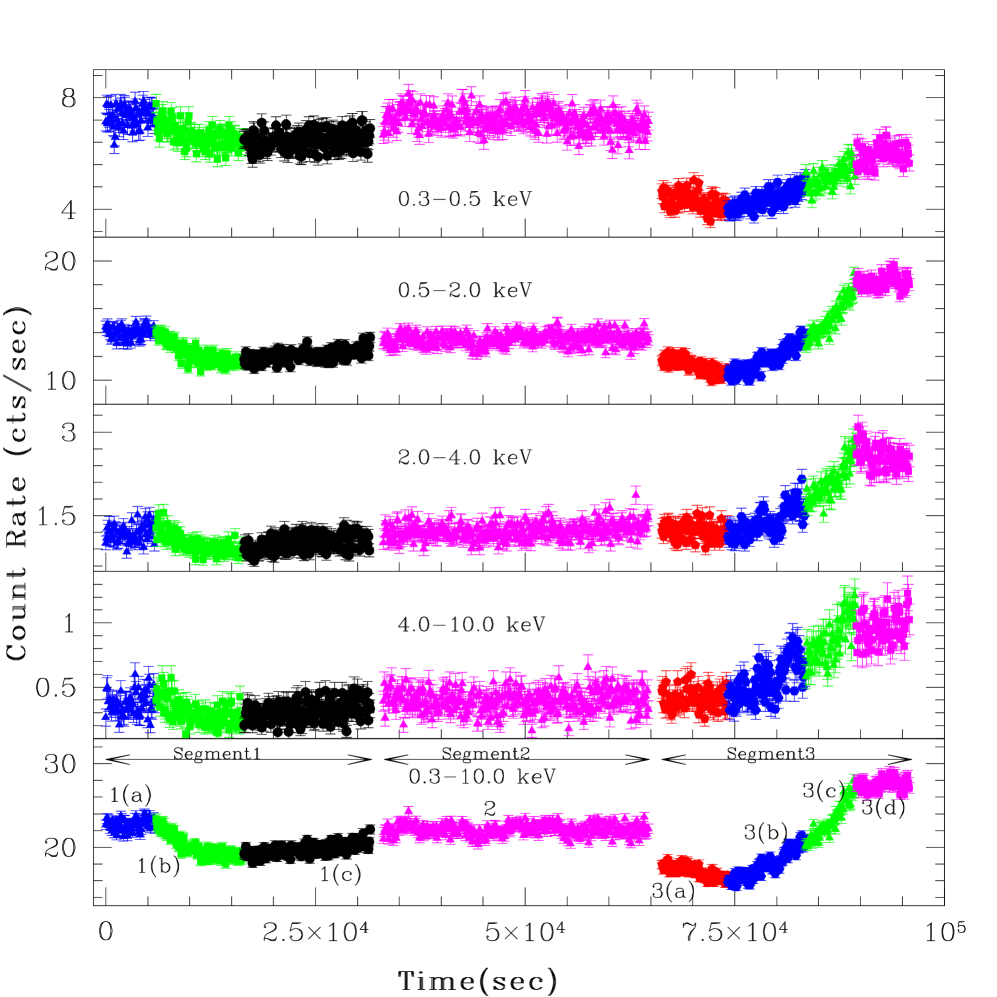
Figure 1: The background subtracted X-ray light curve of PKS 2155$-$304 in different energy bands.

We present the light curves extracted from entire observation of PKS 2155$-$304 in the five energy bands of 0.3 - 0.5 keV, 0.5 - 2.0 keV, 2.0 - 4.0 keV, 4.0 - 10.0 keV and 0.3 - 10.0 keV (with an 100 s binning) in Fig. 1. As mentioned above, this observation consists of three exposures with a duration 31.7, 31.6 and 29.7 ks, respectively. The gaps between the individual exposures are of the order of $\sim 1.5$ ks. The three sub-parts are easily spotted by the abrupt change in the source flux. For example, the flux drop at around $\sim 65$ ks since the start of the observation is not real, but is due to the change of the EPIC/pn filters, since the EPIC/pn thin filter is more transparent to the soft energy photons than the thick filter. A similar effect, but of a much smaller amplitude, is observed $\sim 30$ ks since the start of the observation, when the EPIC/pn filter was switched from medium to thin.

Despite the EPIC/pn filter changes, a visual inspection indicates significant and clearly defined flux variability in the light curve. In Fig. 1, the individual exposures are marked as segments 1, 2, and 3. We divided segment 1 into three sub-segments: 1(a) where the source flux is almost constant; 1(b) where the flux decreases; and 1(c) where the source flux rises. Segment 2 is relatively flat, but this is when the source has shown a hint of a QPO [14]. Segment 3 is divided into four sub-segments: 3(a), with decreasing flux, 3(d) corresponds to the $\sim$ constant flux level towards the end of the observation, while 3(b) and 3(c) are defined during the first and second part of the strong rising flux state in between. The percentage variability and signal to noise ratio (S/N) of segment 1, 2 and 3 in 0.3 – 10.0 keV band are 6.6$\pm$0.16, 1.5$\pm$0.22, 21$\pm$0.15 and 37.7, 39.3, 38.0, respectively.

3.2 Spectral Variability

To investigate if there are spectral variations associated with the well defined flux variations, we generated the spectra of the eight sub-segments we discussed above. We then fitted a simple power law (PL) model to the X-ray spectra using XSPEC (v. 12.8.0). The average value of Galactic neutral hydrogen absorption was found from the HEASARC N_H calculator to be $N_{H}=1.71\times 10^{20}$ cm^-2 [41]. We kept this value fixed in all spectral fits. The best model fit results (reduced $\chi^{2}$ values and model parameters with their corresponding 90% confidence intervals) are summarized in Table 1. In the last three columns of the same Table we list the best-fit flux estimates (together with their 90% confidence limits) in the 0.3-2, 2-10 and 0.3-10 keV bands. The best fit PL models, and ratios of data to model are plotted in Fig.  2 for all segments. Based on the null probability for the PL model fits (listed in the 7th column of the upper part of Table 1) the model provides statistically acceptable fits to the spectra of all segments. The exception are the spectral of segments 3(b) and 3(d), in particular, where the probability is low. The data-to-model ratios for segments 3(d)(bottom right panels in Fig. 2) show a convex shape above $\sim 2$ or $3$ keV. This shape is indicative of a more complex spectral shape.

For that reason, we also fitted the spectra with a broken power-law model (BKPL). The best BKPL model fit results are also listed in Table 1. The model resulted in entirely unconstrained break-energies, and almost identical $\Gamma_{1}$ and $\Gamma_{2}$ best fit values, in the case of segments 1(a), 1(b), 1(c). These results imply that a single PL model is adequate for the characterization of the energy spectra of these segments. For this reason, we do not list the BKPL best-fit results for these segments in Table 1. Contrary to this, the BKPL best-fit $\chi^{2}$ values are smaller than the respective PL best-fit values, for the remaining segments. The numbers in parenthesis in the 7th column of Table 1 indicate the probability of the $F-$statistic given the $\chi^{2}$ values of the PL and BKPL best-fits. Based on the $F-$ratio probabilities, the improvement in the fit when we consider the BKPL model is significant at more than the 99% level in the case of segment 2 and all sub-segments of the last part of the observation.

Our results indicate that during segments 2 and 3(a), when the flux remains rather constant, the spectra steepen above the break energy by an average $\Delta\Gamma=0.11\pm 0.08$. A stronger spectral steepening, by a factor of $\Delta\Gamma=0.55\pm 0.27$ is also observed during segment 3(d), when the flux remains again $\sim$ constant, albeit at a higher than previous level. In all these three cases, the break-energy is rather high, with an average value of $3.4\pm 0.7$ keV. On the contrary, the strong flux rise observed during segments 3b and 3c, is associated with a small, but significant, spectral hardening at high energies, of $\Delta\Gamma=-0.07\pm 0.02$, between the spectral slope below and above the break-energy. At the same time, the average break energy for these segments is $1.26\pm 0.32$, which is significantly smaller than the break-energy in the spectra of segment 3d.

“Log-parabolic” models have also been used to describe continuously downward-curving spectra of HSPs [42]. We fitted the spectra of all segments with such a model, but the quality of the fits is not significantly better than that of the PL fits. In fact, in some cases, the $\chi^{2}$ values are even larger than those from the PL fits (for a smaller number of dof). The best-fit curvature parameter turns out to be negative only for segments 1(b) and 1(c), but even in this case, the values are consistent with zero within the errors.

Using the PL best-fit results, we investigated whether the spectral variations are related with the flux variations of the source. Figure 3 shows a plot of the spectral PL indexas a function of the source 2–10 keV flux. In general, we find that the spectral slope is anti-correlated with flux; the spectra “harden” with increasing flux. Using the data plotted in Fig. 3, we find a correlation coefficient of $r=-0.95$, which is significant at better than the 99% confidence level ($P_{null}=3.0\times 10^{-4}$). Looking the data in more detail, the source flux and spectral index are similar for the first three segments (1a, 1b and 1c), while the spectral index flattens as the 2–10 keV flux increases during segments (2) and (3a). Taken as a whole, the spectral-flux evolution from (1a) to (3) may exhibit a “clockwise trajectory” in the “spectral slope – flux” plane, although the flux and spectral variations are not of very large amplitude. The spectrum shows a strong “hardening” during the strong flux rise towards the end of the observation.

3.3 Correlation Analysis

The spectral variations reported in the previous section suggest possible energy delays in the observed flux variations. In order to investigate further the spectral variability of the source, we estimated the Cross-Correlation Function (CCF) between light curves at different energy bands, using light curves with a 100 s bin size. We chose light curves in the energy bands 0.3–0.5, 0.5–2, 2–4 and 4–10 keV. We calculated the sample CCF as in Section 3 of [43], and we estimated the CCF between the 4–10, 2–4, and 0.5–2 keV band light curves versus the 0.3–0.5 keV band light curve. Significant correlation at positive lags means that soft (i.e. the 0.3–0.5 keV) band variations are leading the variations in the “harder” band.

We followed a similar, but simplified, version of the “sliding window ” technique of [43]. We calculated the CCFs for 10 ks intervals, which started at different times of the observed light curves. More specifically, we used 10 ks data streams which started at the points $t_{\rm start}=0,500,1000,\ldots$ s since the start of the observation. As a result, we computed the CCF for $\sim 170$ 10 ks long segments for the complete light curve. For each CCF, we identified the lag, $\tau_{\rm max}$, at which the CCF was maximum (i.e. CCF_max), and calculated the mean time lag, $\tau_{\rm mean}$, as the mean of the time lags of the points with CCF values larger or equal to 0.8$\times$CCF_max, in the case when: a) the CCF_max value was larger or equal to 0.8, and b) there were at least five points with a CCF value larger than 0.8 of CCF_max. In other words, we have only considered CCF peaks which are strong, broad and well defined, as opposed to random, narrow peaks in the CCF. Finally, we did not consider light curve segments in the time intervals between 21.7-43 ks and 54.6-76 ks after the start of the observation, as in this case, the light curves would include data during the EPIC/pn filter switches (which affect in a different way the observed count rate in the soft and harder energy bands).

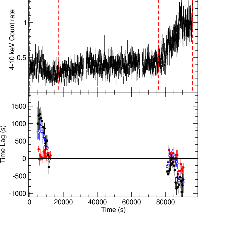
Figure 4: The 4–10 keV band light curve (top panel) together with the temporal variation of the delays between the 0.3–0.5 keV band light curve and the 0.5–2, 2–4 and 4-10 keV band light curves, in the bottom panel (red filled circles, blue open circles and black field circles, respectively).

The above procedure allows us to monitor the temporal variation of the time lag between various bands. Our results are plotted in Fig.  4. The top panel in this figure shows the 4–10 keV band light curve (which is the most representative of the intrinsic source variations, as this band is less affected by the filter changes). The bottom panel shows the average time lag between the 0.5–2, 2–4 and 4–10 keV band light curves and the 0.3–0.5 keV band light curve (red filled circles, blue open circles, and black filled circles, respectively). The vertical dashed lines in the top panel indicate the light curve segments that were used to estimate the mean time lags plotted in the bottom panel. In addition to the intervals that we excluded for the estimation of the CCF, the resulting CCF for the intervals $\sim 17-22$ ks and $43-55$ ks did not show any significant peaks in them. This is most probably due to the fact that all light curves were relative flat during these periods, with very low amplitude variations, roughly similar to the Poisson noise variations (specially in the high energy bands). Consequently, the sample CCFs are not capable to detect any intrinsic delays in these periods.

Our results indicate that the correlation between the “soft” and “hard” bands is rather complex. In the first part of the observation (the part which corresponds to segments (1a), (1b) and the first part of segment (1c) the lags are positive, i.e. the variations in the 0.3–0.5 keV band are leading those in the harder bands (i.e. we observe a hard lag). In this case, whatever the characteristic time scales which dominate the observed variations, they must be faster at low energies. Furthermore, the time lags between the highest energy bands (4–10 and 2–10 keV) and 0.3–0.5 keV appear to decrease with time, from $\sim 1.5$ to $\sim 0$ ks. At the same time, the 0.5–2 vs 0.3–0.5 keV lags appear to be constant at $\sim 100$ s.

The reverse situation is observed in the last part of the observation, $\sim 80$ ks after the start of the observation, during the continuous, large amplitude flux rise. During the flux rise, the time delays between 0.5–2 and 0.3–0.5 keV, as well as between the 2–4 and 0.3–0.5 keV bands are consistent with zero, while the 4–10 keV band variations may be leading the soft band variations. When the source flux flattens after $\sim 85$ ks, the harder band variations are clearly leading the soft band variations (i.e. we observe a soft lag). The delay is energy dependent: the 0.3–0.5 keV band variations are delayed with respect to the 4–10 and 2–4 keV band variations by $\sim 700$ s, while the time lag between the 0.5–2 and the 0.3–0.5 keV bands is $\sim 300$ s .

curve and the 0.5–2, 2–4 and 4-10 keV band light curves, in the bottom panel (red filled circles, blue open circles and black field circles, respectively).

curve respectively).

4 Discussion and Conclusions

We have studied the flux and spectral variability of PKS 2155–304 using a $\sim 100$ ks XMM/Newton observation. The flux variability detected in this observation is rather typical of this source; we observe a short flare, decaying and stable flux states, as well as a rapid, large amplitude flux increase towards the end of the observation. We performed a time-resolved spectroscopic analysis, by dividing the data in various segments with different mean flux, and we fitted a simple power-law model to them.

4.1 The spectral variability results

In general, X-ray spectra of HSPs are rather steep $(\Gamma~{}\textgreater~{}2)$ and continuously steepen with increasing energies [44,45]). As a result, X-ray spectra of HSPs follow a convex, or continuously downward-curved, shape. This is a signature of the high energy tail of synchrotron emission that is the outcome of energy dependent particle acceleration and cooling [42]. In the last decade, X-ray observations of PKS 2155–304 by various X-ray telescopes have shown that its spectra normally has a convex shape below 10 keV [39,46-49]. However, two observations by XMM-Newton of this blazar in 2006 were analyzed by [38] and he reported that the shape of those X-ray spectra were concave.

Our observations indicate that a simple power-law model can describe adequately the source’s spectra during the first part of the observation, when we observe a mini-flare. In the rest of the observation, our analysis indicate that the energy spectra are more complex. We observe a spectral steepening above $\sim 3.4$ keV, by a factor of $\Delta\Gamma\sim 0.1-0.5$ during segments 2, 3(a) and 3(d), when the flux remains rather constant.

In addition, during the flux rise detected towards the end of the observation (segments 3b and 3c) the X-ray spectra show the opposite behavior; we observe a spectral hardening, of low amplitude ($\Delta\Gamma\sim 0.1$, above $\sim 1-1.5$ keV. This could be an indication of the low-energy side of the Inverse Compton emission contributing to energies even below 10 keV. A detailed, similar analysis of all the available XMM-Newton observations of the source, could provide useful information regarding the spectral hardening/softening (amplitude of $\Delta\Gamma$ and location of $E_{\rm break}$) and its relation to the flux variations of the source.

When we plotted the spectral index as a function of flux, we found the typical “flatter when brighter” spectral variability behavior, in agreement with previous studies [28,32,48]. This anti-correlation between spectral slope and source flux is a signature of spectral flattening with increasing flux, and indicates that the hard X-ray band flux increases more than the soft X-ray band flux as the flux increases. There is an indication of spectral variations along a “clockwise” trajectory on the spectral slope – flux plane, but the evidence is not very strong.

4.2 The cross-correlation results

We also performed a detailed cross-correlation analysis of the variations detected, by dividing the light curve into 4 energy bands. We detected both hard lags, as well as soft lags, in the first and last part of the observation, respectively. To the best of our knowledge, this is the first time that both hard and soft lags are detected in a light curve of this source.

In the simplest case scenario, the X-ray emission variation of HSPs is controlled by the energy dependent particle acceleration and cooling mechanisms. The cooling process is well understood but particle acceleration is not well understood yet and could operate in different ways [50,51]. Following [51], the acceleration timescale, $t_{\rm acc}$, of the relativistic electrons, and their cooling time scale, $t_{\rm cool}$, in the observed frame, can be expressed as a function of the observed photon energy E (in keV) as follows:

$$t_{\rm acc}(E)=9.65\times 10^{-2}(1+z)^{3/2}\xi B^{-3/2}\delta^{-3/2}E^{1/2}{\rm s},$$ (1)

and,

$$t_{\rm cool}(E)=3.04\times 10^{3}(1+z)^{1/2}B^{-3/2}\delta^{-1/2}E^{-1/2}{\rm s},$$ (2)

where $z$ is the source red shift, $B$ is the magnetic field (in Gauss), $\delta$ is the Doppler factor of the emitting region, and $\xi$ is a parameter describing how fast the electron can be accelerated.

Equations (1) and (2) show that both $t_{\rm cool}$ and $t_{\rm acc}$ depend on the observed photon energy but do so in an inverse fashion. The lower energy electrons are radiating low energy photons which cool slower but are accelerated faster than the high energy electrons that are radiating the high energy photons. The relationship between $t_{\rm cool}$ and $t_{\rm acc}$ can in principle give an important clue about the process that dominates the X-ray emission.

If $t_{\rm cool}$ is significantly larger than $t_{\rm acc}$, the cooling process dominates [52]. In this case, any change in emission will propagate from higher to lower energies so that higher energy photons will lead lower energy photons (soft lag) and a clockwise loop of spectral index against the flux will be observed. The expected soft lag should be approximately equal to

$$\tau_{\rm soft}=t_{\rm cool}(E_{\rm l})-t_{\rm cool}(E_{\rm h}),$$ (3)

where $\tau_{\rm soft}$ is the observed soft lag, and the values of $E_{\rm l}$ and $E_{\rm h}$ are the energy of the lower and higher energy bands in units of keV, respectively.

In contrast, if $t_{\rm acc}$ is comparable to the $t_{\rm cool}$ in the observed energy range, the system is dominated by acceleration processes and any variation in emission propagates from lower to higher energies because it takes a longer time to accelerate a particle to higher energies. In this case there would be a hard lag and an anti-clockwise loop would be observed in spectral index versus flux plot. The time lag in an acceleration dominated system is expressed as,

$$\tau_{\rm hard}=t_{\rm acc}(E_{\rm h})-t_{\rm acc}(E_{\rm l}),$$ (4)

where $\tau_{\rm hard}$ is the observed hard lag between the low and high energy bands, respectively.

4.3 Implications of the hard lags

Based on this scenario, the hard lag we observe in the first part of the observation may indicate that the system is dominated by acceleration processes. We observe that $\tau_{hard}(4-10{\rm vs}0.3-0.5)>\tau_{hard}(2-4{\rm vs}0.3-0.5)>\tau_{hard}(0.5-2{\rm vs}0.3--0.5)$, which is easy to understand since the energy separation of these bands increases accordingly. Using equations (1) and (4), we can show that, in this case, we should expect that

$$B\delta\xi^{-2/3}=0.21(1+z)E_{h}^{1/3}\left[\frac{1-(E_{l}/E_{h})^{1/2}}{\tau_{\rm hard}}\right]^{2/3}.$$ (5)

We found that $\tau_{hard}(4-10{\rm vs}0.3-0.5)$ and $\tau_{hard}(2-4{\rm vs}0.3-0.5)$ do not remain constant, but rather decrease with time. According to eq. (5), this would imply that either $B$ and/or $\delta$ increase with time, or that the parameter $\xi$ decreases with time. We also observed that $\tau_{hard}(0.5-2{\rm vs}0.3-0.5)$ to remain constant in the same period. This result indicates that neither $B$ nor $\delta$ should control the variations with time of the $\tau_{hard}$ in the higher energy bands, as in this case we would expect these lags to decrease with time.

One possibility is that the acceleration process dominates the variations above 2 keV, but at lower energies a different variability process dominates the observed variations. This is though highly unlikely, given the very good correlation between the variations below and above 2 keV. Perhaps then,the variability in the first part of the observation is dominated by acceleration process, and that the rate of acceleration, $\xi$, does not remain constant, but rather decreases with time. In addition, if a variable $\xi$ determines the variability evolution of the system then, apart from being time dependent, it may also by energy dependent, in which case the constant low-energy time lags could also be explained.

The probability of the system to be “acceleration dominated” contradicts the spectral slope - flux evolution in the first part of the observation. Our spectral analysis suggests a clockwise trajectory in the spectral index versus flux plot during the first part of the observation. Arguably the amplitude of this “trajectory” is not very strong, but it is fair to notice that we find no evidence of an “anti-clockwise” evolution, which is what we would expect if the acceleration process dominates the variability evolution of the source. We cannot offer an interpretation at the moment, as to why could be the reason for these seemingly contradictory results.

4.4 Implications of the soft lags

On the other hand, the soft lags we observe in the last part of the observation suggest that the system is dominated by cooling processes. We observe again that $\tau_{hard}(4-10{\rm vs}0.3-0.5)>\tau_{hard}(2-4{\rm vs}0.3-0.5)>\tau_{hard}(0.5-2{\rm vs}0.3-0.5)$ (in absolute value), which can be again understood due to the accordingly increasing energy separation of these bands. Using equations (2) and (3), we expect that, in this case,

$$B\delta^{1/3}=209.91\left(\frac{1+z}{E_{l}}\right)^{1/3}\left[\frac{1-(E_{l}/E_{h})^{1/2}}{\tau_{soft}}\right]^{2/3}.$$ (6)

The above equation indicates that the observed time lags should be inversely proportional either to the magnetic field $B$ of the emitting blob ($B\propto\tau^{-2/3}$) and/or to $\delta$ ($\delta\propto\tau^{-2/3}$). In the last part of the observation, we observe that all soft lags remain roughly constant. Their (absolute) mean values at times longer than 85 ks (since the start of the observation) are: $<\tau_{soft}(4-10{\rm vs}0.3-0.5)>=726\pm 54$ s, $<\tau_{soft}(2-4{\rm vs}0.3-0.5)>=625\pm 25$ s, and $<\tau_{soft}(0.5-2{\rm vs}0.3-0.5)>=317\pm 36$ s. Assuming that $\delta t=10$ and that it remains constant during the observation, then the above values together with eq. (6), result in the following estimates for the magnetic field strength: $1.8\pm 0.2$ G, $1.5\pm 0.05$ G, and $1.5\pm 0.1$ G. The weighted mean value is $1.5\pm 0.05$ G, which is similar to the magnetic field values that result from the broad band SED fitting of blazars [53]. We note that, according to our results, $\tau_{soft}$ is much smaller by a factor of $\sim 5-6$ (for all energy bands) during the flux rise (at times $\sim 75-85$ ks). This would imply an increased magnetic field value, by a factor of $\sim 3$ during the flux rise phase.
(28) have analyzed the same observations and done cross correlation analysis in which they divided the each exposure light curve in three energy (e.g., 0.2-0.8 keV (soft), 0.8.2.4 keV (medium) and 2.4-10.0 keV (hard)) bands. In their analysis they have calculated the time lags between soft/medium and soft/hard energy bands. They have found the soft band variations lag behind the medium and hard band by $\sim 450\pm 300$, $\sim 870\pm 540$ and $\sim 420\pm 180$, $\sim 1280\pm 240$ seconds, respectively in segment 1 and 3 of the light curves. Our results are comparable to these results in segment 3 and opposite in segment 1.

4.5 Summary

Our analysis suggest the presence of soft lags in some epochs and hard lags in other epochs, during the May 2002 XMM-Newton observation of PKS 2155-304. This result implies that the difference between $t_{\rm acc}$ and $t_{\rm cool}$ of the emitting electrons is changing from epoch to epoch, in agreement with past studies [28,48,49].

Hard time lags are detected during the first part of the observation. These lags suggest that the flux evolution during this part of the observation is dominated by the acceleration process. These delays may be modulated by variations of the acceleration parameter $\xi$ in time, and perhaps in energy as well). The shock formation process due to collision is the most acceptable reason for particle acceleration [54,55]. If real, the variation in the value of $\xi$ indicates that the particle acceleration mechanisms may be time variable. Using the soft time lags observed in the last part of the observation we have estimated the value of the magnetic field, which turns out to be similar to the values that have been reported in the literature, based on the modeling of the full band SEDs of blazars. We also found evidence for the magnetic field variations, during the flux rise phases in the light curve.

The X-ray observations are the most powerful diagnostic tool for blazars which have an ability to provide information about the physical processes taking place in the vicinity of the central engines of these sources. We believe that our results demonstrate that, in order understand the relationship between particle acceleration and cooling, combined spectral and timing studies within the X–ray band can be useful. Future, similar studies of the archival XMM/Newton observations of this source may allow us to understand better the physical processes that control the flux and spectral variations in this source.

Table 1. Results of X-ray spectral fits to PKS 2155$-$304

Segment $\Gamma_{1}$ N^a E_break $\Gamma_{2}$ ${\chi^{2}}$/dof Prob. Flux^b Flux^c Flux^d Power-Law (PL) Model 1(a) 2.66${}_{-0.01}^{+0.01}$ 3.04${}_{-0.02}^{+0.02}$ … … 151.8/142 0.27 1.010${}_{-0.004}^{+0.003}$ 0.305${}_{-0.003}^{+0.003}$ 1.315${}_{-0.005}^{+0.004}$ 1(b) 2.70${}_{-0.01}^{+0.01}$ 2.65${}_{-0.01}^{+0.01}$ … … 157.1/157 0.48 0.898${}_{-0.002}^{+0.002}$ 0.250${}_{-0.002}^{+0.002}$ 1.148${}_{-0.003}^{+0.003}$ 1(c) 2.68${}_{-0.01}^{+0.01}$ 2.63${}_{-0.01}^{+0.02}$ … … 185.0/177 0.34 0.882${}_{-0.002}^{+0.002}$ 0.255${}_{-0.002}^{+0.002}$ 1.137${}_{-0.003}^{+0.003}$ 2 2.58${}_{-0.01}^{+0.01}$ 2.86${}_{-0.01}^{+0.01}$ … … 222.5/207 0.22 0.921${}_{-0.001}^{+0.001}$ 0.320${}_{-0.001}^{+0.001}$ 1.241${}_{-0.002}^{+0.002}$ 3(a) 2.56${}_{-0.01}^{+0.01}$ 3.04${}_{-0.02}^{+0.02}$ … … 172.4/156 0.17 0.973${}_{-0.003}^{+0.004}$ 0.347${}_{-0.003}^{+0.003}$ 1.321${}_{-0.005}^{+0.004}$ 3(b) 2.46${}_{-0.01}^{+0.01}$ 3.16${}_{-0.02}^{+0.02}$ … … 205.8/174 0.05 0.976${}_{-0.004}^{+0.004}$ 0.420${}_{-0.003}^{+0.003}$ 1.395${}_{-0.004}^{+0.005}$ 3(c) 2.32${}_{-0.01}^{+0.01}$ 4.12${}_{-0.02}^{+0.02}$ … … 182.9/178 0.38 1.217${}_{-0.004}^{+0.004}$ 0.676${}_{-0.005}^{+0.006}$ 1.885${}_{-0.007}^{+0.007}$ 3(d) 2.32${}_{-0.01}^{+0.01}$ 4.89${}_{-0.02}^{+0.02}$ … … 247.3/179 5.5e-4 1.444${}_{-0.005}^{+0.004}$ 0.793${}_{-0.006}^{+0.006}$ 2.236${}_{-0.005}^{+0.007}$ Broken-Power-Law (BKPL) Model 2 2.58${}_{-0.01}^{+0.01}$ 2.86${}_{-0.01}^{+0.01}$ 3.27${}_{-0.78}^{+2.16}$ 2.65${}_{-0.04}^{+0.17}$ 210.7/205 0.38 0.921${}_{-0.001}^{+0.002}$ 0.315${}_{-0.002}^{+0.002}$ 1.236${}_{-0.002}^{+0.003}$ (4.0e-3) 3(a) 2.55${}_{-0.02}^{+0.01}$ 3.05${}_{-0.02}^{+0.02}$ 2.95${}_{-1.50}^{+0.83}$ 2.69${}_{-0.09}^{+0.10}$ 160.3/154 0.35 0.972${}_{-0.003}^{+0.003}$ 0.338${}_{-0.004}^{+0.005}$ 1.310${}_{-0.004}^{+0.007}$ 4.0e-3 3(b) 2.49${}_{-0.02}^{+0.02}$ 3.13${}_{-0.03}^{+0.02}$ 1.26${}_{-0.25}^{+0.60}$ 2.42${}_{-0.03}^{+0.02}$ 190.4/172 0.16 0.977${}_{-0.003}^{+0.004}$ 0.431${}_{-0.004}^{+0.003}$ 1.408${}_{-0.005}^{+0.007}$ (1.2e-3) 3(c) 2.35${}_{-0.02}^{+0.03}$ 4.08${}_{-0.07}^{+0.03}$ 1.26${}_{-0.44}^{+0.50}$ 2.28${}_{-0.02}^{+0.02}$ 170.2/176 0.61 1.220${}_{-0.005}^{+0.005}$ 0.683${}_{-0.006}^{+0.009}$ 1.902${}_{-0.007}^{+0.011}$ (1.8e-3) 3(d) 2.30${}_{-0.01}^{+0.01}$ 4.90${}_{-0.02}^{+0.02}$ 4.93${}_{-1.15}^{+0.47}$ 2.85${}_{-0.31}^{+0.22}$ 196.3/177 0.15 1.442${}_{-0.004}^{+0.005}$ 0.761${}_{-0.007}^{+0.008}$ 2.203${}_{-0.008}^{+0.010}$ (1.3e-9)
^a Normalization constant in units of 10^-2 photon cm^-2s^-1keV^-1
b Unabsorbed 0.3–2.0 keV model flux in units of 10^-10 erg cm^-2 s^-1
c Unabsorbed 2.0–10.0 keV model flux in units of 10^-10 erg cm^-2 s^-1
d Unabsorbed 0.3–10.0 keV model flux in units of 10^-10 erg cm^-2 s^-1

Figure 2: The pn count rate spectra corresponding to the various segments of observation ID 0124930501 with best fitting simple power-law models and data-to-model ratios. Top row (left to right) have sub-segment 1(a) & 1(b); second row have 1(c) & 2; third row 3(a)& 3(b) and the last row 3(c)& 3(d).

Figure 3: Photon-index versus the 2.0-10.0 keV flux

References

- [1] Ulrich, Maraschi, & Urry, 1997 ARA&A 35, 445.
- [2] Urry, C. M., Padovani, P., 1995. PASP 107, 803.
- [3] Ghisellini, G. et al., 1997. A&A 327, 61.
- [4] Abdo, A. A. et al., 2010. ApJ 716, 30.
- [5] Maraschi, L., Ghisellini, G., Celotti, A., 1992. ApJ 397, L5.
- [6] Ghisellini, G. et al., 1993. ApJ 407, 65.
- [7] Hovatta, T. et al., 2009. A&A 494, 527.
- [8] Wagner, S. J., Witzel, A., 1995. ARA&A 33, 163.
- [9] Gupta, A. C. et al., 2004. A&A 422, 505.
- [10] George, I. M., Warwick, R. S., Bromage, G. E., 1988. MNRAS 232, 793.
- [11] Giommi et al., 1990 ApJ, 356, 432.
- [12] Sambruna, R. M. et al., 1994. ApJ 434, 468.
- [13] Kohmura, Y. et al., 1994. PASJ 46, 131.
- [14] Gaur, H. et al., 2010. ApJ 718, 279.
- [15] Carini, M. T., Miller, H. R., 1992. ApJ 385, 146.
- [16] Urry, C. M. et al., 1993. ApJ 411, 614.
- [17] Urry, C. M. et al., 1997. ApJ 486, 799.
- [18] Brinkmann, W. et al., 1994. A&A 288, 433.
- [19] Courvoisier, T. J.-L. et al., 1995. ApJ 438, 108.
- [20] Edelson, R. A. et al., 1995. ApJ 438, 120
- [21] Pesce, J. E. et al., 1997. ApJ 486, 770.
- [22] Pian, E. et al., 1997. ApJ 486, 784.
- [23] Marshall, H. L. et al., 2001. ApJ 549, 938.
- [24] Aharonian, F. et al., 2005. A&A 442, 895.
- [25] Aharonian, F. et al., 2009. ApJ 696, L150.
- [26] Dominici, T. P., Abraham, Z., Galo, A. L., 2006. A&A 460, 665.
- [27] Zhang et al., 2005 ApJ 629, 686.
- [28] Zhang, Y.-H. et al., 2006. ApJ 637, 699.
- [29] Dolcini, A. et al., 2007. A&A 469, 503.
- [30] Piner, B. G., Pant, N., Edwards, P. G., 2008. ApJ 678, 64.
- [31] Sakamoto, Y. et al., 2008. ApJ 676, 113.
- [32] Kapanadze et al., 2014. MNRAS 444, 1077
- [33] H.E.S.S. Collaboration et al., 2012. A&A 539, 149.
- [34] Kastendieck, M. A., Ashley, M. C. B., Horns, D., 2011. A&A 531, A123.
- [35] Lachowicz, P. et al., 2009. A&A 506, L17.
- [36] Morini, M. et al., 1986. ApJ 306, L71.
- [37] Sembay, S. et al., 1993. ApJ 404, 112.
- [38] Zhang, Y. H., 2008. ApJ 682, 789.
- [39] Massaro, E. et al., 2008. A&A 478, 395
- [40] Bhagwan et al., 2014. MNRAS 444, 3647.
- [41] Dickey, J. M., Lockman, F. J., 1990. ARA&A 28, 215.
- [42] Massaro, E. et al., 2004. A&A 413, 489.
- [43] Brinkmann W. et al., 2005. A&A 443, 397
- [44] Perlman, E. S. et al., 2005. ApJ 625, 727.
- [45] Tramacere, A. et al., 2007. A&A 467, 501.
- [46] Foschini, L. et al., 2006. A&A 453, 829.
- [47] Kataoka, J. et al., 2000. ApJ 528, 243.
- [48] Zhang, Y. H., 2002. APJ 572, 762
- [49] Aharonian F. et al., 2009. A&A 502, 749
- [50] Katarzyński, K. et al., 2005. A&A 433, 479.
- [51] Zhang, Y. H., 2002. MNRAS 337, 609
- [52] Kirk, J. G., Rieger, F. M., Mastichiadis, A., 1998. A&A 333, 452.
- [53] Ghisellini G. et al., 2010. MNRAS 402, 497
- [54] Spada M. et al., 2001. MNRAS 325, 1559
- [55] Mimica P. et al., 2005. A&A 441, 103