An $R$-matrix package for coupled-channel problems in nuclear physics

Abstract

We present an $R$-matrix Fortran package to solve coupled-channel problems in nuclear physics. The basis functions are chosen as Lagrange functions, which permits simple calculations of the matrix elements. The main input are the coupling potentials at some nucleus-nucleus distances, specified by the program. The program provides the collision matrix and, optionally, the associated wave function. The present method deals with open and closed channels simultaneously, without numerical instability associated with closed channels. It can also solve coupled-channel problems for non-local potentials. Long-range potentials can be treated with propagation techniques, which significantly speed up the calculations. We first present an overview of the $R$-matrix theory, and of the Lagrange-mesh method. A description of the package and its installation on a UNIX machine is then provided. Finally, five typical examples are discussed.

PROGRAM SUMMARY

Manuscript Title: An $R$-matrix package for coupled-channel problems in nuclear physics
Author: P. Descouvemont
Program Title: rmatrix
Journal Reference:
Catalogue identifier:
Licensing provisions: none
Programming language: Fortran 90
RAM: memory usage strongly depends on the nature of the problem (number of channels, size of the basis).
Keywords: scattering theory, $R$-matrix method, Lagrange meshes, coupled-channel problems.
Classification: 17.8 Nuclear Reaction - General
External routines/libraries: if available, the LAPACK library can be used for matrix inversion (faster than the subroutine included in the package).
Nature of problem: solving coupled-channel problems for positive energies; the package provides the collision matrix and the associated wave function for given energy, spin and parity.

Solution method: the coupled-channel system is solved with the $R$-matrix method, and Lagrange functions are adopted. Propagation of the $R$-matrix can be performed.
Restrictions: for non-local potentials, the propagation technique cannot be used.
Running time: strongly depends on the nature of the problem. For single-channel calculations, the running type is typically less than 1 s. For large scale calculations (typically more than 100 channels), the running time may increase up to several minutes on a multi-CPU Linux machine.

1 Introduction

Many problems in quantum physics require the solution of a second-order differential system. Nuclear [1, 2, 3] and atomic [4, 5, 6] collisions are obvious examples (see also Ref. [7]). Solving a coupled-channel system is also necessary in other applications, such as the description of three-body systems [8, 9]. The Resonating Group Method (RGM, see Ref. [10]) is used in nuclear physics to describe nucleus-nucleus collisions from $A$-body wave functions, and takes antisymmetrization exactly into account. It provides a system involving non-local potentials [10, 11, 12].

Solving a coupled-channel system for bound states, i. e. for energies below all threshold energies, is relatively simple, and can be addressed by different methods (see, for example, Ref. [13]). In particular, variational methods using large bases [14, 15, 16] provide accurate solutions for bound-state problems. Various improvements, such as a random selection of the basis functions [17], have been proposed to optimize the choice of basis states. The main difficulty in bound-state calculations is to deal with the diagonalization of extremely large bases.

Scattering states, however, are more complicated owing to the long range behavior of the wave functions. Finite-difference methods, based on the Numerov algorithm [18, 19, 20], can be used to integrate the system until large distances, where the wave function reaches its asymptotic behaviour. The matching to Coulomb functions then provides the collision matrix, which is subsequently used to compute various cross sections. In contrast, the $R$-matrix method is a well-established tool to complement variational calculations, frequently used to define bound states, to scattering states. However, as variational calculations involve square integrable functions, any finite combination tends to zero at large distances.

The original idea of the $R$-matrix method is due to Wigner [21] with the aim of describing resonances. The $R$-matrix theory describes scattering states between interacting particles, which can be nuclei, atoms, molecules. It is based on the division of the configuration space in two regions. In the internal region, both particles interact through some potential, which depends on the model. In the external region, possible antisymmetrization effects and non-monopole Coulomb terms are neglected. The border is called the channel radius and must be chosen large enough to comply with these requirements. Extensions to the scattering of three particles have been developed [22, 23], but will not be presented here. Three-body continuum wave functions are required, for example, in breakup calculations [24].

The $R$-matrix method has been presented in many reviews or books. It has been developed both in atomic [6] and nuclear [25, 26] physics. As basis functions, we use here Lagrange functions [27] which permit fast calculations of the matrix elements [28, 26]. Another important advantage is that non-local potentials are easily implemented [29]. In addition, closed channels are treated in a straightforward way, in contrast with finite-difference methods, where the exponentially growing component raises strong numerical problems. Our main goal here is to provide the user with an efficient routine, which can be easily implemented in any code, as soon as the coupling potentials are known. Previous codes are essentially focused on atomic physics or only consider propagation of the $R$-matrix across several intervals [30, 31, 4].

Notice that the $R$-matrix theory can be used in another variant, known as the phenomenological $R$-matrix [25, 32, 26]. Although the origins of both variants are common, the goal of the phenomenological approach is to fit the $R$-matrix parameters to experimental data, such as elastic-scattering or radiative-capture cross sections. This variant is essentially used to determine resonance parameters at low energies and, in nuclear astrophysics, to extrapolate cross sections down to stellar energies, where, in general, no data exist.

We present first a brief overview of the $R$-matrix theory in Section 2. Sections 3 and 4 provide a description of the package. We give typical examples in Section 5, with the outputs presented in Appendices. Concluding remarks are presented in Section 7.

2 Brief overview of the $R$-matrix method

2.1 The collision matrix

We present here a short description of the theory, and we refer the reader to Refs. [6, 26] for more detail. Let us consider a coupled-channel system for two particles

$$\sum_{j=1}^{N_{c}}\bigl{(}T_{i}\delta_{ij}+V_{ij}(r)\bigr{)}u_{j}(r)=(E-E_{i})u_{i}(r),$$ (1)

where $r$ is the relative coordinate, $N_{c}$ is the number of channels, $E$ is the scattering energy, and $E_{i}$ is the threshold energy of channel $i$. Notice that we define a “channel” as characterized by a threshold energy $E_{i}$ and by an orbital angular momentum $L_{i}$. This definition is well adapted to numerical aspects. However, it should not be confused with “physical channels”, characterized by the quantum numbers (energy, spin and parity) of the colliding nuclei. We assume that all energies $(E,E_{i})$ are given with respect to $E_{\omega}$, the energy of the entrance channel $\omega$.

In (1), $V_{ij}(r)$ are the coupling potentials (symmetric), which may be real or complex. The kinetic-energy operator reads

$$T_{i}=-\frac{\hbar^{2}}{2\mu}\biggl{(}\frac{d^{2}}{dr^{2}}-\frac{L_{i}(L_{i}+1)}{r^{2}}\biggr{)},$$ (2)

where $\mu$ is the reduced mass (we assume that it does not depend on the channel), and $L_{i}$ the orbital momentum in channel $i$. For the sake of clarity we consider now local potentials only, but a generalization to non-local potentials is possible, and will be presenter later.

As mentioned in the introduction, the coupling potentials may originate from various models. However, the $R$-matrix method is a tool to solve (1) for the continuum, and does not depend on the physics of the problem. The main requirement is that, at large distances, the potentials tend to

$$V_{ij}(r)\rightarrow\frac{Z_{1}Z_{2}e^{2}}{r}\delta_{ij},$$ (3)

where $Z_{1}e$ and $Z_{2}e$ are the charges of the colliding nuclei. This assumption implicitly defines the lower limit for the choice of the channel radius.

For a bound state, all channels are closed $(E<E_{i})$, and long-range contributions to the wave function are, in general, neglected. A scattering state (including resonances) is characterized by at least one open channel. At large distances, i. e. when Eq. (3) is valid, the solutions of the coupled-channel system (1) are given by

$$u_{i,\rm ext}^{\omega}(r)=\left\{\begin{array}[]{ll}v_{i}^{-1/2}\Bigl{(}I_{L_{i}}(k_{i}r)\delta_{i\omega}-O_{L_{i}}(k_{i}r)U_{i\omega}\Bigr{)}&{\rm\ for\ }E>E_{i},\\ A_{i}^{\omega}W_{-\eta_{i},L_{i}+1/2}(2k_{i}r)&{\rm\ for\ }E<E_{i}.\end{array}\right.$$ (6)

In these definitions, $v_{i}$ and $k_{i}$ are the velocity and wave number in channel $i$ $(k_{i}^{2}=2\mu|E-E_{i}|/\hbar^{2})$, and $\omega$ is the entrance channel. Functions $I_{L_{i}}(x)$ and $O_{L_{i}}(x)$ are the incoming and outgoing Coulomb functions [33], and $W_{a,b}(x)$ is the Whittaker function [34]. Equations (6) define the collision matrix $\boldsymbol{U}$, which is used to compute cross sections [3, 7]. The collision matrix is symmetric, and unitary for real potentials. The other output from the calculations are the amplitudes of closed channels $A_{i}^{\omega}$. Although some solutions have been proposed in the literature (see e.g. Ref. [19]), including closed channels in finite-difference methods raises numerical problems, due to the exponential behaviour of the associated wave-function components. At energies close to breakup channels, however, closed channels may be expected to play a significant role. In the $R$-matrix theory, open and closed channels are treated on an equal footing.

Notice that, in the literature, matrix $\boldsymbol{U}$ is also called the scattering matrix. We follow here the naming used by Lane and Thomas [25]. Another important comment deals with the normalization (6). This choice ensures that the collision matrix is symmetric. An alternative is to define the asymptotic part of open-channel components as

$$u_{i,\rm ext}^{\omega}(r)=v_{\omega}^{-1/2}\biggl{(}I_{L_{i}}(k_{i}r)\delta_{i\omega}-O_{L_{i}}(k_{i}r)\tilde{U}_{i\omega}\biggr{)},$$ (7)

with

$$\tilde{U}_{ij}=\biggl{(}\frac{k_{j}}{k_{i}}\biggr{)}^{1/2}U_{ij}.$$ (8)

This choice is adopted, for example, in Ref. [3]. In that case, matrix $\tilde{\boldsymbol{U}}$ is not symmetric.

The basic idea of the $R$-matrix method is to solve system (3) on a limited interval, defined by the channel radius $a$. In the internal region $(r\leq a)$, the wave functions are expanded over $N$ basis states $\varphi_{n}(r)$ as

$$u_{i,\rm int}^{\omega}(r)=\sum_{n=1}^{N}f^{\omega}_{in}\,\varphi_{n}(r).$$ (9)

These basis functions can be orthogonal or not. The unknown quantities of a scattering problem are therefore the coefficients $f^{\omega}_{in}$, the collision matrix $U_{ij}$, and the closed-channel amplitudes $A_{i}^{\omega}$. These quantities are obtained from the $R$-matrix theory as described below.

The kinetic-energy operator is not hermitian over a finite range $[0,a]$. This issue is solved by introducing the Bloch operator [35]

$${\cal L}(B_{i})=\frac{\hbar^{2}}{2\mu}\delta(r-a)\biggl{(}\frac{d}{dr}-\frac{B_{i}}{r}\biggr{)},$$ (10)

which is also called surface operator since it acts at $r=a$ only. Constants $B_{i}$ are boundary-condition parameters, and may depend on the channel. For real $B_{i}$ values, the operator $T_{i}+{\cal L}(B_{i})$ is hermitian over the interval $[0,a]$. These parameters are chosen here as

$$B_{i}=\left\{\begin{array}[]{ll}0&{\rm\ for\ open\ channels},\\ 2k_{i}a\frac{W^{\prime}(2k_{i}a)}{W(2k_{i}a)}&{\rm\ for\ closed\ channels},\end{array}\right.$$ (13)

where the prime denotes the derivative with respect to the argument $2k_{i}a$.

In the $R$-matrix approach, system (1) is therefore replaced by the Bloch-Schrödinger equation

$$\sum_{j}\biggl{[}\bigl{(}T_{i}+{\cal L}(B_{i})+E_{i}-E\bigr{)}\delta_{ij}+V_{ij}(r)\biggr{]}u^{\omega}_{j,\rm int}={\cal L}(B_{i})u^{\omega}_{i,\rm int}={\cal L}(B_{i})u^{\omega}_{i,\rm ext},$$ (14)

where we have used the continuity property

$$u^{\omega}_{i,\rm int}(a)=u^{\omega}_{i,\rm ext}(a).$$ (15)

The choice of the boundary-condition parameters $B_{i}$ is such that the last term of Eq. (14) vanishes for closed channels. Equation (14) shows that the Bloch operator also guarantees the continuity of the derivative through the differential operator contained in (10). At the channel radius, we have, from (14),

$$u^{\omega\prime}_{i,\rm int}(a)=u^{\omega\prime}_{i,\rm ext}(a).$$ (16)

Notice that this equality holds for the exact solution only. If the variational basis (9) is not well adapted, the derivative of the wave function is not continuous at $r=a$. This problem is addressed in detail in Ref. [26].

Originally, the $R$-matrix method was developed without the Bloch operator, but imposing a constant boundary condition on the basis functions

$$\varphi_{n}^{\prime}(a)=B_{i}.$$ (17)

A typical choice was $\varphi_{n}^{\prime}(a)=0$. This leads to a discontinuity in the derivative if a finite number of basis functions is used. With the Bloch operator, imposing such a condition is not necessary, and accurate wave functions can be obtained without any matching problem [36, 37, 26].

Let us define matrix $\boldsymbol{C}$ as

$$C_{in,jm}=\langle\varphi_{n}|(T_{i}+{\cal L}(B_{i})+E_{i}-E)\delta_{ij}+V_{ij}|\varphi_{m}\rangle_{\rm int},$$ (18)

where index ”int” in the Dirac notation refers to an integral over the $[0,a]$ interval. For traditional choices of basis functions, these matrix elements require numerical quadratures, which can be time-consuming for large systems. Lagrange functions, however, do not require any integral and form an orthogonal basis, as it will be shown in the next subsection.

The $R$-matrix is then defined by

$$R_{ij}=\frac{\hbar^{2}}{2\mu a}\sum_{n,m}\varphi_{n}(a)\bigl{(}\boldsymbol{C}^{-1}\bigr{)}_{in,jm}\varphi_{m}(a),$$ (19)

and involves the basis functions at the channel radius. Numerically, the inversion of matrix $\boldsymbol{C}$ represents the longest part of the calculation, in particular when it is complex. This may become a major issue for many-channel calculations, and when many basis states are required. Propagation methods [38] are aimed to address the problem by splitting the $[0,a]$ interval in smaller subintervals. This will be discussed in Subsect. 2.4.

Using the continuity of the wave function (15) provides the collision matrix as

$$\boldsymbol{U}=\bigl{(}\boldsymbol{Z}_{O}\bigr{)}^{-1}\boldsymbol{Z}_{I},$$ (20)

where an element of matrix $\boldsymbol{Z}_{O}$ reads

$$\bigl{(}\boldsymbol{Z}_{O}\bigr{)}_{ij}=(k_{j}a)^{-1/2}\biggl{(}O_{L_{i}}(k_{i}a)\delta_{ij}-k_{j}aR_{ij}O^{\prime}_{L_{j}}(k_{j}a)\biggr{)}.$$ (21)

A similar definition holds for matrix $\boldsymbol{Z}_{I}$, with function $O_{L_{i}}(x)$ replaced by $I_{L_{i}}(x)$. For real potentials, the $R$-matrix is real, and $\boldsymbol{Z}_{O}=\boldsymbol{Z}_{I}^{*}$. In that case, the collision matrix is unitary. This is not true for complex potentials, where the collision matrix remains symmetric, but is not unitary. Notice that the dimension of the $R$ matrix is $N_{c}$, whether some channels may be closed or not. In contrast, the dimension of matrices $\boldsymbol{Z}_{I},\boldsymbol{Z}_{O}$ and $\boldsymbol{U}$ depends on energy, since closed channels are of course absent. An equivalent $R$ matrix, limited to open channels, can be defined [25, 28] by explicitly separating open and closed channels in the inversion of matrix $\boldsymbol{C}$. In the present code, we invert the full matrix $\boldsymbol{C}$ and select open channels in the definition of matrices $\boldsymbol{Z}_{I}$ and $\boldsymbol{Z}_{O}$. Both techniques are of course strictly equivalent.

The theory presented in this subsection is valid for any choice of basis functions $\varphi_{n}(r)$. They can have any normalization, and can be orthogonal or not. For example, Gaussian functions are intensively used in variational calculations [14, 16]. The only requirement is that they must be consistently used in (18) and (19). In the following, we use more specifically Lagrange functions.

Notice that, although the $R$-matrix method has been essentially developed for scattering states, it can be also used for bound states, when the asymptotic behaviour of the wave function plays an important role [39].

2.2 Lagrange meshes

The main advantage of Lagrange functions [27] is that, if the Gauss approximation is used for the numerical quadrature, no integral is needed for the matrix elements in (18). The combination of the $R$-matrix theory with Lagrange functions has been already presented and widely used [40, 28, 5, 41, 26]. We remind here the main properties of Lagrange functions for their use in the rmatrix package.

The Lagrange basis functions are always associated with a Gauss quadrature. For a finite interval $[0,a]$, the $N$ basis functions, used for all channels, are defined as

$$\varphi_{n}(r)=(-1)^{N+n}\biggl{(}\frac{r}{ax_{n}}\biggr{)}^{\nu}\sqrt{ax_{n}(1-x_{n})}\,\frac{P_{N}(2r/a-1)}{r-ax_{n}},$$ (22)

where $P_{N}(x)$ is a Legendre polynomial of degree $N$, and $x_{n}$ are the zero’s of

$$P_{N}(2x_{n}-1)=0.$$ (23)

The $x_{n}$ values are therefore comprised between 0 and 1. The factor $(r/ax_{n})^{\nu}$, where $\nu$ is a positive integer, is aimed at regularizing the basis functions at the origin. We use $\nu=1$ unless otherwise mentioned. The normalization of (22) is chosen in such a way that the Lagrange condition

$$\varphi_{n}(ax_{m})=\frac{1}{\sqrt{a\lambda_{n}}}\delta_{nm}$$ (24)

is satisfied. In this equation, $\lambda_{n}$ is the weight of the Gauss-Legendre quadrature associated with the $[0,1]$ interval.

Functions (22) can be used as any basis, i. e. with a standard calculation of the integrals. However, the efficiency of the Lagrange method is exploited at best when using the associated Gauss approximation for the quadratures. Within this approximation, the overlap and potential matrix elements read

$$\langle\varphi_{n}|\varphi_{m}\rangle=\int_{0}^{a}\varphi_{n}(r)\varphi_{m}(r)dr\approx\delta_{nm},$$ (25)

$$\langle\varphi_{n}|V|\varphi_{m}\rangle=\int_{0}^{a}\varphi_{n}(r)V(r)\varphi_{m}(r)dr\approx V(ax_{n})\delta_{nm}.$$

The matrix elements of the kinetic energy are available in an analytical form [42]. Within the Gauss approximation, they read

$$\langle\varphi_{n}|T+{\cal L}(B)|\varphi_{n}\rangle\approx\frac{\hbar^{2}}{2\mu a}\bigl{[}\varphi_{n}(a)\bigr{]}^{2}\biggl{[}\frac{(4N^{2}+4N+3)x_{n}(1-x_{n})-6x_{n}+1}{3x_{n}(1-x_{n})}-B\biggr{]},$$ (26)

and

$$\langle\varphi_{n}|T+{\cal L}(B)|\varphi_{m}\rangle \approx \frac{\hbar^{2}}{2\mu a}\,\varphi_{n}(a)\varphi_{m}(a)$$ (27)

$$\times\biggl{[}N^{2}+N+1+\frac{x_{n}+x_{m}-2x_{n}x_{m}}{(x_{n}-x_{m})^{2}}-\frac{1}{1-x_{n}}-\frac{1}{1-x_{m}}-B\biggr{]}{\rm\ for\ }n\neq m.$$

In these equations, $\varphi_{n}(a)$ takes the simple form

$$\varphi_{n}(a)=(-1)^{N+n}\sqrt{\frac{1}{ax_{n}(1-x_{n})}},$$ (28)

where (22) has been used with $\nu=1$. Consequently, all matrix elements can be computed very easily. The remarkable accuracy of the Lagrange-mesh method, even with approximate matrix elements, has been discussed in the literature [43, 44].

The direct calculation of matrix elements can be even extended to non local potentials. A non-local potential $W(r,r^{\prime})$ is defined from

$$Wu=\int W(r,r^{\prime})u(r^{\prime})dr^{\prime}.$$ (29)

Non-local potentials naturally arise from exchange terms in microscopic methods [10], but raise important numerical difficulties in finite-difference methods. A matrix element between two Lagrange functions is obtained from the simple expression

$$\langle\varphi_{n}|W|\varphi_{m}\rangle\approx a\sqrt{\lambda_{n}\lambda_{m}}W(ax_{n},ax_{m}),$$ (30)

where, as for local potentials, no quadrature is required. The presence of a non-local potential can be easily accounted for in the $R$-matrix method by including matrix elements (30) in the $\boldsymbol{C}$ matrix (18).

2.3 Wave functions

In the internal region, coefficients $f^{\omega}_{in}$ [see eq. (9)] are obtained from Eq. (14) as

$$f^{\omega}_{in}=\sum_{j,m}\bigl{(}\boldsymbol{C}^{-1}\bigr{)}_{in,jm}\langle\varphi_{m}|{\cal L}_{j}|u^{\omega}_{j,{\rm ext}}\rangle,$$ (31)

which is valid for open as well as for closed channels. These coefficients permit the calculation of the internal wave function at any $r$ value, as soon as the collision matrix, and hence the external wave function, is known. At the mesh points, the wave functions take the simple value

$$u^{\omega}_{i,{\rm int}}(ax_{n})=\frac{1}{\sqrt{a\lambda_{n}}}f^{\omega}_{in},$$ (32)

where we have used the Lagrange condition (24). Coefficients (31) are therefore, up to a scaling factor, the wave function at the mesh points.

Matrix elements of an operator $O$ are determined from

$$\langle u^{\omega}_{i,{\rm int}}|O|u^{\omega}_{j,{\rm int}}\rangle = \sum_{n,m}f^{\omega}_{in}f^{\omega}_{jm}\langle\varphi_{n}|O|\varphi_{m}\rangle$$ (33)

$$\approx \sum_{n}f^{\omega}_{in}f^{\omega}_{jn}O(ax_{n}).$$

In the external region, the collision matrix $\boldsymbol{U}$ provides open-channel contributions. For a closed channel $c$, the amplitude $A_{c}^{\omega}$ (6) is obtained from the continuity of the wave function as

$$A_{c}^{\omega}=\frac{1}{W_{-\eta_{c},L_{c}+1/2}(2k_{c}a)}\sum_{n}f^{\omega}_{cn}\varphi_{n}(a).$$ (34)

2.4 Propagation techniques

In some cases, the fundamental $R$-matrix condition (3) may be satisfied at very large distances only. This may occur, for example, in three-body scattering [22, 23], in the scattering of exotic nuclei where higher-order Coulomb multipoles are important [45], or in electron-atom scattering [6]. In this situation, the use of a large channel radius requires many basis functions to expand the internal function (9) with an acceptable accuracy. This problem has been addressed by using modified Coulomb functions, taking account of non-monopole terms [46]. Drawbacks of this technique are that $(i)$ the symmetry and the unitarity of the collision matrix are partly lost, since the Wronskian of the modified Coulomb functions depends on the channel (see Ref. [25]); $(ii)$ a backwards propagation is necessary, starting from distances large enough so that the Coulomb form (3) is valid.

An alternative, essentially developed in atomic physics, consists in dividing the $[0,a]$ interval in smaller intervals, each of them involving a small number of basis functions. In propagation methods [38, 30], the $R$-matrix is propagated from one interval to the next interval, and the process is repeated until the last interval, where $r=a$.

Let us consider $N_{s}$ intervals $[a_{\alpha-1},a_{\alpha}]$ with $a_{0}=0$, and $a_{N_{s}}=a$. In each interval $(\alpha=1,\ldots,Ns)$, the wave function is expanded as

$$u_{i}^{\alpha}(r)=\sum_{n}f^{\alpha}_{in}\varphi^{\alpha}_{n}(r),$$ (35)

with the relationships

$$u_{i}^{1}(0)=0,$$

$$u_{i}^{\alpha}(a_{\alpha})=u_{i}^{\alpha+1}(a_{\alpha}),$$

$$u_{i}^{N_{S}}(a)=u_{i,{\rm ext}}(a),$$ (36)

where indices $\omega$ (entrance channel) and “int” (internal wave function) are implied.

A Bloch operator ${\cal L}_{\alpha}(B_{i})$ is now defined at each boundary as

$${\cal L}_{\alpha}(B_{i})=\frac{\hbar^{2}}{2\mu}\delta(r-a_{\alpha})\biggl{(}\frac{d}{dr}-\frac{B_{i\alpha}}{r}\biggr{)}.$$ (37)

We use the outwards propagation, where the $R$-matrix at $r=a_{\alpha}$ is obtained from the $R$ matrix at $r=a_{\alpha-1}$ as

$$a_{\alpha}\boldsymbol{R}(a_{\alpha})=\boldsymbol{\cal R}^{\alpha}_{00}-\boldsymbol{\cal R}^{\alpha}_{01}\bigl{[}\boldsymbol{\cal R}^{\alpha}_{11}+a_{\alpha-1}\boldsymbol{R}(a_{\alpha-1})\bigr{]}^{-1}\boldsymbol{\cal R}^{\alpha}_{10}.$$ (38)

In this equation, matrix $\boldsymbol{\cal R}^{\alpha}_{\beta\gamma}$ is given by

$$\bigl{(}\boldsymbol{\cal R}^{\alpha}_{\beta\gamma})_{ij}=\frac{\hbar^{2}}{2\mu}\sum_{n,m}\varphi^{\alpha}_{n}(a_{\alpha-\beta})\bigl{(}\boldsymbol{C}^{\alpha}\bigr{)}^{-1}_{in,jm}\varphi^{\alpha}_{m}(a_{\alpha-\gamma}),$$ (39)

where $\beta$ and $\gamma$ take the values $(0,1)$, and are associated with the limits of subinterval $\alpha$. Matrix $\boldsymbol{C}^{\alpha}$ is a direct generalization of (18) as

$$C^{\alpha}_{in,jm}=\langle\varphi_{n}|(T_{i}+{\cal L}_{\alpha}(B_{i})-{\cal L}_{\alpha-1}(B_{i})+E_{i}-E)\delta_{ij}+V_{ij}|\varphi_{m}\rangle_{\alpha},$$ (40)

where the Dirac notation means that the integration is performed over the $[a_{\alpha-1},a_{\alpha}]$ interval. The extension of Lagrange functions, and the relevant matrix elements are given in [26]. In particular, it is stressed that two different regularization $\nu$ values must be used. In the first subinterval $[0,a_{1}]$, $\nu=1$ to ensure that the wave function vanishes at the origin, and $\nu=0$ in the other subintervals.

The collision matrix is obtained from Eqs. (20-21) with the $R$ matrix (38) at the last subinterval, where $a_{N_{s}}=a$. The propagation method therefore replaces a $N\times N$ problem by $N_{s}$ smaller $N^{\prime}\times N^{\prime}$ problems. In practice, the inversion of matrix $\boldsymbol{C}$ [19, 39] is the main part of the numerical calculation. As the inversion computer time roughly increases with $N^{3}$, the propagation technique reduces this time by about $N_{s}^{2}$.

In each subinterval, the wave function (35) is given by

$$u^{\alpha}_{i}(r)=\sum_{n,j,m}\bigl{(}\boldsymbol{C}^{\alpha}\bigr{)}^{-1}_{in,jm}\,\langle\varphi^{\alpha}_{n}|{\cal L}_{\alpha}(B_{i})-{\cal L}_{\alpha-1}(B_{i})|u^{\alpha}_{j}\rangle\,\varphi^{\alpha}_{m}(r).$$ (41)

Then we have, in vector notation,

$${\boldsymbol{u}}^{\alpha}(a_{\alpha-1})=\boldsymbol{\cal R}^{\alpha}_{10}{\boldsymbol{u}}^{\alpha\prime}(a_{\alpha})-\boldsymbol{\cal R}^{\alpha}_{11}{\boldsymbol{u}}^{\alpha\prime}(a_{\alpha-1})=a_{\alpha-1}\boldsymbol{R}(a_{\alpha-1}){\boldsymbol{u}}^{\alpha\prime}(a_{\alpha-1}).$$ (42)

This equation provides

$${\boldsymbol{u}}^{\alpha\prime}(a_{\alpha-1})=\bigl{[}a_{\alpha-1}{\boldsymbol{R}}(a_{\alpha-1})+\boldsymbol{\cal R}^{\alpha}_{11}\bigr{]}^{-1}\boldsymbol{\cal R}^{\alpha}_{10}{\boldsymbol{u}}^{\alpha\prime}(a_{\alpha}),$$ (43)

which links the derivatives at the limits of the subinterval $\alpha$. Knowing the collision matrix, we start with $\alpha=N_{s}$ and

$$u^{N_{S}\prime}_{i}(a)=u^{\prime}_{i,{\rm ext}}(a),$$ (44)

where $u_{i,{\rm ext}}(r)$ is given by (6). Then, $\alpha=N_{s-1},\ldots,1$, and the derivatives are determined by a backwards recurrence over all $a_{\alpha}$ values. Finally, coefficients $f^{\alpha}_{jm}$ are obtained from the linear system

$$\sum_{j,m}f^{\alpha}_{jm}C^{\alpha}_{in,jm}=\langle\varphi^{\alpha}_{n}|{\cal L}_{\alpha}(B_{i})-{\cal L}_{\alpha-1}(B_{i})|u_{i}^{\alpha}\rangle,$$ (45)

which is solved in each subinterval $\alpha$.

Notice that the propagation method is not directly applicable to non-local potentials, since they require integrals starting from zero.

3 Description of the package

The package consists in two parts: three subroutines which must be called by the user, and additional general-purpose subroutines. The list of these subroutines is given in Sect. 4.

As mentioned previously, the inversion of matrix $\boldsymbol{C}$ represents the main part of the computer time. Consequently, the inversion subroutines cminv_sym (symmetric matrices) and cminv_nsym (non-symmetric matrices) contains two options. The first option is to use the subroutine cmatinv included in the package. The second option is to use subroutines from the LAPACK library [47]: zsytrf and zsytrf (symmetric matrices), or zgetrf and zgetri (non-symmetric matrices). This second option should be considered for many-channel calculations, in particular when a multi-CPU environment is available. The user can choose the option by commenting out the unnecessary lines in the subroutines cminv_sym and cminv_nsym.

Units are MeV and fm for energies and lengths, respectively. All energies are given in the center-of-mass (c.m.) frame.

The three main subroutines are:

1. rmat_ini:

returns the abscissas of the mesh points.

2. rmatrix:

the main subroutine. Returns the collision matrix, and (optionally) the wave function. It must be called for given energy and spin/parity.

3. wf_print:

returns the wave function on a uniform mesh (specified by the user).

The subroutine calling sequences are:

SUBROUTINE RMAT_INI(NR,NS,RMAX,ZRMA)
IMPLICIT REAL*8(A-H,O-Z)
DIMENSION ZRMA(NS*NR)

Input variables:

• NR (integer*4): number of basis functions per interval $N$.

• NS (integer*4): number of intervals $N_{s}$ ($N_{s}=1$ if propagation is not used).

• RMAX (real*8): $R$-matrix channel radius $a$.

Output variables:

• ZRMA(NR*NS) (array, real*8): abscissas of the Lagrange mesh, where the potentials must be calculated (to be used as input in the subroutine rmatrix).

SUBROUTINE RMATRIX(NCH,LVAL,QK,ETA,RMAX,NR,NS,CPOT,CU,NCP1,NDIM,NOPEN,TWF,CF,
  NWF1,NWF2,NC,NVC,NCP2,CPNL)
IMPLICIT REAL*8(A,B,D-H,O-Z)
IMPLICIT COMPLEX*16(C)
DIMENSION LVAL(NCH),QK(NCH),ETA(NCH),CPOT(NCP1,NDIM,NDIM),CU(NDIM,NDIM),
  CF(NWF1,NWF2,NC),NVC(NC),CPNL(NCP2,NDIM,NDIM)
LOGICAL TWF

Input variables:

• NCH (integer*4): number of channels (total number, including the various angular momenta $L_{i}$).

• LVAL(NCH) (array, integer*4): angular momenta $L_{i}$ of the channels.

• QK(NCH) (array, real*8): wave numbers $k_{i}$ of the channels.
  For a closed channel I, QK(I) should be given as a negative number.

• ETA(NCH) (array, real*8): Sommerfeld parameters $\eta_{i}$ of the channels.

• RMAX (real*8): $R$-matrix channel radius $a$ (as entered in rmax_ini).

• NR (integer*4): number of basis functions per $[a_{\alpha-1},a_{\alpha}]$ interval, $N$ (as entered in rmax_ini).

• NS (integer*4): number of intervals $N_{s}$ (as entered in rmax_ini).

• CPOT(NCP1,NDIM,NDIM) (array, complex*16): local potentials $V_{ij}(r)$ divided by $\hbar^{2}/2\mu$.
  CPOT(I,J,K) refers to the mesh point I and to channels J and K (must be symmetric).

• NCP1 (integer*4): first dimension of CPOT as declared in the program where RMATRIX is called ($\texttt{NCP1}\geq\texttt{NS*NR}$.)

• NDIM (integer*4): second and third dimensions of CPOT and CU as declared in the program where RMATRIX is called ($\texttt{NDIM}\geq\texttt{NCH}$.)

• TWF (logical): the wave function is computed if TWF=.TRUE.

• NVC(NC) (array, integer*4): defines the set of entrance channels (not used if TWF=.FALSE.).

• NWF1, NWF2 (integer*4): first and second dimensions of CF as declared in the program where RMATRIX is called ($\texttt{NWF1}\geq\texttt{NS*NR},\texttt{NWF2}\geq\texttt{NCH}$.)

• NC (integer*4): number of entrance channels (not used if TWF=.FALSE.).

• NCP2 (integer*4): if a non-local potential is present: first dimension of CPNL; if not: NCP2=0. For this option, $\texttt{NCP2}\geq\texttt{NR**2}$ and NS=1.)

• CPNL(NCP2,NDIM,NDIM)(array, complex*16): non-local potentials $W_{ij}(r,r^{\prime})$ divided by $\hbar^{2}/2\mu$. Not used if NCP2=0.
  CPNL(I1*(NR-1)+I2,J,K) refers to the mesh points I1 and I2, and to channels J and K.

Output variables:

• CU(NDIM,NDIM) (array, complex*16): collision matrix and (optionally) amplitudes of the closed channels.
  CU(1:NOPEN,1:NOPEN) contains the collision matrix elements associated with the open channels.

• NOPEN (integer*4): number of open channels.

If TWF=.TRUE., the program provides an additional output:

• CF(NWF1,NWF2,NC) (array, complex*16): contains the wave function for NC entrance channels. Indices of the entrance channels are listed in the array NVC.
  CF(I,J,K) contains the wave function $u_{i,\rm int}^{\omega}(r)$ at the mesh points, for the output channel J and for the entrance channel K. Index I therefore runs from I=1 to NS*NR. The array CF can be, either used as in Eq. (33), or interpolated to get the wave function at specific $r$ values.

• CU(NOPEN+1:NCH,1:NOPEN) contains the amplitudes (34) of closed channels in the external region (complex). Coefficients $f^{\omega}_{in}$ can be determined from Eq. (32).

Let us briefly comment on variables NC and NVC(1:NC). A “physical” channel is defined by the quantum numbers associated with the colliding nuclei (energy, spin, parity, etc.). This means that, if the spins are different from zero, several $L_{\omega}$ values are associated with that entrance channel, and that the total wave function involves several $L_{\omega}$ values. For example, let us consider the p+n system, with $J=1^{+}$. Although the problem involves a single physical channel, $L_{\omega}=0$ and $L_{\omega}=2$ are necessary to define the total wave function.

SUBROUTINE WF_PRINT(NCH,LVAL,QK,ETA,RMAX,NR,NS,CU,NDIM,NOPEN,CF,
   NWF1,NWF2,ZRMA,IV,NOM,NPOIN,H,CWFTAB)
IMPLICIT REAL*8(A,B,D-H,O-Z)
IMPLICIT COMPLEX*16(C)
DIMENSION LVAL(NCH),QK(NCH),ETA(NCH),CU(NDIM,NDIM),CF(NWF1,NWF2,NOM),
   ZRMA(NS*NR),CWFTAB(NPOIN)

Input variables specific to this subroutine:

• IV (integer*4): exit channel.

• NOM (integer*4): entrance channel.

• NPOIN (integer*4): number of points where the wave functions is computed.

• H (real*8): mesh size.

The output is:

• CWFTAB(NPOIN) (complex*16): wave function computed at the mesh points (from the interpolation of vector CF)

4 List of additional subroutines

The additional subroutines are:

whit:

computes the Whittaker function (see Ref. [48]).

legzo:

returns the abscissas and weights of the Gauss-Legendre integration [49].

coulfg:

computes the Coulomb functions [50].

cminv_sym:

computes the inverse of a symmetric complex matrix; calls either cmatinv (included in the package) or zgetrf and zgetri (available in the LAPACK library). By default, cmatinv is used. The user can modify this option by commenting out a few lines in cminv_sym.

cminv_nsym:

computes the inverse of a non-symmetric complex matrix; calls either cmatinv (included in the package) or zsytrf and zsytri (available in the LAPACK library). The choice is done as before.

cmatinv:

computes the inverse of a general complex matrix.

spline, splint:

used for the interpolation of the wave function [51].

5 Examples

5.1 General presentation

We provide examples to run the package in various conditions. Each example (here example 1) includes

• the main program (calling subroutine RMATRIX) example1.f.

• the $R$-matrix package rmatrix.f.

• the input file data1.

• the output file output1.txt and the wave function file wf1.txt are also provided as a test.

Installation (we assume the INTEL Fortran compiler ifort):

1. Compile rmatrix.f
   >ifort -c rmatrix.f

2. Compile the example and link to rmatrix.o
   >ifort example1.f -o example1.out rmatrix.o
   Notice that this line may contain an additional link to the LAPACK library (see Ref. [47] for the source files and the installation of the library).

3. Run the example
   >./example1.out < data1

4. The output can be compared with the content of the file output1.txt. Of course, the main program and the input file can be adapted by the user.

In each case, the main program (here example1.f) contains the potential, and reads some input:

1. L (or J), NR, NS, RMAX: as defined before (exit if L$<$0)

2. NE, E0, ESTEP  
   NE=number of energies (the line is repeated until NE=0, and goes back to line 1)
   E0=first energy
   ESTEP=energy step.

If RMAX$<$0: TWF=.TRUE., and the program prints the wave function in a file called wave_function.txt (the absolute value of RMAX is used in the $R$-matrix calculation).

5.2 Nucleus-nucleus potentials

For the nuclear interaction, we usually use a Wood-Saxon potential depending on the nucleus-nucleus coordinate $r$ as

$$V_{N}(r)=-V_{0}f(r,R_{R},a_{R})-iW_{0}f(r,R_{I},a_{I}),$$ (46)

with

$$f(r,R,a)=\frac{1}{1+\exp((r-R)/a)},$$ (47)

and where the amplitudes $(V_{0},W_{0})$, the ranges $(R_{R},R_{I})$ and the diffusenesses $(a_{R},a_{I})$ are parameters, in general fitted to some experimental data. The values adopted in the examples are taken from the literature, or are chosen as “reasonable” values to illustrate the use of the program. They are not intended to fit any experimental data.

For the Coulomb interaction, we use, either the point-like approximation

$$V_{C}(r)=\frac{Z_{1}Z_{2}e^{2}}{r},$$ (48)

or the more general definition, associated with an uniformly charged sphere

$$V_{C}(r) = \frac{Z_{1}Z_{2}e^{2}}{2R_{C}}\bigl{(}3-(r/R_{C})^{2}\bigr{)}{\rm\ for\ }r\leq R_{C},$$ (49)

$$= \frac{Z_{1}Z_{2}e^{2}}{r}{\rm\ for\ }r\geq R_{C},$$

where $R_{C}$ is the sphere radius.

5.3 Numerical conditions

In our examples, we use

$$e^{2} = 1.44{\rm\ MeV.fm},$$

$$\frac{\hbar^{2}}{2\mu} = \frac{\hbar^{2}}{2m_{N}\mu_{0}},$$

$$\frac{\hbar^{2}}{2m_{N}} = 20.736{\rm\ MeV}\cdot{\rm fm}^{2},$$ (50)

where the dimensionless reduced mass $\mu_{0}$ is defined from the (integer) nucleon numbers. This can be changed by the user.

Let us briefly discuss the choice of the $R$-matrix parameters (see also Ref. [26]):

• The channel radius RMAX must be chosen such as the total potential reduces to the monopole Coulomb term [see Eq. (3)]. For light systems, typical values are $\approx 8-12$ fm. For heavier systems, the range of the nuclear potential is larger, and RMAX takes typically values $\approx 10-15$ fm. These values are directly associated with the range of the nuclear interaction. The channel radius can be, however, significantly larger (typically up to $\approx 100-200$ fm) in CDCC calculations involving dipole Coulomb couplings (see Ref. [45] for example).

• When RMAX is defined, the number of basis functions NS*NR must be large enough to accurately describe the internal wave functions, and to ensure the matching with the external wave function at $r=a$ [see Eq. (16)]. Of course this number depends on RMAX: increasing RMAX requires a simultaneous increase of the number of basis functions. Typically 5 basis functions per fm is a reasonable initial guess.

• The use of the propagation method (NS$>$1) allows to split the internal region in NS pieces. This means that, instead of inverting a matrix of size (NS*NR*NCH)$\times$(NS*NR*NCH), we must invert NS matrices of size (NR*NCH)$\times$(NR*NCH). As the inversion time roughly increases with $N^{3}$ (where $N$ is the size of the matrix), a substantial benefit can be obtained. The limitation, however, is that in each interval, the number NR should be large enough to describe the physical wave function. In practice, the lower limit is of the order of NR$\approx$5. A more detailed discussion will be presented after the examples.

Of course the collision matrix and the associated wave function should not depend on these parameters, provided they are properly adapted to the physics of the problem. Another severe test is to control the logarithmic derivative at the channel radius (see Ref. [26]). In practice, the choice of the $R$-matrix parameters is guided by a compromise between the accuracy of the calculation, and computer times as low as possible. These different issues are discussed and illustrated in Ref. [26], and we refer the reader to that reference for more detail. In the examples given below, the computer times are very short, and do not represent any limitation. In calculations involving many channels, however, optimizing the choice of the $R$-matrix parameters is crucial.

5.4 Example 1: single-channel optical potential $\alpha+^{208}$Pb

We illustrate single-channel optical potentials with the $\alpha+^{208}$Pb potential of Goldring et al. [52]. This optical potential is given by Eq. (46) with

$$V_{0}=100{\rm\ MeV},W_{0}=10{\rm\ MeV},$$

$$R_{R}=R_{I}=1.1132\times(208^{1/3}+4^{1/3}){\rm\ fm},$$

$$a_{R}=a_{I}=0.5803{\rm\ fm}.$$ (51)

For the Coulomb potential, the point-like definition (48) is used.

The input data file data1 contains

20 60 1 14.00
5 10.0 10.0
0 0 0
20 15 5 14.00
5 10.0 10.0
0 0 0
20 15 5 -16.00
5 10.0 10.0
0 0 0
-1 0 0 0

Three calculations are performed for $L=20$, and for 5 energies (from 10 to 50 MeV by step of 10 MeV). The calculations differ by the $R$-matrix parameters. Lines 1 and 2 of the input file correspond to NS=1, NR=60, RMAX=14 fm (propagation is not used). With lines 4 and 5, we illustrate the sensitivity with respect to the mesh points (here NS=5 and NR=15), and the same RMAX is used. In the last part (lines 7 and 8), we change RMAX=16 fm, and the program prints the wave functions. As mentioned before, these calculations are very fast, and the use of propagation is presented as an application of the method.

The output file and a figure with the wave functions are given in Appendix A.

5.5 Example 2: two-channel nucleon-nucleon potential

This example deals with a two-channel calculation, with the (real) nucleon-nucleon potential of Reid [53]. We choose the $T=0$ (neutron-proton) soft-core variant (Eqs. (28)-(30) of Ref. [53]), which involves central, spin-orbit, and tensor terms.

The input data file data2 contains

1 60 1 7.0
4 12.0 12.0
0 0 0
1 30 2 7.0
4 12.0 12.0
0 0 0
1 25 3 -8.0
4 12.0 12.0
0 0 0
-1 0 0 0

and corresponds to the $J=1^{+}$ partial wave, involving a mixing of $S$ and $D$ waves. Again we illustrate the sensitivity against variations of the $R$-matrix parameters ($a=7$ and 8 fm, and different (NS,NR) values). The collision matrix is parametrized as

$$U^{1^{+}}_{ij}(E)=\begin{pmatrix}\eta_{11}\exp(2i\delta_{11})&\eta_{12}\exp(2i\delta_{12})\\ \eta_{21}\exp(2i\delta_{21})&\eta_{22}\exp(2i\delta_{22})\end{pmatrix},$$ (52)

where channels 1 and 2 correspond to the $S$ and $D$ waves, respectively. Owing to the symmetry and unitary properties for a real potential, a two-channel problem is characterized by 3 independent parameters. The printed values are $\delta_{11}$, $\delta_{22}$ and $\eta_{12}$ (corresponding to $\rho_{1}$ in the notations of Ref. [53]). They can be compared with phase shifts presented in Table VI of Ref. [53].

The output file and a figure with the wave functions are given in Appendix B.

5.6 Example 3: two-channel optical potential ${}^{16}{\mathrm{O}}+^{44}$Ca

In this example, we consider the coupled-channel problem ${}^{16}{\mathrm{O}}+^{44}$Ca$(0^{+},2^{+})$ which was studied in Refs. [46, 54]. When the target remains in the $0^{+}$ ground state, a physical channel is defined by the spin of the projectile $I$, and by the relative angular moment $|J-I|\leq L\leq J+I$ (only even or odd values are present, according to the total parity). In the framework of the rotational model, states belonging to a rotational band can be characterized by deformation parameters $\beta_{\lambda}$. Considering a single $\lambda$ value, Ref. [46] defines the coupling potential between channel $(IL)$ and $(I^{\prime}L^{\prime})$ as

$$V^{J\pi}_{IL,I^{\prime}L^{\prime}}(r)=V_{N}(r)\delta_{II^{\prime}}\delta_{LL^{\prime}}-i^{L^{\prime}-L}A_{\lambda}(I,I^{\prime},L,L^{\prime},J)\beta_{\lambda}R_{v}\frac{dV_{N}}{dr},$$ (53)

with

$$A_{\lambda}(I,I^{\prime},L,L^{\prime},J)=(-1)^{J+\lambda}\frac{\hat{I}\hat{I}^{\prime}\hat{L}\hat{L}^{\prime}\hat{\lambda}}{(4\pi)^{1/2}}\begin{pmatrix}I&I^{\prime}&\lambda\\ 0&0&0\end{pmatrix}\begin{pmatrix}L&L^{\prime}&\lambda\\ 0&0&0\end{pmatrix}\begin{Bmatrix}I&L&J\\ L^{\prime}&I^{\prime}&\lambda\end{Bmatrix}.$$ (54)

The symbol $\hat{x}$ stands for $\hat{x}=(2x+1)^{1/2}$, and $R_{v}$ is the radius of the excited nucleus.

We adopt the parameters of Ref. [54], i.e. we consider $J=30^{+}$, and use the nuclear potential (46) with

$$V_{0}=110{\rm\ MeV},W_{0}=20{\rm\ MeV},$$

$$R_{R}=R_{I}=1.2\times(44^{1/3}+16^{1/3}){\rm\ fm},$$

$$a_{R}=a_{I}=0.5{\rm\ fm}.$$ (55)

For the Coulomb interaction, we use (49) with $R_{C}=R_{R}$.

We include the ⁴⁴Ca ground state ($I=0^{+}$) and the first excited state ($I=2^{+},E=1.156$ MeV). The deformation parameter is $\beta_{2}=0.4$, with $R_{v}=1.2\times 44^{1/3}$. This example was considered in Ref. [54] to illustrate various iterative methods, based on the Numerov algorithm. It was emphasized that, although these methods allow to speed up the calculations, essentially by focusing on a specific element of the collision matrix, they may raise numerical instabilities when the coupling potentials increase. One of the advantages of the $R$-matrix method is that, except for possible adaptations of the channel radius, its application does not depend on the amplitude of the coupling potentials.

The input data file data3 contains

30 25 4 12.0
0 0
2 34.0 10.0
0 0 0
30 25 4 13.0
0 0
2 34.0 10.0
0 0 0
30 25 4 14.0
0 0
2 34.0 10.0
0 0 0
30 50 2 -14.0
10 2.0
2 34.0 10.0
0 0 0
-1 0 0 0

We illustrate calculations with different channel radii and different meshes. The output file and a figure with the wave functions are given in Appendix C. We also determine the wave function on a uniform mesh (from 2 fm to 20 fm by step of 2 fm) by using the subroutine wf_print. At $\mbox{$E_{\mathrm{c}.m.}$}=44$ MeV, the collision matrix amplitude for ($I^{\prime}=2,L^{\prime}=30$) is $|U^{30^{+}}_{0,30;2,30}|=0.2085$, in agreement with Ref. [54] (0.2072). Slight differences may occur from different choices of the physical constants.

5.7 Example 4: multi-channel optical potential $\alpha+^{12}$C with closed channels

In this example, we aim at illustrating a reaction involving closed channels. We consider the $\alpha+^{12}$C$(0^{+},2^{+},4^{+})$ system, with the potential defined in example 3 and the parameters

$$V_{0}=110{\rm\ MeV},W_{0}=20{\rm\ MeV},$$

$$R_{R}=R_{I}=1.2\times(4^{1/3}+12^{1/3}){\rm\ fm},$$

$$a_{R}=a_{I}=0.5{\rm\ fm}.$$ (56)

We include the $2^{+}$ (4.44 MeV) and $4^{+}$ (14.40 MeV) states with $\beta_{2}=0.58$ [55]. Notice that our goal is just to provide a numerical example, and the conditions of the calculation are not intended to fit any data.

For $J=3^{-}$ we have $L=3$ for $I=0^{+}$, $L=1,3,5$ for $I=2^{+}$ and $L=1,3,5,7$ for $I=4^{+}$. The calculation therefore involves 8 channels, but the size of the collision matrix of course depends on energy. In Appendix D, we show 3 components of the wave function for $E=4$ MeV, where the $\alpha+^{12}$C$(2^{+})$ and $\alpha+^{12}$C$(4^{+})$ channels are closed.

The input data file data4 contains

3 25 4 09.0
5 4.0 4.00
0 0 0
3 25 4 10.0
5 4.0 4.00
0 0 0
3 20 4 -11.0
5 4.0 4.00
0 0 0
-1 0 0 0

5.8 Example 5: nucleon-nucleon scattering with a non-local potential

Here we present a calculation with a non-local potential. We use the Yamaguchi potential [56], which was considered in a previous $R$-matrix calculation [29]. For $L=0$, this non-local potential is defined as

$$W(r,r^{\prime})=-\frac{\hbar^{2}}{2\mu}2\beta(\alpha+\beta)^{2}\exp(-\beta(r+r^{\prime})),$$ (57)

and can be solved analytically [29]. As in Ref. [29], we take $\alpha=0.2316053$ fm^-1, $\beta=1.3918324$ fm^-1, and $\hbar^{2}/2\mu=41.472$ MeV fm².

The input data file data5 contains

10 8.00
2 0.1 9.9
0 0 0
15 8.00
2 0.1 9.9
0 0 0
15 -12.00
2 0.1 9.9
0 0 0
0 0

The phase shifts reproduce the values given in Ref. [29]. The output and the wave functions are given in Appendix E.

6 Discussion of the propagation method

In this section, we illustrate the propagation method described in Sect. 2.4 with the two-channel example 3. We use an angular momentum $J=30^{+}$, a channel radius $a=15$ fm, and we compare various conditions with a reference calculation with $N_{R}=100$ and $N_{S}=1$ (without propagation). Then, we split the interval $[0,a]$ in different ways ($N_{S}=2$ to 50), and keep the same total number of basis functions. In other words, we use $N_{R}=100/N_{S}$ functions in each subinterval. We consider 3 energies: 34, 44 and 54 MeV.

In Fig. 1, we present the accuracy of the method, and the time reduction for different values of $N_{S}$. Of course, increasing $N_{S}$ reduces the computer time by a factor $\approx N_{S}^{2}$, as discussed in Sect. 2.4. This is confirmed by Fig. 1 (right vertical axis) where we show the time reduction

$$TR=\frac{{\rm time}(N_{S})}{{\rm time}(1)}.$$ (58)

However, increasing $N_{S}$ means that $N_{R}$ should be decreased if we want to keep a fixed number (100) of basis functions. Then the accuracy, measured by

$$\epsilon=\biggl{|}\frac{U_{ij}(N_{S})-U_{ij}(1)}{U_{ij}(1)}\biggr{|}$$ (59)

takes unphysical values when $N_{R}$ is too small or, in other words, when $N_{S}$ is too large. A fair compromise is that $N_{R}\approx 5$ represents a lower limit. Below this value, the number of Lagrange functions is not large enough to describe accurately the wave function, even in a small subinterval. We consider here the $ij$ channels where $\epsilon$ takes the largest values, but our conclusions are very similar for all elements of the collision matrix.

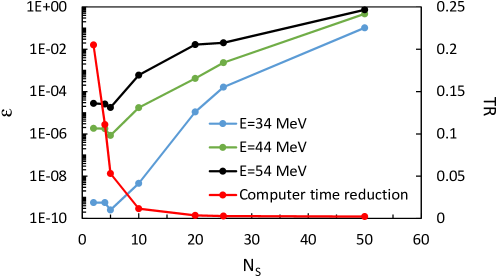
Figure 1: Accuracy (59) (left axis) and computer time reduction (58) (right axis) with the propagation method. The conditions correspond to example 3 ($J=30^{+}$, $a=15$ fm), and the reference calculation is performed with $N_{S}=1,N_{R}=100$ (see text for detail).

Of course, the values presented in Fig. 1 should be considered as indicative only. As the conditions may vary with the energy, the angular momentum, the size of the system, the range of the potential, similar analyses should be performed. However the existence of a compromise, as well as a reasonable lower limit $N_{R}\approx 5$, are common to all conditions of calculations.

7 Conclusion

We propose here an $R$-matrix Fortran package which provides, for a given energy and spin/parity, the collision matrix and the associated wave function. Then the user may easily compute any cross section by using well known formula [25, 26, 7]. Combined with Lagrange functions, the $R$-matrix theory is an efficient tool to determine scattering properties from the coupling potentials. Compared to finite-difference methods, it offers two obvious advantages: $(i)$ non-local potentials are treated on an equal footing, and do not require any specific adaptation; with Lagrange functions, the matrix elements of a local potential are diagonal, whereas they are non-diagonal for non-local potentials. $(ii)$ Closed channels are included consistently with open channels. Possible numerical instabilities, due to the inclusion of closed channels, are absent in the $R$-matrix method.

Single-channel calculations are extremely fast with modern computers. For large-scale calculations (i.e. from several tens of channels), the inversion of the complex matrix $\boldsymbol{C}$ (see eqs. (19)and (39)) is the main numerical issue. We showed that the computer time can be significantly reduced by using the propagation method. For the user, the only change is that the mesh points, where the coupling potentials must be calculated, are different with and without propagation. This technique is therefore simple to implement in any code. In addition, we mentioned that using LAPACK subroutines for the matrix inversion may also speed up the calculation, in particular in a multi-CPU environment using OPENMP.

Solving a coupled-channel system in the continuum is a frequent problem in physics. We believe that this Fortran package is simple to use, as soon as the coupling potentials are determined. These potentials may be deduced from many different models, such as the microscopic RGM method, the CDCC method, standard coupled-channel theories, or many others. Consequently, the present package may be helpful to many potential users who need a minor adaptation of their bound-state codes to extend them to continuum states.

Appendix A

This appendix gives the output of example 1.

total angular momentum= 20
number of basis functions per interval= 60
number of intervals=  1
channel radius=  14.0000
Number of energies:  5
Initial energy:   10.0000
Energy step:   10.0000
E (MeV)=  10.000   Collision matrix=  1.0000E+00  5.9801E-19
E (MeV)=  20.000   Collision matrix=  1.0000E+00  7.4950E-07
E (MeV)=  30.000   Collision matrix=  9.9893E-01  9.0496E-03
E (MeV)=  40.000   Collision matrix=  6.5081E-01  2.9560E-01
E (MeV)=  50.000   Collision matrix=  6.4367E-02  4.1130E-02
Number of energies:  0
Initial energy:    0.0000
Energy step:    0.0000

total angular momentum= 20
number of basis functions per interval= 15
number of intervals=  5
channel radius=  14.0000
Number of energies:  5
Initial energy:   10.0000
Energy step:   10.0000
E (MeV)=  10.000   Collision matrix=  1.0000E+00  5.9631E-19
E (MeV)=  20.000   Collision matrix=  1.0000E+00  7.4950E-07
E (MeV)=  30.000   Collision matrix=  9.9893E-01  9.0496E-03
E (MeV)=  40.000   Collision matrix=  6.5081E-01  2.9560E-01
E (MeV)=  50.000   Collision matrix=  6.4367E-02  4.1130E-02
Number of energies:  0
Initial energy:    0.0000
Energy step:    0.0000

total angular momentum= 20
number of basis functions per interval= 15
number of intervals=  5
channel radius=  16.0000
Number of energies:  5
Initial energy:   10.0000
Energy step:   10.0000
E (MeV)=  10.000   Collision matrix=  1.0000E+00  2.8398E-17
E (MeV)=  20.000   Collision matrix=  1.0000E+00  4.4229E-06
E (MeV)=  30.000   Collision matrix=  9.9879E-01  1.0301E-02
E (MeV)=  40.000   Collision matrix=  6.5059E-01  2.9599E-01
E (MeV)=  50.000   Collision matrix=  6.4381E-02  4.1206E-02
Number of energies:  0
Initial energy:    0.0000
Energy step:    0.0000

In Fig. 2, we show the real part of the wave function at 50 MeV. The internal part (solid line) is computed with Eq. (9), and the external part (dashed line) with Eq. (7). The quality of the matching at the channel radius ($a=16$ fm) supports the accuracy of the calculation. Another test is provided by the stability of the collision matrix against variations of the channel radius and of the basis size.

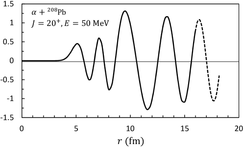
Figure 2: Real part of the $\alpha+^{208}$Pb $J=20^{+}$ wave function at $\mbox{$E_{\mathrm{c}.m.}$}=50$ MeV, with a channel radius $a=16$ fm. The solid and dashed lines represent the internal and external wave functions, respectively.

Appendix B

This appendix gives the output of example 2. The wave function at $\mbox{$E_{\mathrm{c}.m.}$}=36$ MeV is shown in Fig. 3.

total angular momentum=  1
number of basis functions per interval= 60
number of intervals=  1
channel radius=   7.0000
Number of energies:  4
Initial energy:   12.0000
Energy step:   12.0000
E (MeV)= 12.0 phase shift (rad.)=  1.4256E+00 -4.8047E-02 eta_12=  6.7922E-02
E (MeV)= 24.0 phase shift (rad.)=  1.1052E+00 -1.1502E-01 eta_12=  8.2249E-02
E (MeV)= 36.0 phase shift (rad.)=  9.0165E-01 -1.6959E-01 eta_12=  9.9708E-02
E (MeV)= 48.0 phase shift (rad.)=  7.4889E-01 -2.1425E-01 eta_12=  1.1575E-01
Number of energies:  0
Initial energy:    0.0000
Energy step:    0.0000

total angular momentum=  1
number of basis functions per interval= 30
number of intervals=  2
channel radius=   7.0000
Number of energies:  4
Initial energy:   12.0000
Energy step:   12.0000
E (MeV)= 12.0 phase shift (rad.)=  1.4256E+00 -4.8047E-02 eta_12=  6.7922E-02
E (MeV)= 24.0 phase shift (rad.)=  1.1052E+00 -1.1502E-01 eta_12=  8.2249E-02
E (MeV)= 36.0 phase shift (rad.)=  9.0165E-01 -1.6959E-01 eta_12=  9.9708E-02
E (MeV)= 48.0 phase shift (rad.)=  7.4889E-01 -2.1425E-01 eta_12=  1.1575E-01
Number of energies:  0
Initial energy:    0.0000
Energy step:    0.0000

total angular momentum=  1
number of basis functions per interval= 25
number of intervals=  3
channel radius=   8.0000
Number of energies:  4
Initial energy:   12.0000
Energy step:   12.0000
E (MeV)= 12.0 phase shift (rad.)=  1.4258E+00 -4.9358E-02 eta_12=  6.4110E-02
E (MeV)= 24.0 phase shift (rad.)=  1.1052E+00 -1.1506E-01 eta_12=  8.2470E-02
E (MeV)= 36.0 phase shift (rad.)=  9.0182E-01 -1.7002E-01 eta_12=  9.7677E-02
E (MeV)= 48.0 phase shift (rad.)=  7.4900E-01 -2.1469E-01 eta_12=  1.1440E-01
Number of energies:  0
Initial energy:    0.0000
Energy step:    0.0000

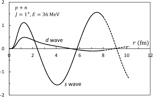
Figure 3: Real part of the $J=1^{+}$ $n-p$ wave function at $\mbox{$E_{\mathrm{c}.m.}$}=36$ MeV, with a channel radius $a=8$ fm (the entrance channel is $L_{\omega}=0$). The solid and dashed lines represent the internal and external wave functions, respectively.

Appendix C

This appendix gives the output of example 3. The wave function at $\mbox{$E_{\mathrm{c}.m.}$}=44$ MeV is presented in Fig. 4.

total angular momentum= 30
number of basis functions per interval= 25
number of intervals=  4
channel radius=  12.0000
Number of energies:  2
Initial energy:   34.0000
Energy step:   10.0000
E (MeV)=  34.000 Amplitude=           9.9408E-01  1.9823E-02  9.9839E-03  6.8090E-03
E (MeV)=  34.000 phase shift (rad.)=  1.3878E-02 -6.5505E-01 -6.6877E-01 -6.7803E-01
E (MeV)=  44.000 Amplitude=           5.3784E-01  1.6169E-01  2.0842E-01  2.1203E-01
E (MeV)=  44.000 phase shift (rad.)=  1.8330E-01  2.4799E-01  3.4390E-02 -7.6706E-02

total angular momentum= 30
number of basis functions per interval= 25
number of intervals=  4
channel radius=  13.0000
Number of energies:  2
Initial energy:   34.0000
Energy step:   10.0000
E (MeV)=  34.000 Amplitude=           9.9373E-01  2.0734E-02  1.0974E-02  7.9570E-03
E (MeV)=  34.000 phase shift (rad.)=  1.4771E-02 -6.5504E-01 -6.6884E-01 -6.7773E-01
E (MeV)=  44.000 Amplitude=           5.3759E-01  1.6176E-01  2.0848E-01  2.1180E-01
E (MeV)=  44.000 phase shift (rad.)=  1.8357E-01  2.4807E-01  3.4413E-02 -7.6101E-02

total angular momentum= 30
number of basis functions per interval= 25
number of intervals=  4
channel radius=  14.0000
Number of energies:  2
Initial energy:   34.0000
Energy step:   10.0000
E (MeV)=  34.000 Amplitude=           9.9370E-01  2.0814E-02  1.1000E-02  7.9145E-03
E (MeV)=  34.000 phase shift (rad.)=  1.4832E-02 -6.5501E-01 -6.6880E-01 -6.7762E-01
E (MeV)=  44.000 Amplitude=           5.3757E-01  1.6177E-01  2.0848E-01  2.1177E-01
E (MeV)=  44.000 phase shift (rad.)=  1.8360E-01  2.4808E-01  3.4417E-02 -7.6024E-02

total angular momentum= 30
number of basis functions per interval= 50
number of intervals=  2
channel radius=  14.0000
Number of energies:  2
Initial energy:   34.0000
Energy step:   10.0000
E (MeV)=  34.000 Amplitude=           9.9370E-01  2.0814E-02  1.1000E-02  7.9145E-03
E (MeV)=  34.000 phase shift (rad.)=  1.4832E-02 -6.5501E-01 -6.6880E-01 -6.7762E-01
 Wave function at a fixed step size
 Channel  1
   2.000 -2.3419E-11 -2.4100E-11
   4.000 -8.4875E-05  9.9903E-05
   6.000  1.3439E-03 -2.6307E-04
   8.000  6.1952E-03  3.7707E-03
  10.000  1.6631E-02 -4.5625E-01
  12.000  5.1200E-02 -3.4580E+00
  14.000 -2.6606E-02  2.1608E+00
  16.000 -3.6187E-02  2.1613E+00
  18.000 -2.4200E-02  1.1868E+00
  20.000 -2.2727E-02  1.0954E+00
 Channel  2
   2.000 -1.5236E-10  2.5608E-10
   4.000  1.6747E-04  2.4738E-05
   6.000 -1.1584E-03  2.4194E-04
   8.000 -5.4272E-03 -7.5530E-03
  10.000 -1.4726E-02  2.4985E-02
  12.000 -3.2496E-02 -1.4804E-02
  14.000  1.2679E-02  2.6010E-02
  16.000  2.6244E-02 -3.9777E-03
  18.000  1.8569E-02 -1.7156E-02
  20.000  1.5656E-02 -1.8832E-02
 Channel  3
   2.000  1.3121E-11  1.2765E-11
   4.000  4.9824E-05 -6.0398E-05
   6.000 -8.3111E-04  8.6104E-05
   8.000 -3.5400E-03 -4.6614E-03
  10.000 -6.1700E-03  1.5577E-02
  12.000 -2.0150E-02  3.4619E-03
  14.000  1.5600E-02  2.2871E-03
  16.000  3.2947E-03 -1.3872E-02
  18.000 -6.5698E-03 -1.1795E-02
  20.000 -8.8601E-03 -9.5665E-03
 Channel  4
   2.000  1.3734E-12 -6.9826E-13
   4.000 -1.4966E-05 -4.1342E-05
   6.000 -9.2885E-04  1.5343E-05
   8.000 -3.5720E-03 -4.1435E-03
  10.000 -4.3643E-03  1.4468E-02
  12.000 -1.3143E-02  1.0031E-02
  14.000  8.5137E-03 -8.1312E-03
  16.000 -8.2890E-03 -6.3665E-03
  18.000 -9.5315E-03  2.3991E-03
  20.000 -7.7940E-03  5.3598E-03
E (MeV)=  44.000 Amplitude=           5.3757E-01  1.6177E-01  2.0848E-01  2.1177E-01
E (MeV)=  44.000 phase shift (rad.)=  1.8360E-01  2.4808E-01  3.4417E-02 -7.6024E-02
 Wave function at a fixed step size
 Channel  1
   2.000  5.1169E-10  2.2624E-09
   4.000  3.5023E-03 -1.8169E-03
   6.000 -1.5940E-02  3.4657E-02
   8.000 -4.2896E-03 -1.2585E-02
  10.000  3.9204E-01 -2.5708E+00
  12.000  6.1462E-01  9.4364E-02
  14.000  4.8419E-01  4.5397E-01
  16.000  6.2567E-01 -7.3889E-01
  18.000  2.6037E-01 -1.7221E+00
  20.000 -5.4054E-01  1.0385E-01
 Channel  2
   2.000  5.8255E-08 -8.2729E-09
   4.000 -9.1816E-03 -9.0830E-03
   6.000  5.6940E-02 -4.5175E-02
   8.000  4.0620E-01  1.4412E-02
  10.000  1.7297E-01 -2.1291E-01
  12.000 -1.5159E-01 -1.5453E-01
  14.000 -1.6344E-01 -1.1417E-01
  16.000 -6.0469E-02 -1.8073E-01
  18.000  1.3399E-01 -1.2785E-01
  20.000  1.3510E-01  1.2128E-01
 Channel  3
   2.000  1.2179E-09 -2.8657E-09
   4.000 -5.7318E-03 -1.0215E-03
   6.000  3.8482E-02 -6.1791E-03
   8.000  1.8361E-01 -1.8840E-01
  10.000 -1.1708E-01 -3.7177E-01
  12.000 -2.2134E-01  1.8160E-01
  14.000 -1.1709E-01  2.3285E-01
  16.000 -2.0146E-01  1.4434E-01
  18.000 -2.2135E-01 -9.3229E-02
  20.000  5.5096E-02 -2.2853E-01
 Channel  4
   2.000 -7.7840E-11 -2.7581E-10
   4.000 -3.8399E-03  9.1628E-04
   6.000  3.0656E-02  2.6539E-02
   8.000  1.3643E-01 -3.1429E-01
  10.000 -3.8360E-01 -2.3309E-01
  12.000  9.9274E-02  2.8378E-01
  14.000  2.2823E-01  1.4253E-01
  16.000  1.6361E-01  1.9467E-01
  18.000 -4.8941E-02  2.4076E-01
  20.000 -2.3968E-01  1.2736E-02

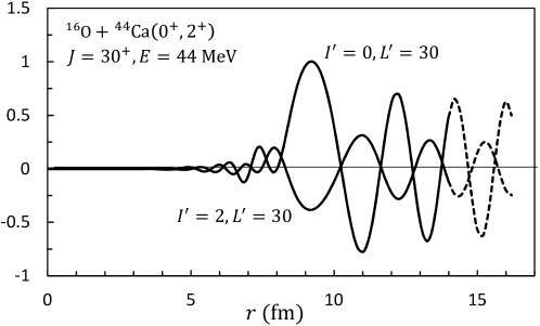
Figure 4: Real part of the $J=30^{+}$ ${}^{16}{\mathrm{O}}+^{44}$Ca wave function at $\mbox{$E_{\mathrm{c}.m.}$}=44$ MeV, with a channel radius $a=14$ fm. We show the elastic ($I^{\prime}=0,L^{\prime}=30$) and inelastic ($I^{\prime}=2,L^{\prime}=30$) components. The solid and dashed lines represent the internal and external wave functions, respectively.

Appendix D

This appendix gives the output of example 4. The wave function at $\mbox{$E_{\mathrm{c}.m.}$}=4$ MeV is presented in Fig. 5.

total angular momentum=  3
number of basis functions per interval= 25
number of intervals=  4
channel radius=   9.0000
Number of energies:  5
Initial energy:    4.0000
Energy step:    4.0000
E (MeV)=   4.000 Amplitude=           6.3596E-01
E (MeV)=   4.000 phase shift (rad.)= -9.4942E-02
E (MeV)=   8.000 Amplitude=           1.7408E-01  4.1658E-02  5.2298E-02  2.6680E-02
E (MeV)=   8.000 phase shift (rad.)= -1.0478E+00 -3.6134E-01 -9.3976E-02 -3.3158E-01
E (MeV)=  12.000 Amplitude=           7.7759E-02  3.8135E-02  3.0539E-02  7.3661E-02
E (MeV)=  12.000 phase shift (rad.)=  1.1344E+00  1.2203E+00 -8.6494E-01 -5.5400E-01
E (MeV)=  16.000 Amplitude=           4.2879E-02  2.7207E-02  2.9671E-02  3.4527E-02
                                      2.9332E-03  1.0489E-03  1.8585E-04  2.5162E-05
E (MeV)=  16.000 phase shift (rad.)=  3.3080E-01  4.2471E-01  1.2639E+00 -1.2662E+00
                                     -6.6359E-01 -9.7805E-01 -1.3598E+00  1.5139E+00
E (MeV)=  20.000 Amplitude=           2.8051E-02  1.9170E-02  1.9106E-02  2.0175E-02
                                      4.7665E-03  6.3974E-03  9.4889E-03  5.8624E-03
E (MeV)=  20.000 phase shift (rad.)= -4.1339E-01 -5.1731E-01  4.2013E-01  1.0489E+00
                                      7.7182E-01  1.3264E+00  1.4657E+00  1.2864E+00

Number of energies:  0
Initial energy:    0.0000
Energy step:    0.0000

total angular momentum=  3
number of basis functions per interval= 25
number of intervals=  4
channel radius=  10.0000
Number of energies:  5
Initial energy:    4.0000
Energy step:    4.0000
E (MeV)=   4.000 Amplitude=           6.3211E-01
E (MeV)=   4.000 phase shift (rad.)= -1.0498E-01
E (MeV)=   8.000 Amplitude=           1.8026E-01  4.3834E-02  5.2228E-02  2.7052E-02
E (MeV)=   8.000 phase shift (rad.)= -1.0365E+00 -3.7119E-02 -1.2120E-01 -3.7472E-01
E (MeV)=  12.000 Amplitude=           8.3944E-02  1.3480E-02  4.0382E-02  8.1238E-02
E (MeV)=  12.000 phase shift (rad.)=  1.1559E+00 -1.5076E+00 -8.3169E-01 -6.3383E-01
E (MeV)=  16.000 Amplitude=           4.3161E-02  2.7045E-02  2.9524E-02  3.4464E-02
                                      2.9445E-03  1.0500E-03  1.8528E-04  2.5063E-05
E (MeV)=  16.000 phase shift (rad.)=  3.3205E-01  4.2416E-01  1.2627E+00 -1.2686E+00
                                     -6.5988E-01 -9.7391E-01 -1.3555E+00  1.5185E+00
E (MeV)=  20.000 Amplitude=           2.8039E-02  1.9165E-02  1.9073E-02  2.0003E-02
                                      4.7594E-03  6.3858E-03  9.4702E-03  5.8594E-03
E (MeV)=  20.000 phase shift (rad.)= -4.1803E-01 -5.1340E-01  4.2415E-01  1.0520E+00
                                      7.7283E-01  1.3272E+00  1.4670E+00  1.2879E+00

Number of energies:  0
Initial energy:    0.0000
Energy step:    0.0000

total angular momentum=  3
number of basis functions per interval= 20
number of intervals=  4
channel radius=  11.0000
Number of energies:  5
Initial energy:    4.0000
Energy step:    4.0000
E (MeV)=   4.000 Amplitude=           6.1525E-01
E (MeV)=   4.000 phase shift (rad.)= -1.0040E-01
E (MeV)=   8.000 Amplitude=           1.8113E-01  6.6769E-02  4.8913E-02  2.4643E-02
E (MeV)=   8.000 phase shift (rad.)= -1.0734E+00 -1.5641E-01 -1.0245E-01 -4.0518E-01
E (MeV)=  12.000 Amplitude=           8.7310E-02  4.2829E-02  4.0388E-02  7.3597E-02
E (MeV)=  12.000 phase shift (rad.)=  1.0617E+00 -1.4261E+00 -9.3782E-01 -7.2888E-01
E (MeV)=  16.000 Amplitude=           4.3124E-02  2.7057E-02  2.9530E-02  3.4450E-02
                                      2.9433E-03  1.0489E-03  1.8491E-04  2.4997E-05
E (MeV)=  16.000 phase shift (rad.)=  3.3174E-01  4.2457E-01  1.2632E+00 -1.2680E+00
                                     -6.5924E-01 -9.7341E-01 -1.3553E+00  1.5188E+00
E (MeV)=  20.000 Amplitude=           2.8037E-02  1.9167E-02  1.9080E-02  2.0027E-02
                                      4.7582E-03  6.3842E-03  9.4671E-03  5.8584E-03
E (MeV)=  20.000 phase shift (rad.)= -4.1741E-01 -5.1378E-01  4.2378E-01  1.0520E+00
                                      7.7293E-01  1.3273E+00  1.4670E+00  1.2880E+00

Number of energies:  0
Initial energy:    0.0000
Energy step:    0.0000

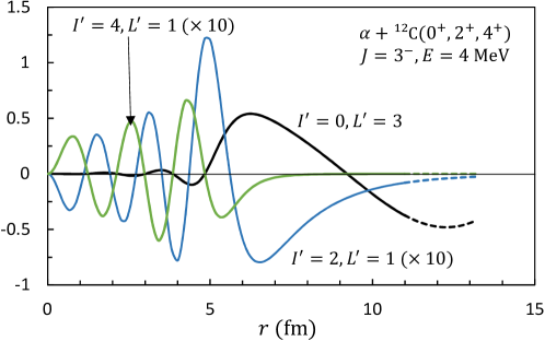
Figure 5: Real part of the $J=3^{-}$ $\alpha+^{12}$C wave function at $\mbox{$E_{\mathrm{c}.m.}$}=4$ MeV, with a channel radius $a=11$ fm. We show the elastic ($I^{\prime}=0,L^{\prime}=3$) and two inelastic components ($I^{\prime}=2,L^{\prime}=1$ and $I^{\prime}=4,L^{\prime}=1$). The solid and dashed lines represent the internal and external wave functions, respectively.

Appendix E

This appendix gives the output of example 5. The wave functions at $\mbox{$E_{\mathrm{c}.m.}$}=0.1$ and 10 MeV are presented in Fig. 6.

total angular momentum=  0
number of basis functions per interval= 10
number of intervals=  1
channel radius=   8.0000
Number of energies:  2
Initial energy:    0.1000
Energy step:    9.9000
E (MeV)=   0.100 phase shift (deg.)= -1.5077E+01  1.0000E+00
E (MeV)=  10.000 phase shift (deg.)=  8.5637E+01  1.0000E+00
Number of energies:  0
Initial energy:    0.0000
Energy step:    0.0000

total angular momentum=  0
number of basis functions per interval= 15
number of intervals=  1
channel radius=   8.0000
Number of energies:  2
Initial energy:    0.1000
Energy step:    9.9000
E (MeV)=   0.100 phase shift (deg.)= -1.5077E+01  1.0000E+00
E (MeV)=  10.000 phase shift (deg.)=  8.5637E+01  1.0000E+00
Number of energies:  0
Initial energy:    0.0000
Energy step:    0.0000

total angular momentum=  0
number of basis functions per interval= 15
number of intervals=  1
channel radius=  12.0000
Number of energies:  2
Initial energy:    0.1000
Energy step:    9.9000
E (MeV)=   0.100 phase shift (deg.)= -1.5079E+01  1.0000E+00
E (MeV)=  10.000 phase shift (deg.)=  8.5635E+01  1.0000E+00
Number of energies:  0
Initial energy:    0.0000
Energy step:    0.0000
 

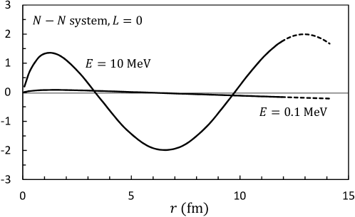
Figure 6: Real part of the $L=0$ nucleon-nucleon wave function with the non-local potential (57) at two energies: $\mbox{$E_{\mathrm{c}.m.}$}=0.1$ and 10 MeV. The channel radius is $a=12$ fm. The solid and dashed lines represent the internal and external wave functions, respectively.

References

- [1] T. Tamura, Rev. Mod. Phys. 37 (1965) 679.
- [2] G. R. Satchler, Direct Nuclear Reactions, Oxford (1983).
- [3] I. J. Thompson, Comput. Phys. Rep. 7 (1988) 167.
- [4] L. A. Morgan, J. Tennyson, C. J. Gillan, Comput. Phys. Commun. 114 (1998) 120.
- [5] M. Plummer, C. J. Noble, J. Phys. B 32 (14) (1999) L345.
- [6] P. Burke, R-Matrix Theory of Atomic Collisions. Application to Atomic, Molecular and Optical Processes, Vol. 61 of Springer Series on Atomic, Optical, and Plasma Physics, Springer, 2011.
- [7] L. F. Canto, M. S. Hussein, Scattering Theory of Molecules, Atoms and Nuclei, World Scientific Publishing, Singapore, 2013.
- [8] M. V. Zhukov, B. V. Danilin, D. V. Fedorov, J. M. Bang, I. J. Thompson, J. S. Vaagen, Phys. Rep. 231 (1993) 151.
- [9] I. J. Thompson, F. M. Nunes, B. V. Danilin, Comput. Phys. Commun. 161 (2004) 87.
- [10] H. Horiuchi, Prog. Theor. Phys. Suppl. 62 (1977) 90.
- [11] M. Theeten, H. Matsumura, M. Orabi, D. Baye, P. Descouvemont, Y. Fujiwara, Y. Suzuki, Phys. Rev. C 76 (2007) 054003.
- [12] S. Quaglioni, P. Navrátil, Phys. Rev. Lett. 101 (2008) 092501.
- [13] H. Kamada, A. Nogga, W. Glöckle, E. Hiyama, M. Kamimura, K. Varga, Y. Suzuki, M. Viviani, A. Kievsky, S. Rosati, J. Carlson, Steven C. Pieper, R. B. Wiringa, P. Navrátil, B. R. Barrett, N. Barnea, W. Leidemann, G. Orlandini, Phys. Rev. C 64 (2001) 044001
- [14] E. Hiyama, Y. Kino, M. Kamimura, Prog. Part. Nucl. Phys. 51 (2003) 223.
- [15] M. Viviani, A. Kievsky, S. Rosati, Phys. Rev. C 71 (2005) 024006.
- [16] J. Mitroy, S. Bubin, W. Horiuchi, Y. Suzuki, L. Adamowicz, W. Cencek, K. Szalewicz, J. Komasa, D. Blume, K. Varga, Rev. Mod. Phys. 85 (2013) 693.
- [17] K. Varga, Y. Suzuki, Phys. Rev. C 52 (1995) 2885.
- [18] J. Raynal, in ”Computing as a Language of Physics”, Trieste 1971, IAEA, Vienna (1972) p. 281.
- [19] W. Baylis, S. Peel, Comput. Phys. Commun. 25 (1982) 7.
- [20] A. E. Thorlacius, E. D. Cooper, J. Comput. Phys. 72 (1987) 70.
- [21] E. P. Wigner, Phys. Rev. 70 (1946) 606.
- [22] I. J. Thompson, B. V. Danilin, V. D. Efros, J. S. Vaagen, J. M. Bang, M. V. Zhukov, Phys. Rev. C 61 (2000) 024318.
- [23] P. Descouvemont, E. M. Tursunov, D. Baye, Nucl. Phys. A 765 (2006) 370.
- [24] D. Baye, P. Capel, P. Descouvemont, Y. Suzuki, Phys. Rev. C 79 (2009) 024607.
- [25] A. M. Lane, R. G. Thomas, Rev. Mod. Phys. 30 (1958) 257.
- [26] P. Descouvemont, D. Baye, Rep. Prog. Phys. 73 (2010) 036301.
- [27] D. Baye, Phys. Rep. 565 (2015) 1.
- [28] M. Hesse, J. M. Sparenberg, F. Van Raemdonck, D. Baye, Nucl. Phys. A 640 (1998) 37.
- [29] M. Hesse, J. Roland, D. Baye, Nucl. Phys. A 709 (2002) 184.
- [30] K. L. Baluja, P. G. Burke, L. A. Morgan, Comput. Phys. Commun. 27 (1982) 299.
- [31] L. A. Morgan, Comput. Phys. Commun. 31 (1984) 419.
- [32] F. C. Barker, H. J. Hay, P. B. Treacy, Aust. J. Phys. 21 (1968) 239.
- [33] I. J. Thompson, NIST Handbook of Mathematical Functions, Cambridge University Press, 2010, p. 741.
- [34] A. B. Olde Daalhuis, NIST Handbook of Mathematical Functions, Cambridge University Press, 2010, p. 321.
- [35] C. Bloch, Nucl. Phys. 4 (1957) 503.
- [36] R. F. Barrett, B. A. Robson, W. Tobocman, Rev. Mod. Phys. 55 (1983) 155.
- [37] P. J. A. Buttle, Phys. Rev. 160 (1967) 719.
- [38] J. C. Light, R. B. Walker, J. Chem. Phys. 65 (1976) 4272.
- [39] D. Baye, P. Descouvemont, Nucl. Phys. A 407 (1983) 77.
- [40] D. Baye, M. Hesse, J.-M. Sparenberg, M. Vincke, J. Phys. B 31 (1998) 3439.
- [41] T. Druet, D. Baye, P. Descouvemont, J.-M. Sparenberg, Nucl. Phys. A 845 (2010) 88.
- [42] D. Baye, J. Goldbeter, J.-M. Sparenberg, Phys. Rev. A 65 (2002) 052710.
- [43] D. Baye, M. Hesse, M. Vincke, Phys. Rev. E 65 (2002) 026701.
- [44] V. Szalay, T. Szidarovszky, G. Czakó, A. G. Császár, Journal of Mathematical Chemistry 50 (2011) 636.
- [45] T. Druet, P. Descouvemont, Eur. Phys. J. A 48 (2012) 147.
- [46] M. Rhoades-Brown, M. H. Macfarlane, S. C. Pieper, Phys. Rev. C 21 (1980) 2417.
- [47] Lapack library, http://www.netlib.org/lapack.
- [48] M. Abramowitz, I. A. Stegun, Handbook of Mathematical Functions, Dover, London, 1972.
- [49] S. Zhang, J. M. Jin, Computation of Special Functions, Wiley-Interscience, 1996, source available at http://jin.ece.illinois.edu/routines/routines.html.
- [50] A. Barnett, Comput. Phys. Commun. 35 (1984) C812.
- [51] W. H. Press, B. P. Flannery, S. A. Teukolsky, W. T. Vettering, Numerical Recipes, Cambridge University Press (1986).
- [52] G. Goldring, M. Samuel, B. A. Watson, M. C. Bertin, S. L. Tabor, Phys. Lett. B 32 (1970) 465.
- [53] R. V. Reid, Ann. Phys. 50 (1968) 411.
- [54] M. Rhoades-Brown, M. H. Macfarlane, S. C. Pieper, Phys. Rev. C 21 (1980) 2436.
- [55] S. Raman, C. W. Nestor, P. Tikkanen, At. Data Nucl. Data Tables 78 (2001) 1.
- [56] Y. Yamaguchi, Phys. Rev. 95 (1954) 1628.